Article

Visibility Prediction over South Korea Based on Random Forest

Convergence Meteorological Research Department, National Institute of Meteorological Sciences, Seogwipo, Jeju 63569, Korea
*
Author to whom correspondence should be addressed.
Atmosphere 2021, 12(5), 552; https://doi.org/10.3390/atmos12050552
Submission received: 22 March 2021 / Revised: 7 April 2021 / Accepted: 23 April 2021 / Published: 25 April 2021
(This article belongs to the Section Air Quality)

Abstract

:
In this study, the visibility of South Korea was predicted (VISRF) using a random forest (RF) model based on ground observation data from the Automated Synoptic Observing System (ASOS) and air pollutant data from the European Centre for Medium-Range Weather Forecasts (ECMWF) Copernicus Atmosphere Monitoring Service (CAMS) model. Visibility was predicted and evaluated using a training set for the period 2017–2018 and a test set for 2019. VISRF results were compared and analyzed using visibility data from the ASOS (VISASOS) and the Unified Model (UM) Local Data Assimilation and Prediction System (LDAPS) (VISLDAPS) operated by the Korea Meteorological Administration (KMA). Bias, root mean square error (RMSE), and correlation coefficients (R) for the VISASOS and VISLDAPS datasets were 3.67 km, 6.12 km, and 0.36, respectively, compared to 0.14 km, 2.84 km, and 0.81, respectively, for the VISASOS and VISRF datasets. Based on these comparisons, the applied RF model offers significantly better predictive performance and more accurate visibility data (VISRF) than the currently available VISLDAPS outputs. This modeling approach can be implemented by authorities to accurately estimate visibility and thereby reduce accidents, risks to public health, and economic losses, as well as inform on urban development policies and environmental regulations.

1. Introduction

Visibility refers to the maximum horizontal distance visible to the human eye as a measure of the distance through which an object or light can be identified. The World Meteorological Organization (WMO) [1] defines the meteorological optical range (MOR) as the distance at which light intensity decreases to 5% of its original level [2]. This provides a useful metric of visibility based on distinguishing and measuring objects, such as buildings, identified by human observation or by detecting the amount of attenuated or scattered light using optical sensors [3]. Visibility is often measured using networks of visibility sensors, such as Vaisala or Biral sensors, and can reach 300 km when only Rayleigh scattering and gas absorption are taken into account [4]; however, distances of 145–225 km are typical for unpolluted atmospheric conditions, and distances of 10–100 km are commonly recorded [5]. Importantly, precipitation and air pollution can have significant impacts on visibility, with low-visibility conditions of a few kilometers not uncommon [6], and such effects have impacts on weather and climate change [7,8]. In addition, low visibility is linked to socioeconomic losses, including road and air traffic accidents and public health risks [9,10,11].
Visibility is generally predicted spatiotemporally using numerical weather prediction (NWP) models such as the Unified Model (UM) and the Weather Research and Forecasting (WRF) model [12,13]. NWP models predict visibility based on various meteorological variables including the liquid/ice water content of clouds and water droplets, aerosol concentrations, and rain/snow, which are included in the parameterization of cloud physics and microphysical processes [14,15,16]. However, because visibility is sensitive to a range of variables, prediction based on NWP is challenging, yielding poor predictive performance compared to other meteorological variables such as precipitation [3,10,12,17,18,19]. Therefore, various studies have been reported that focus on parameterization improvement [14,20,21], data assimilation [3], and ensemble construction [19]. Nevertheless, the low predictive accuracy of NWP models and their high computational requirements remain significant disadvantages [22]. As an alternative approach, machine learning and regression analysis based on the relationship between visibility and various meteorological variables (derived from ground-based observations and model prediction data) are increasingly being applied [13,16].
The generation and release of anthropogenic and natural air pollutants reduce visibility [23,24,25,26,27] and have significant impacts on visibility prediction [28,29,30,31]. Therefore, relational equations for predicting visibility are often derived using meteorological data, such as relative humidity, pollution concentrations, and precipitation [30,32,33,34,35,36]. However, low correlation coefficients have been derived between these variables and visibility (typically between −0.2 and −0.5), which limits the predictive power of models based on linear and nonlinear correlations [26]. To overcome this, visibility prediction using machine learning methods including artificial neural networks (ANNs), support vector machines (SVMs), and extreme learning machines (ELMs) is being increasingly explored (e.g., [16,19,22,37]). In particular, machine learning offers high utility and performance for estimating visibility based on the complex relationships between visibility and meteorological datasets [38].
In this study, a machine-learning-based prediction model is constructed and evaluated for the visibility prediction for the specific purposes of improving the speed and accuracy of existing visibility data predicted by the NWP model in South Korea. Specifically, meteorological observations and air pollutant data are used as input data of a random forest (RF) model. Among the numerous supervised machine learning methods, a decision tree (DT) can exclude many variables from the prediction model construction by pruning [39]; and the k-nearest neighbor (k-NN) is highly dependent on the number of clusters k in the data [40]. Regarding the support vector machine (SVM), there is a difference in prediction performance depending on the settings such as kernel and cost [41]. Deep learning methods such as ANN and ELM exhibit varying predictive performances depending on the number of hidden single- or multi-layers and weights for each variable; the learning and prediction speeds of deep learning methods are slower than other machine learning methods [42]. Therefore, its prediction performance is more dependent on the setting method for model construction than the feature of the input data. In contrast, the prediction algorithm of the RF model ensembles the results of numerous decision trees combined according to a random method based on the input data; thus, the prediction variability is not large [43,44]. Additionally, the RF approach also prevents overfitting of the model and produces optimal results by rapidly processing significant amounts of data [45,46]. The remainder of the paper is organized as follows: the meteorological input data, RF model, and predictive performance of the model are described in Section 2; Section 3 evaluates the model outputs in comparison with observation data and NWP model outputs; and finally, Section 4 presents the main conclusions of the study.

2. Data and Research Methods

2.1. Datasets

In this study, ground-based observation data from the Automated Synoptic Observing System (ASOS) and air pollutant data from the European Center for Medium-Range Weather Forecasts (ECMWF) Copernicus Atmosphere Monitoring Service (CAMS) [47,48] were collected from 1 January 2017, to 31 December 2019. ASOS records a range of meteorological information including temperature, relative humidity (RH), pressure, precipitation, and visibility at each site every minute (Table 1). Air pollutant data of the CAMS model generate +3–120-h prediction data at 3-h intervals at 0000 UTC and 1200 UTC twice a day from 2017, and provide data with a spatial resolution of 0.125° × 0.125°. Here, +3-h, +6-h, +9-h, and +12-h datasets predicted for each running time of 0000 UTC and 1200 UTC were used. Based on the location information of the sites shown in Table 1, spatially linear interpolated CAMS air pollutants data were derived at 3-h intervals.
The air pollutant datasets included particulate matter (sea salt (SS), dust (DU), organic matter (OM), black carbon (BC), and sulfate (SU)) [11,22] as well as ozone (O3), nitrogen dioxide (NO2), sulfur dioxide (SO2), and carbon monoxide (CO), all of which affect visibility [7,32,49,50]. These are the only model prediction datasets offering global-scale air pollutant information, including the Modern-Era Retrospective Analysis for Research and Applications version 2 (MERRA-2) [51,52], with a correlation coefficient in the range 0.5–0.8 and uncertainty in the range 10–20% compared to ground observations [53,54,55]. However, MERRA-2 has a temporal resolution of 1-h and a relatively low spatial resolution (0.5° × 0.625°), which is unsuitable for local-scale analyses; discrepancies with ground-based measurements can, therefore, be larger for MERRA-2 data than with CAMS model outputs [55]. Furthermore, as the CAMS model provides air pollutant data as mass mixing ratios (kg/kg), these data were converted to mass concentrations (μg/m3) using Equation (1) for the RF model input. The CAMS mass mixing ratios (MMRs) were assumed to be similar to those in the lower atmosphere, and the ground-level mass concentrations were calculated using the ASOS temperature and pressure observations [47,56].
M a s s   c o n c . = M M R × P R T
where P and T are the pressure (Pa) and temperature (K) derived from the ASOS, respectively, and R is the specific gas constant (287.06 J/(kg·K)).

2.2. Evaluation of Predictions

To evaluate the accuracy of the visibility predictions, variability data from the ASOS and the UM Local Data Assimilation and Prediction System (LDAPS) [57] were used. As shown in Figure 1, the ASOS visibility data were acquired using the Biral VPF730 (24 sites) and Vaisala PWD22 (48 sites) models based on 72 observation sites distributed across South Korea (Table 1). These sensors measure visibility in the range 0.01–20 km with uncertainty of ±10–15% within the measurement range [58,59]. The red and blue points in Figure 1 indicate the representative sites in urban and island regions analyzed in the results (Section 3). Visibility data from the UM LDAPS are local predictions provided by the Korea Meteorological Administration (KMA) with a spatiotemporal resolution of 1.5 × 1.5 km2 at 3-h intervals eight times a day (+0–36-h predictions at 3-h intervals at 0000, 0600, 1200, and 1800 UTC and +0-h and 3-h predictions at 0300, 0900, 1500, and 2100 UTC), derived using a 3-dimensional variational data assimilation (3DVAR) method [60,61]. We used the analysis fields data (+0-h), which predicts at 3-h intervals eight times a day. As the UM LDAPS predicts visibility in the range 0.01–100 km, data for ranges > 20 km were limited to 20 km (maximum), according to the measurement range of visibility sensors, and analyzed. The same conditions were applied to results predicted by using the RF model. For comparison, bias, root mean square error (RMSE), and correlation coefficients (R) were calculated for the visibility data predicted by the RF (VISRF) and LDAPS (VISLDAPS) models, and the visibility measurements from the ASOS (VISASOS), using Equations (2–4):
b i a s = i = 1 N ( P i M i ) / N
R M S E = i = 1 N ( P i M i ) 2 / N
R = i = 1 N ( P i P ¯ ) ( M i M ¯ ) / i = 1 N ( P i P ¯ ) 2 i = 1 N ( M i M ¯ ) 2
where P is the prediction, M is the measurement, and N is the number of data.

2.3. Random Forest (RF) Model Sets

The random forest adopted in this study constructs N decision trees by combining variables randomly selected from each node to grow a regression tree, as shown in Figure 2. Further, the results of individual decision trees are ensembled to obtain the prediction result [43,44]. Thus, in the RF ensemble learning method, each tree contributes to the final prediction [62]. RF ensembles the results of all decision trees to obtain a large prediction variability and avoid overfitting, producing optimal results. The adopted RF method ensembles the results of a decision tree to optimize results by minimizing prediction variability and overfitting, being widely applied given its high prediction accuracy and ability to rapidly process large datasets [45]. The ‘Ranger’ R package was used to construct the RF model, which shows similar prediction performance and ten-times faster learning and prediction speeds than other RF packages [46].
The data, at 3-h intervals for 72 ASOS sites shown in Table 1, were used as training and test datasets in the RF model. The training set was composed of data from 1 January 2017, to 31 December 2018, and the test set was composed of data from 1 January 2019, to 31 December 2019. As hygroscopic aerosols and pollutants show deliquescent properties in wet and high RH conditions [31], visibility predictions are often limited to days with no precipitation and RH < 80% [9,25,26,28]. Here, to predict visibility under various weather conditions, a visibility prediction model was constructed using a learning training set for all the variables shown in Table 1, thus removing the restriction of meteorological conditions. At this time, mtry was set to 4, which is sqrt (number of variables) (default), and the tree was set to 500 (default). As the number of trees increased in the RF model, more trees were averaged, thereby reducing overfitting to construct a more stable prediction model. However, even with more than 500 trees, no significant change in the out-of-bag (OOB) estimation result was observed, with only the training time increasing [63].
Figure 3 shows the permutation importance of the input variables input in the RF model. RH has a well-known influence on visibility, and among the air pollutants, SU and CO have high importance [28,30,64,65]. In addition to the meteorological variables, time and location variables also influence visibility predictions. In comparison, wind direction (WD) had the lowest influence on visibility predictions (0.23) among the input meteorological variables. When this variable was removed from the RF model, the OOB error (RMSE) was 2.46 km and R was 0.85.
Figure 4 shows the RF results using training data (2017–2018). The RF model predicts variables in the direction of lowering the variance but shows a positive bias for low predicted values and a negative bias for relatively high values [66,67]. Therefore, bias correction was performed using the equation Y = 1.18 × −2.49, which increased the predictive performance of the model relative to the VISASOS data, with an RMSE of 1.04 km (without bias correction) and 0.88 km (with bias correction).

3. Results and Discussion

Figure 5 shows VISASOS, VISLDAPS, and VISRF from 1 January to 31 December 2019, as a time-series scatter plot. Based on Figure 5a, the frequency of VISLDAPS data exceeding 20 km was high (approximately 63% of the entire dataset) irrespective of VISASOS. This indicates that the LDAPS tended to over-predict visibility compared to the observational data. During this period, VISLDAPS predictions showed large differences relative to VISASOS, with an overall bias of 3.67 km, an RMSE of 6.12 km, and an R of 0.35; these results indicate low predictive performance. In comparison, VISRF, predicted using the RF model (Figure 5b), was relatively consistent with the 1:1 line with VISASOS, with a bias of 0.14 km, an RMSE of 2.84 km, and an R of 0.81. Figure 5c shows the time-series of the daily mean VISASOS, VISLDAPS, and VISRF for all of the observation sites. VISLDAPS predicted values (following the same method currently employed by the KMA) were high due relative to VISASOS observations due to the large number of cases exceeding 20 km (mean = 17.98 km), with a bias of 3.61 km, an RMSE of 4.53 km, and an R of 0.71. Comparatively, the RF-derived VISRF estimates show better predictive performance, with a bias of 0.12 km, an RMSE of 1.54 km, and a high R of 0.89.
Table 2 shows monthly comparisons of VISASOS, VISLDAPS, and VISRF alongside monthly mean data for the meteorological variables used in the RF model. The Korean Peninsula experiences a rainy season from late spring to late autumn (April–October), and in summer (June–August), the temperature and RH are high, with many cloudy days due to general low-pressure conditions [68,69,70]; meteorological conditions have the opposite characteristics during the winter season (September–February). Therefore, during the rainy season, with the exceptions of SS, DU, and O3, which naturally occur due to higher RH and rainfall, the mass concentrations of anthropogenic air pollutants tend to decrease [34,71]. SS and O3 generally have high mass concentrations on islands and near coastal areas, increasing in association with precipitation, surface temperature, and wind speed during the rainy season [72]. In the case of DU, mass concentrations are via inward transport from surrounding dry areas, such as large cities and deserts, during spring and winter when high pressure and sunny conditions dominate [26,73,74]. In contrast, during the winter and spring dry season (November–March), OM, BC, SU, NO2, SO2, and CO tend to increase as a result of fossil fuel burning for heating [53,75,76,77]. Based on the CAMS model data analyses, these air pollutants showed strong positive correlations (R = 0.53–0.98); the VISASOS data are strongly affected by RH, precipitation, and air pollutants, although these effects vary seasonally. Overall, VISASOS was negatively correlated with RH, precipitation, and air pollutants, with mean R-values of −0.57, −0.25, and −0.20 during the rainy season, and −0.59, −0.16, and −0.48 during the dry season, respectively.
The VISLDAPS predictions in Table 2 were approximately 3 km higher than the VISASOS observations, with a mean RMSE of 5 km or more and R-values ranging from as low as 0.11 to 0.54. The VISLDAPS model tended to overestimate visibility under clear conditions and showed poor predictive performance on a monthly timescale. In contrast, the VISRF predictions had a bias of just −0.22 km, an RMSE of 3.01 km, and an R of 0.75 during the rainy season, compared with a bias of 0.63 km, an RMSE of 2.56 km, and an R of 0.87 during the dry season. These results indicate that the predictive performance of the RF model is best during the dry season, when RH and precipitation are high and the mass concentrations of air pollutants are low [29,31]. For example, in September, when RH was as high as 81.96%, precipitation was 1.00 mm (approximately 10 precipitation days), and the mass concentrations of air pollutants were relatively low, the VISRF predictions had a bias of 0.17 km, an RMSE of 3.26 km, and an R of 0.71, corresponding to the poorest predictive performance. By comparison, in January, when the RH was as low as 54.66%, precipitation was 0.16 mm (approximately 3 precipitation days), and the mass concentrations of air pollutants were relatively high, the VISRF predictions had a bias of 0.61 km, an RMSE of 2.23 km, and an R of 0.91, corresponding to the best predictive performance.
For further comparison, Figure 6 shows daily mean VISASOS, VISLDAPS, and VISRF for each of the five ASOS sites representing urban and island regions. The urban region has populations exceeding 1 million and are located away from the coast, namely Seoul (#108), Suwon (#119), Cheongju (#131), Daegu (#143), and Gwangju (#156); the island region has populations less than 500,000, namely Ulleungdo (#115), Heuksando (#169), Gosan (#185), Seongsan (#188), and Jindogun (#268). Notably, the urban region experienced similar temperatures to the island region due to urban heat island effects but experienced fewer precipitation days, lower wind speeds, and higher concentrations of air pollutants [8,22,78].
In the selected urban region (Figure 6a and Table 3), RH was 9.53% lower than the island region during the study period, precipitation was 0.26 mm lower, and 22 fewer precipitation days occurred, whereas the mass concentrations of air pollutants were between 33% (SU) and 1150% (NO2) higher. In particular, for Seoul (#108) in the urban region, with a population of close to 10 million, the mass concentrations of air pollutants were between 141% (DU) and 4435% (NO2) higher than Ulleungdo (#115) in the island region, indicating the cleanest air quality (OM: 530%, BC: 700%, SU: 208%, SO2: 2243%, CO: 379%). The correlations (R) between RH and precipitation and anthropogenic air pollutants in the VISRF predictions for the urban region ranged from −0.52 (SO2) to −0.72 (SU) (Table 4), and similar relationships were observed between the VISASOS observations and these meteorological variables. SU is known to strongly attenuate visibility, worsening visibility relative to other pollutants including OM, BC, and CO [32,50,65]. In particular, as the mass concentrations of air pollutants are highest during the dry season, visibility in the urban region was greatly reduced compared to the island region during this season (mean visibility was 0.72 km lower; Figure 6c). During the dry season, VISRF predictions for the urban region had a bias of −0.26 km, an RMSE of 2.10 km, and an R of 0.85.
In comparison, in the selected island region (Figure 6b), the correlations between RH and precipitation and air pollutant concentrations in the VISRF model were higher than in the urban region (R = −0.72 and −0.41, respectively) (Table 4). Therefore, in the island region, VISASOS was low during the rainy season when precipitation was high (Figure 6d), and the VISRF predictions were very similar to the observations, with a bias of 0.01 km, an RMSE of 1.74 km, and an R of 0.89. In contrast, the VISLDAPS model results over-predicted visibility in the island region, where the mass concentrations of air pollutants were low, with a bias of 4.23 km, an RMSE of 5.45 km, and an R of 0.40. Thus, the results of the visibility prediction of UM LDAPS were %bias and %RMSE of 27.84% and 35.88%, respectively, compared to the mean visibility; these results indicate a high uncertainty in visibility prediction. Therefore, the RF model constructed from the training set that included ground-based observational data and air pollutant data yielded better predictive performance than the NWP model.

4. Conclusions

In this study, an RF machine learning model was constructed using meteorological data (T, P, RH, WS, and precipitation) observed by the ASOS, and a range of aerosol and pollutant (SS, DU, OM, BC, SU, O3, NO2, SO2, and CO) datasets from the ECMWF CAMS model to predict visibility over South Korea. Data (3-h resolution) for the period between 1 January 2017, and 31 December 2018, were used as the model training dataset, and data for the period 2019 were used as the test dataset. The visibility predictions were analyzed in comparison with VISLDAPS outputs of the UM LDAPS model administered by the KMA, and VISASOS observational data from 72 ASOS sites across South Korea. VISLDAPS values tended to over-predict visibility under relatively clear conditions (bias = 3.67 km, RMSE = 6.12 km, and R = 0.36), whereas the VISRF predictions showed that the RF model provides excellent predictive performance (bias = 0.14 km, RMSE = 2.84 km, and R = 0.81).
The RF model showed the best predictive performance during the dry season (bias = 0.63 km, RMSE = 2.56 km, and R = 0.87) when the RH and precipitation are low and the mass concentrations of air pollutants are high. Furthermore, in urban region with high mass concentrations of air pollutants, the correlation (R) between the VISRF predictions and pollutants ranged from −0.52 (SO2) to −0.72 (SU); in island region, with warmer and wetter conditions, correlations (R) between the VISRF predictions and RH and precipitation were −0.72 and −0.41, respectively. These results demonstrate that the predictions of the RF model reflected the meteorological conditions most strongly affecting visibility in both urban (bias = −0.26 km, RMSE = 2.10 km, and R = 0.85) and island (bias = 0.01 km, RMSE = 1.74 km, and R = 0.89) regions. In contrast, the VISLDAPS predictions for urban and island regions showed a bias, RMSE, and R of 1.01 km, 3.28 km, and 0.63, and 4.23 km, 5.45 km, and 0.40, respectively, indicating generally poor predictive performance.
Based on these results, the VISRF predictions derived using the RF model demonstrate excellent predictive performance, offering a suitable replacement for VISLDAPS predictions. In this study, visibility was predicted using ASOS data from the KMA meteorological observation network. In the future, if more dense observational network data including the Automatic Weather Station (AWS) and ASOS distributed in South Korea are used, it is expected that higher predictive performance will be achieved [79,80,81]. Given that visibility is a useful indicator of meteorological and climatic change, the impacts of changes in air quality and visibility due to anthropogenic sources can be accurately estimated using this modeling approach [26]. Thus, the suggested approach will be helpful in reducing traffic accidents, economic losses, and public health risks associated with atmospheric pollution and visibility, and accurate visibility predictions are essential to inform urban development policy and environmental control interventions.

Author Contributions

Conceptualization, B.-Y.K. and J.W.C.; methodology, B.-Y.K.; software, B.-Y.K.; validation, B.-Y.K.; formal analysis, B.-Y.K.; investigation, B.-Y.K. and J.W.C.; resources, B.-Y.K.; data curation, B.-Y.K.; writing—original draft preparation, B.-Y.K.; writing—review and editing, B.-Y.K., J.W.C., K.-H.C. and C.L.; visualization, B.-Y.K.; supervision, J.W.C.; project administration, K.-H.C.; funding acquisition, C.L. All authors have read and agreed to the published version of the manuscript.

Funding

This research was funded by the Korea Meteorological Administration Research and Development Program “Development of Application Technology on Atmospheric Research Aircraft”, grant number KMA2018−00222.

Institutional Review Board Statement

Not applicable.

Informed Consent Statement

Not applicable.

Data Availability Statement

ECMWF CAMS datasets were downloaded from https://apps.ecmwf.int/datasets/data/cams-nrealtime/levtype=sfc/ (accessed on 24 April 2021) and https://apps.ecmwf.int/datasets/data/cams-nrealtime/levtype=pl/ (accessed on 24 April 2021).

Acknowledgments

This work was funded by the Korea Meteorological Administration Research and Development Program “Development of Application Technology on Atmospheric Research Aircraft” under Grant (KMA2018-00222).

Conflicts of Interest

The authors declare no conflict of interest.

References

  1. WMO. Guide to Meteorological Instruments and Methods of Observation; World Meteorological Organization: Geneva, Switzerland, 2014. [Google Scholar]
  2. Lee, Z.; Shang, S. Visibility: How Applicable is the Century-Old Koschmieder Model? J. Atmos. Sci. 2016, 73, 4573–4581. [Google Scholar] [CrossRef]
  3. Kim, M.; Lee, K.; Lee, Y.H. Visibility Data Assimilation and Prediction Using an Observation Network in South Korea. Pure Appl. Geophys. PAGEOPH 2020, 177, 1125–1141. [Google Scholar] [CrossRef]
  4. Watson, J.G. Visibility: Science and Regulation. J. Air Waste Manag. Assoc. 2002, 52, 628–713. [Google Scholar] [CrossRef] [Green Version]
  5. Wu, J.; Fu, C.; Zhang, L.; Tang, J. Trends of visibility on sunny days in China in the recent 50 years. Atmos. Environ. 2012, 55, 339–346. [Google Scholar] [CrossRef]
  6. Liu, F.; Tan, Q.; Jiang, X.; Yang, F.; Jiang, W. Effects of relative humidity and PM2.5 chemical compositions on visibility impairment in Chengdu, China. J. Environ. Sci. 2019, 86, 15–23. [Google Scholar] [CrossRef] [PubMed]
  7. Cheng, Z.; Ma, X.; He, Y.; Jiang, J.; Wang, X.; Wang, Y.; Sheng, L.; Hu, J.; Yan, N. Mass extinction efficiency and extinction hygroscopicity of ambient PM2.5 in urban China. Environ. Res. 2017, 156, 239–246. [Google Scholar] [CrossRef] [PubMed]
  8. Li, L.; Zhao, Z.; Wang, H.; Wang, Y.; Liu, N.; Li, X.; Ma, Y. Concentrations of Four Major Air Pollutants among Ecological Functional Zones in Shenyang, Northeast China. Atmosphere 2020, 11, 1070. [Google Scholar] [CrossRef]
  9. Thach, T.Q.; Wong, C.M.; Chan, K.P.; Chau, Y.K.; Chung, Y.N.; Ou, C.Q.; Yang, L.; Hedley, A.J. Daily visibility and mortality: Assessment of health benefits from improved visibility in Hong Kong. Environ. Res. 2010, 110, 617–623. [Google Scholar] [CrossRef]
  10. Huang, H.; Zhang, G. Case Studies of Low-Visibility Forecasting in Falling Snow With WRF Model. J. Geophys. Res. Atmos. 2017, 122, 12–862. [Google Scholar] [CrossRef]
  11. Wu, X.; Wang, Y.; He, S.; Wu, Z. PM 2.5/PM 10 ratio prediction based on a long short-term memory neural network in Wuhan, China. Geosci. Model Dev. 2020, 13, 1499–1511. [Google Scholar] [CrossRef] [Green Version]
  12. Singh, A.; George, J.P.; Iyengar, G.R. Prediction of fog/visibility over India using NWP Model. J. Earth Syst. Sci. 2018, 127, 1–13. [Google Scholar] [CrossRef] [Green Version]
  13. Fita, L.; Polcher, J.; Giannaros, T.M.; Lorenz, T.; Milovac, J.; Sofiadis, G.; Katragkou, E.; Bastin, S. CORDEX-WRF v1. 3: De-velopment of a module for the Weather Research and Forecasting (WRF) model to support the CORDEX community. Geosci. Model Dev. 2019, 12, 1029–1066. [Google Scholar] [CrossRef] [Green Version]
  14. Bang, C.H.; Lee, J.W.; Hong, S.Y. Predictability experiments of fog and visibility in local airports over Korea using the WRF model. J. Korean Soc. Atmos. 2008, 24, 92–101. [Google Scholar]
  15. Gultepe, I.; Milbrandt, J.A.; Zhou, B. Marine Fog: A Review on Microphysics and Visibility Prediction. In Marine Fog: Challenges and Advancements in Observations, Modeling, and Forecasting; Springer Science and Business Media LLC: Berlin, Germany, 2017; pp. 345–394. [Google Scholar]
  16. Cornejo-Bueno, S.; Casillas-Pérez, D.; Cornejo-Bueno, L.; Chidean, M.I.; Caamaño, A.J.; Sanz-Justo, J.; Casanova-Mateo, C.; Salcedo-Sanz, S. Persistence Analysis and Prediction of Low-Visibility Events at Valladolid Airport, Spain. Symmetry 2020, 12, 1045. [Google Scholar] [CrossRef]
  17. Gultepe, I.; Zhou, B.; Milbrandt, J.A.; Bott, A.; Li, Y.; Heymsfield, A.J.; Ferrier, B.S.; Ware, R.; Pavolonis, M.J.; Kuhn, T.S.; et al. A review on ice fog measurements and modeling. Atmos. Res. 2015, 151, 2–19. [Google Scholar] [CrossRef] [Green Version]
  18. Boutle, I.A.; Finnenkoetter, A.; Lock, A.P.; Wells, H. The London Model: Forecasting fog at 333 m resolution. Q. J. R. Meteorol. Soc. 2016, 142, 360–371. [Google Scholar] [CrossRef]
  19. Cornejo-Bueno, L.; Casanova-Mateo, C.; Sanz-Justo, J.; Cerro-Prada, E.; Salcedo-Sanz, S. Efficient Prediction of Low-Visibility Events at Airports Using Machine-Learning Regression. Bound. -Layer Meteorol. 2017, 165, 349–370. [Google Scholar] [CrossRef]
  20. Gultepe, I.; Müller, M.D.; Boybeyi, Z. A New Visibility Parameterization for Warm-Fog Applications in Numerical Weather Prediction Models. J. Appl. Meteorol. Clim. 2006, 45, 1469–1480. [Google Scholar] [CrossRef]
  21. Zhou, B.; Du, J.; Gultepe, I.; DiMego, G. Forecast of Low Visibility and Fog from NCEP: Current Status and Efforts. Pure Appl. Geophys. PAGEOPH 2011, 169, 895–909. [Google Scholar] [CrossRef]
  22. Zong, P.; Zhu, Y.; Wang, H.; Liu, D. WRF-Chem Simulation of Winter Visibility in Jiangsu, China, and the Application of a Neural Network Algorithm. Atmosphere 2020, 11, 520. [Google Scholar] [CrossRef]
  23. Wu, D.; Tie, X.; Li, C.; Ying, Z.; Lau, A.K.H.; Huang, J.; Deng, X.; Bi, X. An extremely low visibility event over the Guangzhou region: A case study. Atmos. Environ. 2005, 39, 6568–6577. [Google Scholar] [CrossRef]
  24. Wu, D.; Tie, X.; Deng, X. Chemical characterizations of soluble aerosols in southern China. Chemosphere 2006, 64, 749–757. [Google Scholar] [CrossRef] [PubMed]
  25. Deng, X.; Tie, X.; Wu, D.; Zhou, X.; Bi, X.; Tan, H.; Li, F.; Jiang, C. Long-term trend of visibility and its characterizations in the Pearl River Delta (PRD) region, China. Atmos. Environ. 2008, 42, 1424–1435. [Google Scholar] [CrossRef]
  26. Lee, J.-Y.; Jo, W.-K.; Chun, H.-H. Characteristics of Atmospheric Visibility and Its Relationship with Air Pollution in Korea. J. Environ. Qual. 2014, 43, 1519–1526. [Google Scholar] [CrossRef]
  27. Ji, D.; Deng, Z.; Sun, X.; Ran, L.; Xia, X.; Fu, D.; Song, Z.; Wang, P.; Wu, Y.; Tian, P.; et al. Estimation of PM2.5 Mass Concentration from Visibility. Adv. Atmos. Sci. 2020, 37, 671–678. [Google Scholar] [CrossRef]
  28. Deng, H.; Tan, H.; Li, F.; Cai, M.; Chan, P.W.; Xu, H.; Huang, X.; Wu, D. Impact of relative humidity on visibility degrada-tion during a haze event: A case study. Sci. Total Environ. 2016, 569, 1149–1158. [Google Scholar] [CrossRef]
  29. Luan, T.; Guo, X.; Guo, L.; Zhang, T. Quantifying the relationship between PM2.5 concentration, visibility and planetary boundary layer height for long-lasting haze and fog–haze mixed events in Beijing. Atmos. Chem. Phys. Discuss. 2018, 18, 203–225. [Google Scholar] [CrossRef] [Green Version]
  30. Lagrosas, N.; Bagtasa, G.; Manago, N.; Kuze, H. Influence of Ambient Relative Humidity on Seasonal Trends of the Scatter-ing Enhancement Factor for Aerosols in Chiba, Japan. Aerosol Air Qual. Res. 2019, 19, 1856–1871. [Google Scholar] [CrossRef] [Green Version]
  31. Guo, B.; Wang, Y.; Zhang, X.; Che, H.; Zhong, J.; Chu, Y.; Cheng, L. Temporal and spatial variations of haze and fog and the characteristics of PM2.5 during heavy pollution episodes in China from 2013 to 2018. Atmos. Pollut. Res. 2020, 11, 1847–1856. [Google Scholar] [CrossRef]
  32. Jung, J.; Lee, H.; Kim, Y.J.; Liu, X.; Zhang, Y.; Hu, M.; Sugimoto, N. Optical properties of atmospheric aerosols obtained by in situ and remote measurements during 2006 Campaign of Air Quality Research in Beijing (CAREBeijing-2006). J. Geophys. Res. Space Phys. 2009, 114, D2. [Google Scholar] [CrossRef]
  33. Gültepe, I.; Milbrandt, J.A. Probabilistic Parameterizations of Visibility Using Observations of Rain Precipitation Rate, Relative Humidity, and Visibility. J. Appl. Meteorol. Clim. 2010, 49, 36–46. [Google Scholar] [CrossRef]
  34. Du, K.; Mu, C.; Deng, J.; Yuan, F. Study on atmospheric visibility variations and the impacts of meteorological parameters using high temporal resolution data: An application of Environmental Internet of Things in China. Int. J. Sustain. Dev. World Ecol. 2013, 20, 238–247. [Google Scholar] [CrossRef]
  35. Dehghan, M.; Omidvar, K.; Mozafari, G.; Mazidi, A. Estimation of Relationship Between Aerosol Optical Depth, PM10 and Visibility in Separation of Synoptic Codes, As Important Parameters in Researches Connected to Aerosols; Using Genetic Algorithm in Yazd. Int. J. Environ. Sci. Nat. Resour. 2017, 7, 108–116. [Google Scholar]
  36. Stirnberg, R.; Cermak, J.; Andersen, H. An Analysis of Factors Influencing the Relationship between Satellite-Derived AOD and Ground-Level PM10. Remote. Sens. 2018, 10, 1353. [Google Scholar] [CrossRef] [Green Version]
  37. Ortega, L.; Otero, L.D.; Otero, C. Application of Machine Learning Algorithms for Visibility Classification. In Proceedings of the 2019 IEEE International Systems Conference (SysCon), Orlando, FL, USA, 8–11 April 2019; pp. 1–5. [Google Scholar]
  38. Bari, D. Visibility Prediction Based on Kilometric NWP Model Outputs Using Machine-Learning Regression. In Proceedings of the 2018 IEEE 14th International Conference on E-Science (E-Science), Amsterdam, The Netherlands, 29 October–1 November 2018; p. 278. [Google Scholar]
  39. Pal, M.; Mather, P.M. An assessment of the effectiveness of decision tree methods for land cover classification. Remote. Sens. Environ. 2003, 86, 554–565. [Google Scholar] [CrossRef]
  40. Martínez, F.; Frías, M.P.; Charte, F.; Rivera, A.J. Time Series Forecasting with KNN in R: The tsfknn Package. R J. 2019, 11, 229–242. [Google Scholar] [CrossRef]
  41. Karatzoglou, A.; Meyer, D.; Hornik, K. Support vector machines in R. J. Stat. Softw. 2006, 15, 1–28. [Google Scholar] [CrossRef] [Green Version]
  42. Al Banna, M.H.; Taher, K.A.; Kaiser, M.S.; Mahmud, M.; Rahman, M.S.; Hosen, A.S.; Cho, G.H. Application of artificial intel-ligence in predicting earthquakes: State-of-the-art and future challenges. IEEE Access 2020, 8, 192880–192923. [Google Scholar] [CrossRef]
  43. Singh, B.; Sihag, P.; Singh, K. Modelling of impact of water quality on infiltration rate of soil by random forest regression. Model. Earth Syst. Environ. 2017, 3, 999–1004. [Google Scholar] [CrossRef]
  44. Joharestani, M.Z.; Cao, C.; Ni, X.; Bashir, B.; Talebiesfandarani, S. PM2.5 Prediction Based on Random Forest, XGBoost, and Deep Learning Using Multisource Remote Sensing Data. Atmosphere 2019, 10, 373. [Google Scholar] [CrossRef] [Green Version]
  45. Breiman, L. Random Forests. Mach. Learn. 2001, 45, 5–32. [Google Scholar] [CrossRef] [Green Version]
  46. Wright, M.N.; Ziegler, A. Ranger: A fast implementation of random forests for high dimensional data in C++ and R. J. Stat. Softw. 2017, 77, 1–17. [Google Scholar] [CrossRef] [Green Version]
  47. Akritidis, D.; Antonakaki, T.; Blechschmidt, M.; Clark, H.; Gielen, C.; Hendrick, F.; Kapsomenakis, J.; Kartsios, S.; Kat-ragkou, E.; Melas, D. Validation of the CAMS Regional Services: Concentrations above the Surface; Copernicus Atmosphere Monitoring Service: Reading, UK, 2017. [Google Scholar]
  48. Bozzo, A.; Benedetti, A.; Flemming, J.; Kipling, Z.; Rémy, S. An aerosol climatology for global models based on the tropo-spheric aerosol scheme in the Integrated Forecasting System of ECMWF. Geosci. Model Dev. 2020, 13, 1007–1034. [Google Scholar] [CrossRef]
  49. Alexandrov, M.D.; Lacis, A.A.; Carlson, B.E.; Cairns, B. Remote Sensing of Atmospheric Aerosols and Trace Gases by Means of Multifilter Rotating Shadowband Radiometer. Part I: Retrieval Algorithm. J. Atmos. Sci. 2002, 59, 524–543. [Google Scholar] [CrossRef]
  50. Yuan, C.S.; Lee, C.G.; Liu, S.H.; Chang, J.C.; Yuan, C.; Yang, H.Y. Correlation of atmospheric visibility with chemical com-position of Kaohsiung aerosols. Atmos. Res. 2006, 82, 663–679. [Google Scholar] [CrossRef]
  51. Da Silva, A.M.; Randles, C.A.; Buchard, V.; Darmenov, A.; Colarco, P.R.; Govindaraju, R. File Specification for the MERRA Aer-osol Reanalysis (MERRAero); National Aeronautics and Space Administration: Washington, DC, USA, 2015. [Google Scholar]
  52. Gelaro, R.; Mccarty, W.; Suárez, M.J.; Todling, R.; Molod, A.; Takacs, L.; Randles, C.A.; Darmenov, A.; Bosilovich, M.G.; Reichle, R.; et al. The Modern-Era Retrospective Analysis for Research and Applications, Version 2 (MERRA-2). J. Clim. 2017, 30, 5419–5454. [Google Scholar] [CrossRef]
  53. Yang, K.-L. Spatial and seasonal variation of PM10 mass concentrations in Taiwan. Atmos. Environ. 2002, 36, 3403–3411. [Google Scholar] [CrossRef]
  54. Huijnen, V.; Eskes, H.J.; Wagner, A.; Schulz, M.; Christophe, Y.; Ramonet, M.; Basart, S.; Benedictow, A.; Blechschmidt, A.M.; Chabrillat, S.; et al. Validation Report of the CAMS Near-Real-Time Global Atmospheric Composition Service: System Evolution and Performance Statistics; Copernicus Atmosphere Monitoring Service: Reading, UK, 2016. [Google Scholar]
  55. Gueymard, C.A.; Yang, D. Worldwide validation of CAMS and MERRA-2 reanalysis aerosol optical depth products using 15 years of AERONET observations. Atmos. Environ. 2020, 225, 117216. [Google Scholar] [CrossRef]
  56. Rontu, L.; Gleeson, E.; Martin Perez, D.; Pagh Nielsen, K.; Toll, V. Sensitivity of radiative fluxes to aerosols in the ALA-DIN-HIRLAM numerical weather prediction system. Atmosphere 2020, 11, 205. [Google Scholar] [CrossRef] [Green Version]
  57. Cullen, M.J.P. The unified forecast/climate model. Meteorol. Mag. 1993, 122, 81–94. [Google Scholar]
  58. Vaisala. User’s guide: Present Weather Detector PWD22. M210543EN-B January 2004, Vaisala Oyj, Finland. Available online: https://www.vaisala.com/en/products/instruments-sensors-and-other-measurement-devices/weather-stations-and-sensors/pwd22-52 (accessed on 1 March 2021).
  59. Biral. VPF-730: Visibility & Present Weather Sensor. Available online: https://www.biral.com/product/vpf-730-visibility-present-weather-sensor (accessed on 1 March 2021).
  60. Prasanna, V.; Choi, H.W.; Jung, J.; Lee, Y.G.; Kim, B.J. High-Resolution Wind Simulation over Incheon International Airport with the Unified Model’s Rose Nesting Suite from KMA Operational Forecasts. Asia-Pacific J. Atmos. Sci. 2018, 54, 187–203. [Google Scholar] [CrossRef]
  61. Kim, E.-H.; Lee, E.; Lee, S.-W.; Lee, Y.H. Characteristics and Effects of Ground-Based GNSS Zenith Total Delay Observation Errors in the Convective-Scale Model. J. Meteorol. Soc. Jpn. 2019, 97, 1009–1021. [Google Scholar] [CrossRef] [Green Version]
  62. Shin, J.Y.; Kim, B.-Y.; Park, J.; Kim, K.R.; Cha, J.W. Prediction of Leaf Wetness Duration Using Geostationary Satellite Obser-vations and Machine Learning Algorithms. Remote Sens. 2020, 12, 3076. [Google Scholar] [CrossRef]
  63. Oshiro, T.M.; Perez, P.S.; Baranauskas, J.A. How Many Trees in A Random Forest? In International Workshop on Machine Learning and Data Mining in Pattern Recognition; Springer: Berlin/Heidelberg, Germany, 2012; pp. 154–168. [Google Scholar]
  64. Qu, W.; Wang, J.; Zhang, X.; Wang, D.; Sheng, L. Influence of relative humidity on aerosol composition: Impacts on light extinction and visibility impairment at two sites in coastal area of China. Atmos. Res. 2015, 153, 500–511. [Google Scholar] [CrossRef]
  65. Bai, D.; Wang, H.; Tan, Y.; Yin, Y.; Wu, Z.; Guo, S.; Shen, L.; Zhu, B.; Wang, J.; Kong, X. Optical Properties of Aerosols and Chemical Composition Apportionment under Different Pollution Levels in Wuhan during January 2018. Atmosphere 2019, 11, 17. [Google Scholar] [CrossRef] [Green Version]
  66. Zhang, G.; Lu, Y. Bias-corrected random forests in regression. J. Appl. Stat. 2012, 39, 151–160. [Google Scholar] [CrossRef]
  67. Nguyen, T.T.; Huang, J.Z.; Nguyen, T.T. Two-level quantile regression forests for bias correction in range prediction. Mach. Learn. 2015, 101, 325–343. [Google Scholar] [CrossRef] [Green Version]
  68. Kim, B.-Y.; Cha, J.W.; Ko, A.-R.; Jung, W.; Ha, J.-C. Analysis of the Occurrence Frequency of Seedable Clouds on the Korean Peninsula for Precipitation Enhancement Experiments. Remote. Sens. 2020, 12, 1487. [Google Scholar] [CrossRef]
  69. Kim, B.-Y.; Cha, J.W. Cloud Observation and Cloud Cover Calculation at Nighttime Using the Automatic Cloud Observa-tion System (ACOS) Package. Remote Sens. 2020, 12, 2314. [Google Scholar] [CrossRef]
  70. Kim, B.-Y.; Cha, J.; Jung, W.; Ko, A.-R. Precipitation Enhancement Experiments in Catchment Areas of Dams: Evaluation of Water Resource Augmentation and Economic Benefits. Remote. Sens. 2020, 12, 3730. [Google Scholar] [CrossRef]
  71. Bodor, Z.; Bodor, K.; Keresztesi, Á.; Szép, R. Major air pollutants seasonal variation analysis and long-range transport of PM10 in an urban environment with specific climate condition in Transylvania (Romania). Environ. Sci. Pollut. Res. 2020, 27, 38181–38199. [Google Scholar] [CrossRef]
  72. Verma, N.; Lakhani, A.; Kumari, K.M. Synergistic relationship between surface ozone and meteorological parameters: A case study. In Proceedings of the 2016 IEEE Region 10 Humanitarian Technology Conference (R10-HTC), Agra, India, 21–23 December 2016; pp. 1–6. [Google Scholar]
  73. Lee, H.-J.; Jo, H.-Y.; Kim, S.-W.; Park, M.-S.; Kim, C.-H. Impacts of atmospheric vertical structures on transboundary aerosol transport from China to South Korea. Sci. Rep. 2019, 9, 1–9. [Google Scholar] [CrossRef]
  74. Heim, E.; Dibb, J.; Scheuer, E.; Jost, P.C.; Nault, B.; Jimenez, J.; Peterson, D.; Knote, C.; Fenn, M.; Hair, J.; et al. Asian dust observed during KORUS-AQ facilitates the uptake and incorporation of soluble pollutants during transport to South Korea. Atmos. Environ. 2020, 224, 117305. [Google Scholar] [CrossRef]
  75. Lee, H.S.; Kang, C.M.; Kang, B.W.; Kim, H.K. Seasonal variations of acidic air pollutants in Seoul, South Korea. Atmos. Environ. 1999, 33, 3143–3152. [Google Scholar] [CrossRef]
  76. Wang, X.-K.; Lu, W.-Z. Seasonal variation of air pollution index: Hong Kong case study. Chemosphere 2006, 63, 1261–1272. [Google Scholar] [CrossRef]
  77. Cichowicz, R.; Wielgosiński, G.; Fetter, W. Dispersion of atmospheric air pollution in summer and winter season. Environ. Monit. Assess. 2017, 189, 1–10. [Google Scholar] [CrossRef] [Green Version]
  78. Kim, B.-Y.; Lee, K.-T. Radiation Component Calculation and Energy Budget Analysis for the Korean Peninsula Region. Remote. Sens. 2018, 10, 1147. [Google Scholar] [CrossRef] [Green Version]
  79. Bárdossy, A.; Das, T. Influence of rainfall observation network on model calibration and application. Hydrol. Earth Syst. Sci. 2008, 12, 77–89. [Google Scholar] [CrossRef] [Green Version]
  80. Rakovec, O.; Weerts, A.H.; Hazenberg, P.; Torfs, P.J.J.F.; Uijlenhoet, R. State updating of a distributed hydrological model with Ensemble Kalman Filtering: Effects of updating frequency and observation network density on forecast accuracy. Hydrol. Earth Syst. Sci. 2012, 16, 3435–3449. [Google Scholar] [CrossRef] [Green Version]
  81. Iwashita, H.; Kobayashi, F. Transition of meteorological variables while downburst occurrence by a high density ground surface observation network. J. Wind. Eng. Ind. Aerodyn. 2019, 184, 153–161. [Google Scholar] [CrossRef]
Figure 1. Location of the ASOS observation site in South Korea. Red and blue points indicate the representative sites in urban and island regions.
Atmosphere 12 00552 g001
Figure 2. Schematic diagram of the prediction algorithm of the random forest (RF) model.
Atmosphere 12 00552 g002
Figure 3. Relative importance of meteorological variable inputs in the random forest model. “Before” and “after” mean the change in importance before and after removing WD are shown.
Atmosphere 12 00552 g003
Figure 4. Scatter plot of VISASOS and original VISRF (a) and bias-corrected VISRF (b). The red line represents the 1:1 line and the blue line represents the regression line.
Atmosphere 12 00552 g004
Figure 5. Scatter (a,b) and time-series (c) plots of VISASOS, VISLDAPS, and VISRF in 2019. The red lines represent the 1:1 line, and the blue lines represent the regression line.
Atmosphere 12 00552 g005
Figure 6. Scatter and time-series plots of VISASOS and VISLDAPS (a) and VISRF (b) in urban and island regions (c,d) in 2019. Red dots indicate VISASOS vs. VISRF and blue dots indicate VISASOS vs. VISLDAPS.
Atmosphere 12 00552 g006
Table 1. Ground-based observation variables at the ASOS 72 sites (the parentheses are the KMA’s site classification number) and meteorological forecasting variables of the CAMS model.
ASOS Observation Variables (7)
2 m temperature (°C, T), 2 m relative humidity (%, RH), 10 m wind direction (°, WD), 10 m wind speed (m/s, WS), precipitation (mm), pressure (hPa, P), and visibility (km)
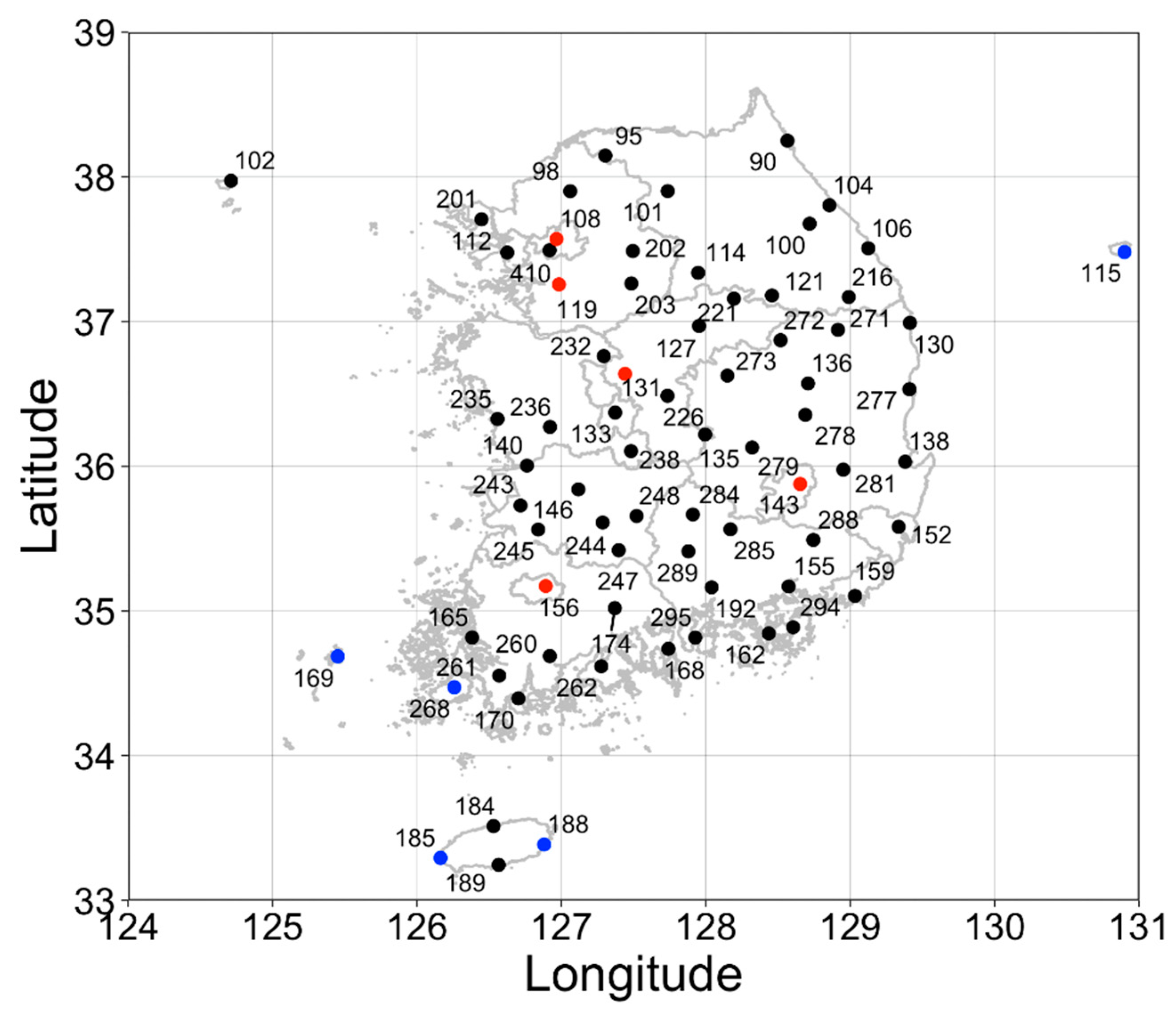
ASOS Observation Sites (72)
ASOS sites (24) using Biral VPF730 visibility sensor: Sokcho (#90), Cheorwon (#95), Dongducheon (#98), Incheon (#112), Ulleungdo (#115), Cheongju (#131), Daejeon (#133), Changwon (#155), Yeosu (#168), Jeju (#184), Seongsan (#188), Seogwipo (#189), Ganghwa (#201), Boeun (#226), Cheonan (#232), Buan (#243), Namwon (#247), Jangheung (#260), Haenam (#261), Mungyeong (#273), Yeongcheon (#281), Geochang (#284), Miryang (#288), and Sancheong (#289)
ASOS sites (48) using Vaisala PWD22 visibility sensor: Daegwallyeong (#100), Chuncheon (#101), Baengnyeongdo (#102), Bukgangneung (#104), Donghae (#106), Seoul (#108), Wonju (#114), Suwon (#119), Yeongwol (#121), Chungju (#127), Uljin (#130), Chupungnyeong (#135), Andong (#136), Pohang (#138), Gunsan (#140), Daegu (#143), Jeonju (#146), Ulsan (#152), Gwangju (#156), Busan (#159), Tongyeong (#162), Mokpo (#165), Heuksando (#169), Wando (#170), Suncheon (#174), Gosan (#185), Jinju (#192), Yangpyeong (#202), Icheon (#203), Taebaek (#216), Jecheon (#221), Boryeong (#235), Buyeo (#236), Geumsan (#238), Imsil (#244), Jeongeup (#245), Jangsu (#248), Goheung (#262), Jindogun (#268), Bongwhoa (#271), Yeongju (#272), Yeongdeok (#277), Uiseong (#278), Gumi (#279), Hapcheon (#285), Geoje (#294), Namhae (#295), and KMA (#410)
CAMS Forecasting Variables (9)
Sea salt (μg/ m 3 , SS), dust (μg/ m 3 , DU), organic matter (μg/ m 3 , OM), black carbon (μg/ m 3 , BC), sulfate (μg/ m 3 , SU), O 3 (μg/ m 3 ), NO 2 (μg/ m 3 ), SO 2 (μg/ m 3 ), and CO (μg/ m 3 ) at 1000 hPa level
Etc. Variables (5)
Longitude (°), latitude (°), site height (m), month (1–12), and Julian day (1–365)
Table 2. Monthly comparisons of VISASOS, VISLDAPS, and VISRF (showing bias, RMSE, and R) and monthly mean data for the meteorological variable inputs in the VISRF model. Parentheses values in precipitation are the number of precipitation days.
MonthModelBias
(km)
RMSE
(km)
RVISASOS
(km)
T
(°C)
P
(hPa)
RH
(%)
WS
(m/s)
Precip.
(mm)
SSDUOMBCSUO3NO2SO2CO
(μg/m3)
1LDAPS3.595.670.5414.140.481011.754.662.070.16
(2.75)
21.482.0132.322.9011.0842.2830.1525.82491.81
RF0.612.230.91
2LDAPS5.227.160.4012.772.581010.157.972.020.31
(4.60)
18.294.8545.183.8213.7049.1031.9828.07549.96
RF0.562.360.90
3LDAPS5.357.280.4712.617.451003.860.092.280.29
(5.36)
23.417.6345.493.7715.5959.8329.8823.75553.53
RF0.192.760.86
4LDAPS3.155.690.2715.2211.901001.763.441.960.54
(6.01)
18.589.5738.043.1510.2366.7628.3621.01456.97
RF−1.142.960.79
5LDAPS1.814.750.3515.8818.26999.158.212.050.64
(4.49)
21.426.3636.993.1011.6284.5025.5119.94448.95
RF−0.782.520.78
6LDAPS4.707.170.1113.5420.97994.675.161.680.91
(6.94)
15.927.3437.843.109.1477.5526.0717.07406.24
RF−0.743.130.74
7LDAPS4.336.910.2813.2524.44994.181.181.890.93
(9.86)
25.864.5820.931.275.9764.5021.788.81260.63
RF0.183.280.75
8LDAPS3.255.860.2214.6025.72994.279.621.670.73
(7.28)
34.465.4218.950.926.0866.0526.0710.34299.69
RF0.042.910.72
9LDAPS3.215.840.3314.8821.441001.681.961.731.00
(9.83)
58.593.6614.690.843.2951.8227.2310.90267.81
RF0.173.260.71
10LDAPS2.835.310.3515.5315.501005.475.431.791.45
(4.47)
56.247.7314.040.833.2645.8526.4611.90265.93
RF0.753.030.75
11LDAPS2.615.120.3915.358.751008.869.041.740.53
(4.32)
36.5313.0818.871.043.0137.6129.2317.33320.80
RF0.352.540.82
12LDAPS3.906.030.5113.803.041011.365.761.830.24
(5.18)
23.477.5921.951.214.3638.0729.2620.09356.62
RF1.422.920.88
Table 3. Comparison of VISASOS, VISLDAPS, and VISRF in urban and island regions (show bias, RMSE, and R) and mean data for meteorological variables. Parentheses values in precipitation are the number of precipitation days.
RegionModelBias
(km)
RMSE
(km)
RVISASOS
(km)
T
(°C)
P
(hPa)
RH
(%)
WS
(m/s)
Precip.
(mm)
SSDUOMBCSUO3NO2SO2CO
(μg/m3)
UrbanLDAPS1.013.280.6314.4714.031009.064.021.730.57
(69.25)
12.388.0841.833.439.6048.0242.9534.29555.81
RF−0.262.100.85
IslandLDAPS4.235.450.4015.1914.871006.573.553.820.83
(91.25)
120.316.5712.490.857.1883.293.433.40222.70
RF0.011.740.89
Table 4. Correlation coefficients (R) between VISRF and meteorological variables. Values in parentheses are the correlation coefficients between VISASOS and the meteorological variables.
RegionTRHPPrecip.WSSSDUOMBCSUO3NO2SO2CO
Urban−0.03
(0.10)
−0.40
(−0.33)
0.24
(0.05)
−0.18
(−0.15)
0.37
(0.35)
0.21
(0.17)
−0.04
(−0.01)
−0.63
(−0.48)
−0.60
(−0.42)
−0.72
(−0.64)
−0.09
(0.01)
−0.60
(−0.47)
−0.52
(−0.38)
−0.61
(−0.48)
Island−0.37
(−0.33)
−0.72
(−0.66)
0.61
(0.52)
−0.41
(−0.34)
0.12
(0.06)
−0.07
(−0.12)
−0.04
(−0.02)
−0.31
(−0.27)
−0.33
(−0.30)
−0.39
(−0.38)
−0.22
(−0.16)
−0.11
(−0.15)
0.21
(0.10)
−0.20
(−0.22)
Publisher’s Note: MDPI stays neutral with regard to jurisdictional claims in published maps and institutional affiliations.

