Impact of Tropical Cyclones on Inhabited Areas of the SWIO Basin at Present and Future Horizons. Part 1: Overview and Observing Component of the Research Project RENOVRISK-CYCLONE

Abstract

The international research program “ReNovRisk-CYCLONE” (RNR-CYC, 2017–2021) directly involves 20 partners from 5 countries of the south-west Indian-Ocean. It aims at improving the observation and modelling of tropical cyclones in the south-west Indian Ocean, as well as to foster regional cooperation and improve public policies adapted to present and future tropical cyclones risk in this cyclonic basin. This paper describes the structure and main objectives of this ambitious research project, with emphasis on its observing components, which allowed integrating numbers of innovative atmospheric and oceanic observations (sea-turtle borne and seismic data, unmanned airborne system, ocean gliders), as well as combining standard and original methods (radiosoundings and global navigation satellite system (GNSS) atmospheric soundings, seismic and in-situ swell sampling, drone and satellite imaging) to support research on tropical cyclones from the local to the basin-scale.

1. Introduction

Due to their highly destructive potential, tropical cyclones (TCs) have long been considered a major risk for populations, territorial economies, and biodiversity. In this regard, predicting their outcome and impacts at present and future times is one of the major concerns of both the Intergovernmental Panel on Climate Change (IPCC) and the World Meteorological Organization (WMO).

As highlighted in the latest reports of WMO’s International Workshop on Tropical Cyclones (IWTC), research carried out over the last four years has considerably improved our understanding of TC intensification processes [1,2], as well as TC tracking and intensity forecasting [3,4]. The operational implementation of coupled ocean-atmosphere (OA) numerical weather prediction (NWP) systems by many national weather services has, in particular, played a key role in reducing forecasting errors at all space and time scales [5,6,7,8]. Despite these important advances, additional efforts are still needed to accurately predict and characterize the potential impacts of tropical cyclones on a given territory, especially during landfall. Such efforts include, for instance, the collection of novel atmospheric and oceanic observations, to better constrain (and verify) the performance of coupled NWP systems [9,10], as well as the implementation of wave models and specific microphysical parameterizations to improve roughness, swell, wind speed, and momentum flux representation in TC forecasting systems [11,12,13].

Accurate modelling of OA interactions is particularly crucial in areas such as the tropical south-west Indian Ocean (SWIO) basin (30–90° E, 0–40° S), where the atmospheric variability is associated with a particularly strong oceanic response (and vice versa). The SWIO (Figure 1), which contributes to approximately 10–12% of the worldwide cyclonic activity [14,15,16], is indeed widely considered as the cyclonic basin with the highest prevalence of OA interactions [17] due to the unique structure of the thermocline in the Seychelles-Chagos Thermocline Ridge area (55–70° E, 5–15° S) [18,19]. Like most TC basins, the SWIO includes many fragile countries, whose economic development and infrastructure, as well as food, medicine and water supply chains, are regularly impacted by tropical cyclones.

In very recent years, countries bordering the Mozambique Channel (MC) have indeed been struck by a series of extremely intense and devastating events, whose economic impact will be felt for many years to come. Heavy rains associated with TC DINEO (2017) have caused 700,000 refugees and tens of millions of USD of damage in Mozambique, while the overall cost of TCs ENAWO (2017) and AVA (2018), which affected nearly one million people in Madagascar, was estimated to be more than USD 600 million (about 7% of Madagascar’s average annual gross domestic product). These heavy tolls are, however, out of all proportion to those of TCs IDAÏ (considered by the United Nations as the worst natural disaster ever in the MC) and KENNETH (the most intense TC ever reported in the MC [20]), which both made landfall in Mozambique in 2019 [21]. According to the latest economic reports, these two storms have affected a total of nearly 1.7 million people and caused damage and losses estimated at ~USD three billion—plus a further recovery cost estimated at USD 3.4 billion—by the World Bank and Mozambican officials [22].

Given the colossal impact of TCs on the local populations, infrastructure, and economic development of many countries in the SWIO basin, the European Union (EU), together with the Regional Council of Réunion Island and the French State, have designed the transdisciplinary research program "Réunion NOVative research on cyclonic RISKs" (ReNovRisk), to improve the resilience of SWIO countries to TC hazards and mitigate associated economic vulnerability, damages, and risks (e.g., winds, rainfall, landslides, submersion) in inhabited areas. To achieve these objectives, ReNovRisk has been divided into four interlinked research projects, referred to as ReNovRisk-Cyclone, -Erosion, -Impacts and -Transfer, whose overall objectives are described in [23]. The present paper focuses on the Cyclone component of this program, which involves a large international consortium of research institutes, universities, and weather services originating from France (e.g., universities of Réunion Island and Toulouse, Centre National de Recherche Scientifique (CNRS), Météo-France, Institut de Physique de Globe de Paris (IPGP), Institut National de l’Information Géographique et Forestière (IGN), Institut Français de Recherche pour l’Exploitation de la MER (IFREMER)), Mozambique (Eduardo Mondlane and Pemba Unilurio universities, Mozambique Weather Service (INAM)), Madagascar (Institut Supérieur de Technologie de Diego Suarez, Université d’Antananarivo), the Seychelles (Seychelles Meteorological Authority, Seychelles Islands Foundation), Mauritius (Mauritius Oceanography Institute), as well as international institutions such as the European Space Agency (ESA) and WMO, among others.

Through its observing, modelling, climate and outreach components, ReNovRisk-Cyclone (hereafter referred to as RNR-CYC) aims to improve the observation and modelling of TCs, as well as to provide inputs for other components of the global ReNovRisk program focusing on hydrological (RNR-Erosion and RNR-Transfer) and economical (RNR-Impact) consequences of tropical cyclones [23]. Another key objective of RNR-CYC is to foster regional cooperation and improve public policies adapted to present and future TC risks faced by territories bordering the SWIO. The latter is all the more essential because predicted changes in the coupled OA system due to global warming are likely to generate significant modifications of the cyclonic activity in the coming decades. Consequently, regions that are currently spared or moderately affected by TCs, and that often lack experience-based adaptation strategies, may soon have to face potentially increasing TC-related hazards [24,25]. Such changes include, for instance, the widening of the tropical belt resulting from ocean warming [26,27], which has already been shown to induce a poleward migration of TC’s lifetime maximum intensity (LMI) in both hemispheres [28,29,30,31], or significant modifications in TC frequency and/or length of the TC season [32].

This paper aims to describing the structure and main objectives of the project RNR-CYC, as well as to present an overview of the main applications and results of its observation component—modelling aspects are presented in more details in the companion paper [33]. This article is organized as follows: Section 2 provides an overview of the four components of RNR-CYC (observation, mesoscale modelling, climate modelling, cooperation, and outreach). Section 3 presents the major achievements of RNR-CYC regarding oceanic and atmospheric observations, while Section 4 concludes and discusses new research topics to be investigated beyond the end of this program.

2. Structure and Objectives of RNR-CYC

The project RNR-CYC focuses on the meteorological and oceanographic impacts of TCs in the SWIO (Figure 1) at both present and future horizons. It aims, in particular, to better apprehend the impacts of these extreme storms on the main inhabited islands of this oceanic basin by providing innovative modelling and observing products that will also feed the cascade risk analysis tools deployed in the other research components of the global ReNovRisk program [23]. In order to achieve these objectives, RNR-CYC has been divided into four components (Figure 2): (i) an observation component, to improve both long-term and temporary observations of TCs and their atmospheric and oceanic environments; (ii) a mesoscale modelling component, to improve modelling and short-term forecasting of TCs; (iii) a climate component, to evaluate the consequences of climate change on the variability and structure of TCs at both local and basin scales; and (iv) an outreach component, aimed at improving capacity building in the three aforementioned research areas through strengthening cooperation between SWIO countries. An overview of the structure and objectives of these four components is described hereafter.

2.1. Observing Component

The observing component of RNR-CYC is aimed at providing additional observations of TCs and their environment by improving regional and local observing capabilities in the SWIO. It has been built around three complementary approaches:

(i) A “conventional” approach, based on the reinforcement of regional ground-based meteorological observation facilities and, in particular, of the water vapor Global Navigation Satellite System (GNSS) observation network operated by the International GNSS Service (IGS). Starting in November 2017, 10 new public observation sites (composed of ground-based GNSS receivers and collocated surface weather stations) have been deployed in Madagascar, Eparses Islands, and the Seychelles in the frame of RNR-CYC’s sub-program “Indian Ocean GNSS Applications for Meteorology” (IOGA⁴MET [34]) to increase the number of tropospheric GNSS measurements (e.g., zenithal delay, integrated water vapor amounts) and positioning data throughout the western part of the basin (see Section 3.2.2.). The first analysis of GNSS-derived observations collected during RNR-CYC have already demonstrated the benefit of these new permanent stations to investigate the water vapor cycle at diurnal to inter-annual time scales [34,35], but also to provide new and continuous observations to investigate the dynamics of the Earth’s crust in this particularly active part of the world [34,36].

(ii) An “experimental” approach, based on the temporary collection of atmospheric and oceanic observations at various locations in the basin. For this purpose, several atmospheric and oceanographic field campaigns have been organized throughout the 3.5-year duration of RNR-CYC, with the goal to provide novel datasets to evaluate numerical model developments and simulations performed in the frame of the project [33]. The main achievements include:

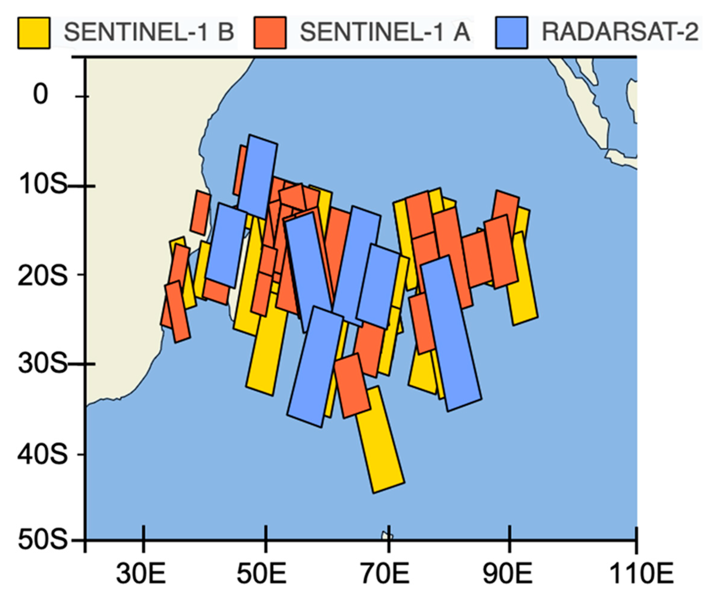
• A three-year satellite acquisition campaign (2017–2020), set up in collaboration with ESA and IFREMER, to collect high-resolution (1 km) observations of surface winds and sea roughness from spaceborne synthetic aperture radars (SARs) deployed onboard the satellites Sentinel 1A/1B of the European Earth Observation Program Copernicus (https://www.copernicus.eu/fr, see Section 3.3., accessed on 20 March 2021);
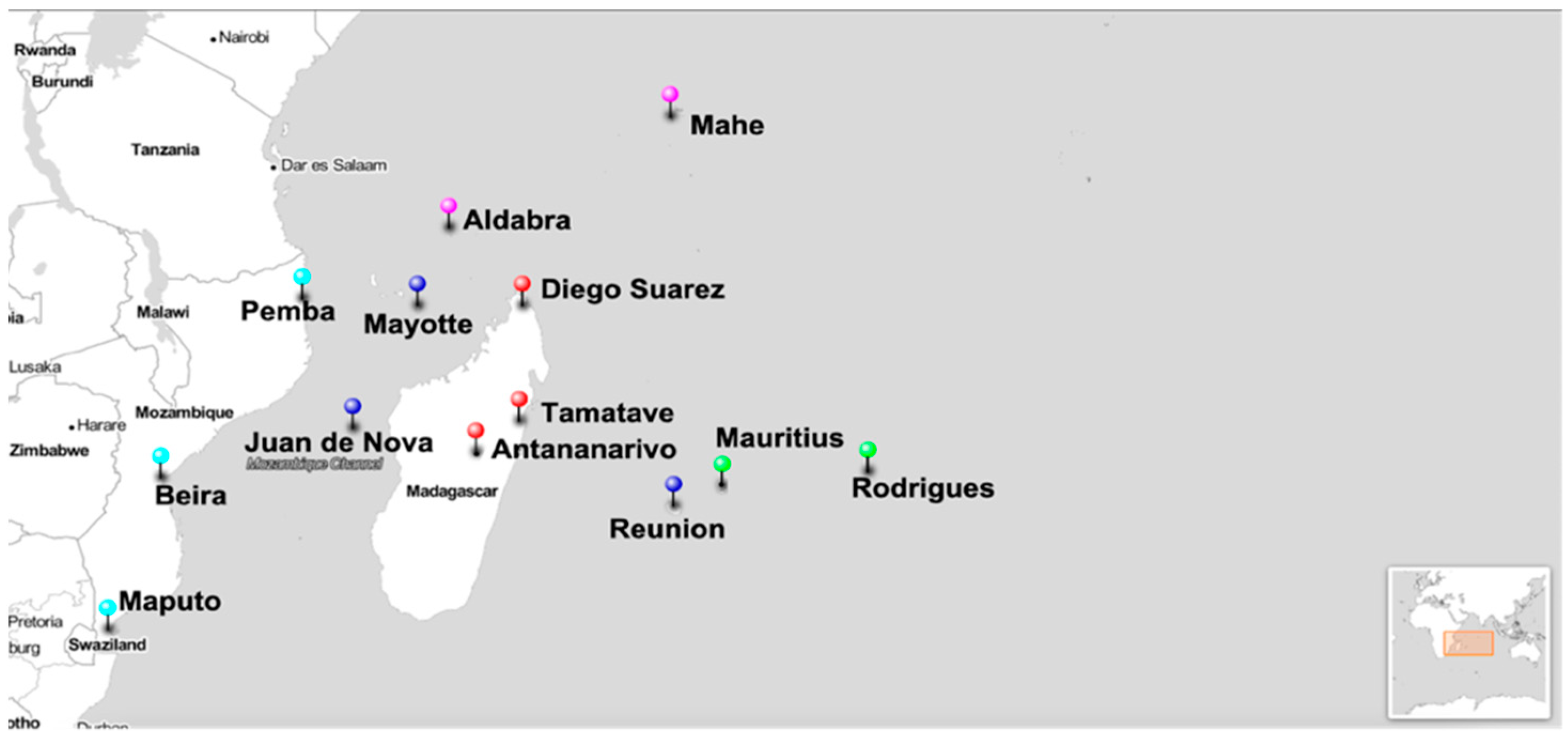
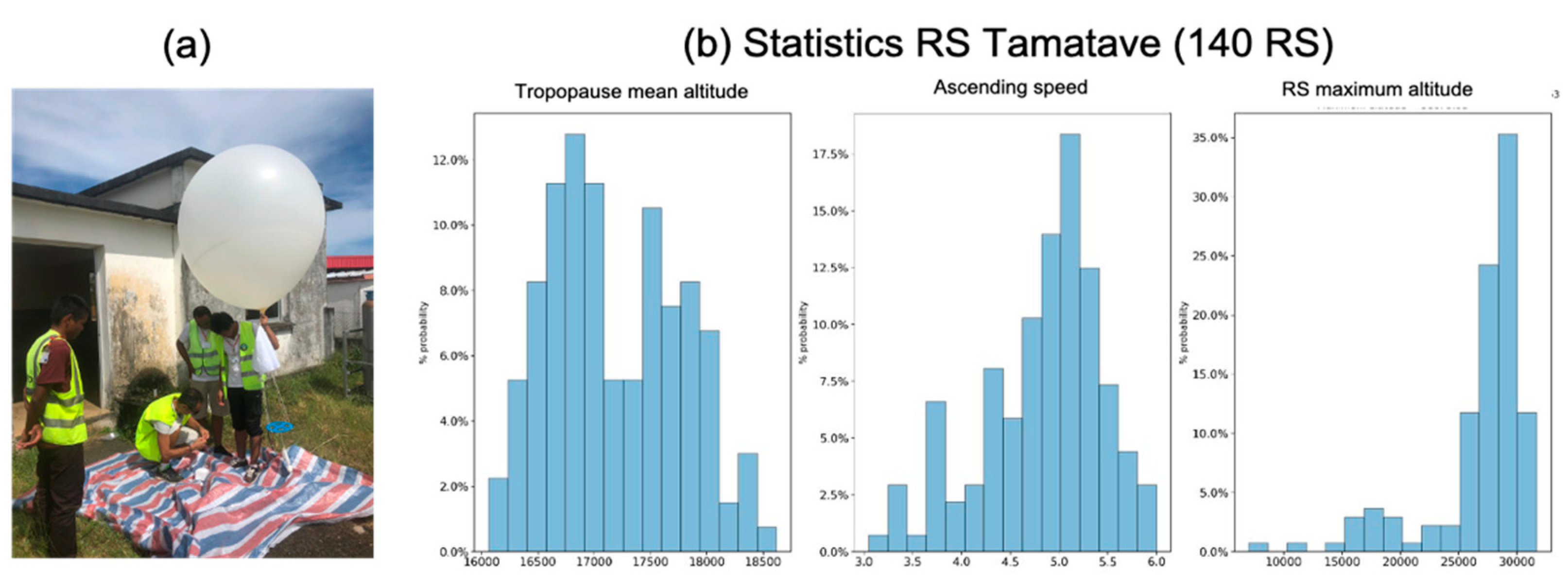
• A regional field campaign, organized from late January to early April 2019, to investigate atmospheric and oceanic environmental conditions prevailing in the vicinity of TCs during the 2018–2019 TC season. During this 2.5 month period, a regional radiosounding network, allowing for the collection of nearly 500 soundings, was deployed in Mayotte (France), Toamasina (Madagascar) and Maputo (Mozambique) to both sample the atmospheric environment of TC and train students and academics in experimental meteorology (see Section 2.4.);
• The deployment of two ocean gliders from Réunion Island to sample the vertical properties of the upper ocean layers in the Mascarene Archipelago (see Section 3.1.4.);
• The deployment of an unmanned airborne system (UAS), equipped with aerosol, turbulence, sea state, and meteorological sensors to measure OA fluxes and aerosol concentrations off the shore of Réunion Island (see Section 3.2.1.);
• The organization of several local observation campaigns to sample sea swell properties during austral winters and summers using acoustic Doppler current profilers (ADCP) and wave gauges deployed near the shore of Réunion Island (see Section 3.1.1.).

(iii) An “exploratory” approach, based on the deployment and evaluation of innovative methods to collect oceanographic observations. A particularly original approach, based on biologging technology, has been evaluated for two years to collect data from sea turtles (ST) equipped with dedicated ARGOS environmental tags in the frame of RNR-CYC’s subprogram “Sea Turtle for Ocean Research and Monitoring” (STORM, see Section 3.1.3.). Another original approach, based on the previous work of [37,38,39], was also further investigated to quantify extreme swell phenomena from microseismic noise measurements recorded by ground seismometers (see Section 3.1.2.). The preliminary assessment of terrestrial seismic observations collected in Réunion Island against oceanographic records and offshore wave model data have demonstrated that land-based seismic stations could be particularly useful to observe both austral [40] and cyclonic swell [41] (this Special Issue).

2.2. Modelling Component

Protecting life and property requires a precise estimate of the environmental changes associated with the passage of TCs in the vicinity of inhabited areas. The challenge in the face of the cyclonic threat is to simultaneously predict the track and intensity of the storms, but also the consequences resulting from their landfall, or transit near inhabited areas. Hence, damages caused to a given territory, which are essentially related to rainfall intensity, wind strength and sea state (e.g., swell), could significantly differ depending on whether it is affected by a tropical storm (TS), a monsoon depression, or a more or less intense TC. To this end, many operational meteorological services and research centers concerned with TC hazards have made considerable efforts to develop deterministic and ensemble coupled NWP systems providing high spatial resolution forecasts in all TC basins [42,43,44,45,46]). Another fundamental element to improve TC impact predictions, which is partly addressed in the hydrological component (RNR-Erosion) of the global ReNovRisk program, is to also take into account the role of land surface and hydrological processes even after the dissipation of the storm. The recent case of TC IDAÏ, whose catastrophic damage in Beira was mainly caused by flooding occurring days after the storm had passed over the city, is a perfect example of the urgent need to also improve hydrological forecasting.

Improving TC forecasting first and foremost implies a proper representation of the interactions between the storm and the ocean, and vice versa [47]. During the propagation of a TC over an oceanic area, mixing caused by surface winds usually induces a significant drop in surface temperature [48,49] that strongly reduces surface enthalpy and heat fluxes [50,51]. These air–sea fluxes can also be significantly impacted by waves, which redistribute momentum in the near-surface layer and modify the enthalpy fluxes through the emission of sea spray [52,53,54,55,56,57]. In this regard, new parameterizations reproducing the impact of marine aerosols on turbulent heat exchanges have been proposed and validated in recent years [58,59], but are yet to be implemented in atmospheric models to thoroughly evaluate their impact on TC behavior.

Radiative cooling [60,61], evaporation [62,63] and latent heat release [64] have long been recognized to play a key role in the development and intensification of tropical cyclones; therefore, particular attention must also be paid to microphysical schemes implemented in NWP systems. These schemes must, in particular, allow for an efficient representation of the radiative cooling at the top of the storms (which is a constraining criterion of TC intensity) and of the vertical distribution of latent heat (which represents the main source of energy of TCs). They should thus also be able to realistically take into account the role of atmospheric aerosols, that (indirectly) affect the radiation balance by impacting on the radiative and precipitating properties of the clouds. Improving TC forecasting therefore also implies the development of coupled aerosol–microphysical–radiation schemes to be integrated in fully coupled ocean–wave–atmosphere (OWA) models.

An important objective of RNR-CYC was to develop high-resolution OWA and OA modelling systems capable of representing, as exhaustively as possible, the multitude of physical interactions that control the variations of intensity of TCs, as well as their impacts (wind, rain, swell) at the scale of SWIO territories. The main modelling developments made in the frame of this project can be found in [11,65], (this Special Issue, [66]) and in the companion paper [33].

2.3. Climate Component

Evaluating the impact of climate change on the frequency and intensity of tropical cyclones is considered as one of the top five issues of concern by the IPCC. Currently, regional and global climate models make it possible to identify the preferred areas of cyclogenesis and occurrence of tropical low-pressure systems at the basin scale, but cannot yet be effectively relied upon to investigate potential changes in their structure and intensification mechanisms. Although it is now widely accepted that the global increase in sea surface temperatures in tropical areas will be a favorable element for TC development, it is not clear how other ingredients involved in their formation and intensification will evolve in the future. In this regard, another important objective of RNR-CYC was to evaluate the global evolution of cyclonic activity in the SWIO, but also to investigate potential structural and intensity changes of TCs resulting from the ongoing modification of their oceanic and atmospheric environments.

The modelling strategy was based on two complementary approaches, allowing to both estimate the evolution of cyclonic activity at the basin scale (i.e., changes in trajectory, intensity, and frequency of TCs at different time scales), and to assess potential structural changes and impacts of TCs at the local scale. This strategy relies on the exploitation of unprecedented high-resolution global climate simulations [32], as well as of mesoscale coupled simulations to estimate the impact of climate change on the intensity, behavior, and consequences of TCs at the scale of a given territory. Examples of results obtained from such high-resolution model runs are discussed in [33,67] (both in this Special Issue).

2.4. Regional Cooperation

Another important objective of RNR-CYC is to provide enhanced tools and knowledge to SWIO countries facing cyclonic hazards. Responding to this strong societal issue requires a better structuring of the regional scientific community, as well as significant reinforcement of the cooperation between countries bordering the SWIO basin. While regional collaboration already exists through WMO’s regional structures (e.g., Tropical Cyclone Programme (https://public.wmo.int/en/our-mandate/focus-areas/natural-hazards-and-disaster-risk-reduction/tropical-cyclones, accessed on 20 March 2021) and Réunion Island’s Regional Specialized Meteorological Center (RSMC La Réunion, http://www.meteo.fr/temps/domtom/La_Reunion/webcmrs9.0/anglais/index.html, accessed on 20 March 2021)) and the Indian Ocean Committee (https://www.commissionoceanindien.org/, accessed on 20 March 2021), interactions remain essentially focused on operational and technical applications, and only modestly promote research development in this area.

One of the strengths of RNR-CYC consists of the implementation of a partnership involving many regional research institutes, universities, and meteorological services that agreed to pool their resources and expertise to strengthen the resilience to TC hazards, and develop public policies better adapted to the risks faced by SWIO territories. RNR-CYC is thus a fundamentally collaborative project that is not only based on the large sharing of data and experiences, but also on training programs and capacity-building initiatives in the fields of observation and forecasting. These actions include, for instance, the organization of forecasting training sessions at RSMC La Réunion, of training courses in climatology and climate change, as well as numerous co-supervised MSc internships based on the analysis of experimental measurements collected in the project.

For instance, the project’s field phase, which involved nearly one hundred participants from late January to mid-April 2019, was an opportunity for many students and researchers to initiate themselves to the technique of atmospheric radiosounding (RS). During this 2.5-month campaign, ~500 radiosoundings were performed from three experimental sites specifically deployed for this occasion in Maputo (INAM’s headquarters, Mozambique), Mayotte (Météo-France weather center, France), and Toamasina (Toamasina international airport, Madagascar). On this occasion, nearly 60 students and academics from Antananarivo (Madagascar), Eduardo Mondlane (Mozambique) and Réunion universities came to Toamasina and Maputo to conduct RS measurements, while many senior forecasters of INAM and Météo-France Mayotte had, for the first time, the opportunity to operate and familiarize themselves with an RS station (Figure 3).

The involvement of the French consular services in the project also made it possible to communicate widely to the general public, the scientific community, and the media in Mozambique, Madagascar and the Seychelles on the issues of adaptation to climate change and natural hazards. As will be seen in Section 4, these regional collaborations will continue for many years to come through several new research projects initiated by RNR-CYC.

3. Results

3.1. Oceanic Observations

3.1.1. In Situ Swell Observations

One of the main objectives of RNR-CYC is to assess the impact of tropical cyclones on land, including possible submersion resulting from cyclonic swell surge along coastlines. In many tropical islands, the latter are bordered by coral reefs that can serve as a defense against flooding. These reef systems, particularly fringing reefs, protect the coastline by acting as low-pass filters that can reduce the energy of wave flows reaching the coast by up to 98% in the gravitational part of the wave spectrum [68]. The physical processes underlying coral reef coastal protection consist of a complex combination of incident waves, tides, and wind-induced surges [69,70,71].

Ocean wave energy is concentrated in the gravitational frequency band of the wave spectrum, generally between 0.04 Hz and 0.25 Hz. These gravitational waves (GWs) are the main drivers of the hydrodynamics of reef systems, as well as of beaching, runup, and submersion. During and after breaking at the edge of reef systems, GWs are dissipated while low frequency waves (infragravity waves (0.004 < IG (Hz) < 0.04) and very low-frequency waves (0.001 < VLF (Hz) < 0.004) propagate to the shore. Previous analyses of these propagation and transformation processes across various coral reefs have shown that wave dynamics could vary considerably depending on the characteristics and location of reef systems [71,72].

In order to both quantify the physical processes linked to severe sea states and assess the protective role of reef systems, a cross-shore transect, composed of bottom-fixed wave gauges and ADCPs, was deployed in Réunion Island from February to April in 2019 and 2020. Instruments were installed at the fringing reef of “Trou d’Eau”, located along the west coast of the island (Figure 4a). At the near-shore site, reef-base (RS) and reef-flat (RF) stations were deployed through the fringing reef along a cross-shore transect. The RS station was installed at the base of the reef slope at an average depth of 12 m, while three RF stations (RF1, RF2 and RF3 in Figure 4a) were aligned on the flat reef inside the lagoon at a depth of 1 m (Figure 4b,c). RS and RF stations were all equipped with synchronized ocean sensor system instrument (OSSI) wave gauges, enabling continuous recording pressure at a sampling frequency of 10 Hz. The RS station also featured an upward-looking Nortek AQuadopp (AQP) profiler configured to measure current profiles every 20 min, with a 2 Hz hourly burst mode to record wave parameters. In 2020, an ADCP (RDI Sentinel V100) was also deployed at an ocean offshore (OC) site at a depth of 45 m. This instrument was configured to record incident wave parameters from hourly bursts of 2100 samples at 2 Hz, and current profiles from the bottom to the surface.

Observations collected at the offshore stations OC and RS were relied upon to describe and quantify the main properties (height, period, and direction) of the waves impinging on the reef in the GW frequency band (wave periods ranging from 4 to 25 s), while data gathered at RF stations were used to investigate wave transformation (across the fringing reef) and propagation (from outside the lagoon to the shore). Observations collected at OC and RS stations were processed with the RDI software “Velocity” and the PUV method [73], respectively. All OSSI pressure data were corrected from atmospheric mean sea level pressure data recorded at the surface weather station of “La Rivière Des Galets” (located 20 km northward of the experimental site, RDG on Figure 4a) and non-hydrostatic pressure following the linear wave theory [74].

The mean surface elevation was computed from a 20 min moving average of the signal, while the wave spectrum and average wave parameters were obtained through the application of a fast Fourier-transform (FFT). The latter was applied over 4096 data points for incident gravity wave band or swells (0.04 < SW < 0.25 Hz), and 32,768 data values for infragravity (0.004 < IG < 0.04 Hz) and very low frequency (0.001 < VLF < 0.004 Hz) bands. The recorded signal was not perfectly periodic; therefore, a Hamming window, leading to zero value at the edges, was also applied to mitigate artifacts resulting from leakage issues. To avoid resulting loss of information at the edges, a 30-min (resp. 3 h) time average was then performed for the incident (resp. IG and VLF) bands. Time series of power spectra density deduced from data collected in 2019 along the cross-shore transect are shown in Figure 5, together with the associated mean power spectra at each station.

Measurements collected at the reef slope station RS clearly show that the wave energy spectrum is concentrated in the gravity band, with an averaged peak period of 13.5 s over the whole period. After breaking at the reef crest, most of this energy is dissipated (by breaking and/or by friction on the reef bottom), while the remaining part (in IG and VLF bands) is transferred inside the reef system. For the two strong wave events observed in February (likely associated with TC GELENA to the north of Réunion Island) and April 2019 (austral swell event), the total wave energy reduction between the reef slope station RS and the adjacent reef flat station RF3 reaches 98%, a value in good agreement with previous meta-analyses [68]. Within the reef, the transfer of the remaining energy between the three stations was nevertheless slightly different for these two events. In February (TC event), the wave energy reduction reached 64% from RF3 to RF2 and 2% from RF2 to RF1, but only 47% from RF3 to RF2 and 15% from RF2 to RF1 in April (austral swell event). The main difference between these two events is related to the period of the incident waves (11.8 s for the TC-related event and 16 s for the austral swell event); this result suggests that the generation and propagation of IG waves inside the reef might be less important for short waves, induced by the wind, than for longer-period swells. This shoreward propagation with less energy reduction is also noticeable in the average spectra, which show a small translation of the peak frequency toward higher frequencies in the IG band, between the RF2 and RF1 station, and a reduction in the peak amplitude.

These preliminary analyses show that Réunion Island’s fringing reef plays a strong role in protecting the shore against incident waves. Further investigations will be conducted in order to thoroughly investigate the physical processes and the role of both reef topography and roughness on the dynamics of IG waves. This includes, for instance, the impact of shoreward-propagating IG waves on onshore suspended-sediment transport [75], and the relationship between long wave propagation (and transformation) across the reef and sea water level above the reef—the remaining long waves propagating through the reef have been shown to increase the back-reef set-up and beach runup, which could lead to increased coastal erosion during extreme events such as tropical cyclones or strong storms [76,77].

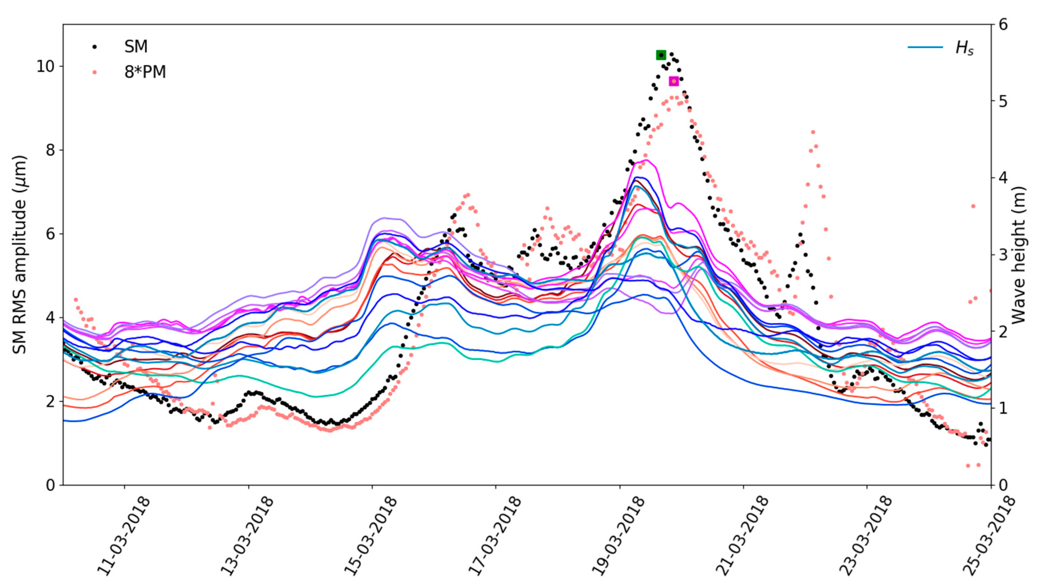
3.1.2. Ground-Based Swell Observations

The global monitoring of swell activity induced by tropical storms (TS) and TCs is of major interest to quantify the risk associated with extreme swells, but also to validate numerical models used to predict ocean activity. Direct swell observations such as those presented in the previous section are, however, strongly limited by the low number of oceanographic sensors available in this area, as well as by their deployment (and servicing) costs and their vulnerability during tropical cyclones. These limitations motivated the use of indirect observations as alternative and complementary observables to quantify the swell parameters. In this regard, the analysis of wave-induced seismic noise is known to be an interesting substitute for monitoring ocean activity and has been proven to be particularly relevant for assessing the impact of waves on coastal environments [38]. The possibility to derive swell measurements from the seismic noise generated by ocean swell and transmitted to the solid earth as seismic waves recorded by terrestrial seismological instruments [78], is discussed hereafter from data collected in RNR-CYC.

Microseisms recorded by seismic stations worldwide are known to be generated by ocean gravity waves [79]. Seismic energy spectra at terrestrial seismic stations showed two clear peaks in separate frequency bands, known as primary and secondary microseisms (hereafter named PM and SM, respectively), originating from different physical processes involving local or distant sources of ocean wave activity [80]. Primary microseisms (PM) are mostly visible at coastal and island stations and are assumed to be generated by direct interactions of swell-induced pressure variation with the coastal seafloor [81,82,83]. PM noise has the same periods as the ocean swell (i.e., between 8 and 20 s), providing a powerful way to characterize the local impact of swell approaching the shore. On the other hand, SM noise is generally generated in the deep oceans and at larger distances from coastal areas [37,84,85,86]. It dominates seismic noise at both continental and oceanic stations and exhibits a large peak at half the period of ocean waves (i.e., between 3 and 10 s), generated by the interference of swells of similar periods travelling in opposite directions [79] and generating seismic surface waves travelling horizontally within the solid crust.

In the Indian Ocean, most remote sources of seismic noise are located in the southernmost part of the Austral Ocean basin and are associated with storm systems moving around Antarctica [84,87,88]. Some noise sources may also develop at tropical latitudes in association with tropical cyclones [41] (this Special Issue). Recent seismic deployments on the ocean floor enabled the making of in situ observations of SM underneath TCs in the neighborhood of Réunion Island [37] and confirmed the possibility to track TC and TS from the ocean bottom. Although SM are generally created by distant storms, they can also be generated by the coastal reflection of waves if incident and reflected waves propagate in opposite directions [89,90]. In this latter case, the incoming swell may interfere with its reflected swell, resulting in the generation of standing waves close to coastal areas that oscillate at twice the frequency of the propagating wave [91]. Some studies suggest that local and distant sources of noise in the SM frequency peak may coexist [39,92,93].

Previous seismic analyses conducted in the Pacific and Indian Oceans have already demonstrated that several swell parameters can be derived from the seismic data. This includes: (i) the swell peak period Tp, derived from the dominant frequency of the PM and SM using the power spectral density analysis of the seismic records; (ii) the local or distant wave significant height Hs (in the case of the PM or SM band, respectively), obtained by measuring the microseism amplitudes through hourly Root Mean Square (RMS); and (iii) the wave peak direction Dp for the case of the PM band, or the source direction in the case of the SM band, which can both be deduced from the polarization analysis of the three seismic data components, to determine the dominant direction and strength of the recorded microseismic noise.

To illustrate this innovative approach, we analyse hereafter seismic observations collected during the tropical storm (TS) ELIAKIM that developed in March 2018. This storm has clear signatures, despite not reaching tropical cyclone intensity, and developed at a large distance from Réunion Island, demonstrating the potential of the method in quantifying remote systems. As mapped on Figure 6a, TS ELIAKIM started as a depression located north-east of Madagascar on 13 March 2018. It then intensified to a tropical storm on 14 March and to a strong tropical storm on 15 and 16 March while approaching the eastern coast of Madagascar, where it made landfall on 17 March. TS ELIAKIM continued its southward motion and returned over the ocean on 18 March. After a final burst on 19 March, the storm collapsed on 20 March, while entering its extratropical transition phase.

Our analysis was performed from data recorded by seismic stations of the permanent seismic network of the Piton de la Fournaise Volcano Observatory (OVPF, seismic code PF, red triangles on Figure 6b) and from a temporary seismic network deployed in the frame of the RNR program (code ZF, blue triangles on Figure 6b). Seismic data were compared with swell parameters issued from the WaveWatch3 (WW3) model [94,95] at nodes surrounding the island from the global wave model hindcast [96], indicated by stars on Figure 6b.

The seismological energy content of the vertical ground displacement of station MAT (Figure 6b) is shown in the spectrogram of Figure 7a. It displays the temporal variation of the Power Spectral Density (PSD) during the period 10 to 25 March 2018 over the frequency band of the ocean activity (0.05–0.5 Hz, i.e., 20–2 s periods). Superimposed to the spectrogram is the distance curve of the storm center to Réunion Island (dashed line), together with the storm intensity curve (black line indicating the mean wind speed and the colored dots the storm classification, as in Figure 6a). The seismic energy at this station shows good correlation with the storm intensity, despite its large distance, varying from 500 to 1500 km with two pulses of energy with the maximum at a frequency range of 0.1–0.3 Hz, i.e., in the SM band, culminating on 16 and 19 March during maximum storm intensity. Below 0.1 Hz, i.e., in the PM band, the PSD still displays clear energy increasing during the two storm peaks.

The hourly RMS amplitudes of the seismic noise recorded at the various seismic stations on the island are shown in Figure 7b,c, for both the SM and the PM bands, respectively. Note that the vertical axes are different, and that the SM amplitude is almost one order of magnitude larger than the PM. The 21 seismic stations analyzed over Réunion island display similar variation patterns. This indicates that this noise is not a purely local source; the storm acting as a distant SM source, or that the source—if local—is larger than the size of the island, which is the case for the swell generating the PM. The observed station-to-station variability in RMS amplitudes suggests the influence of local site effects such as the installation, the coupling of the seismic sensor with the ground, the nature of the bedrock, and the attenuation around the station.

The RMS peaks at seismic station MAT (Figure 7b) are observed on 16 and 19 March. This period corresponds to the maximum intensity of TS ELIAKIM and to the local variation of the swell height, as visible on Hs data issued from the WW3 model at various points around Réunion island (Figure 8). The maximum Hs observed on 19 March (corresponding to the nodes at the longitude of 55° E) interacted with the local bathymetry slightly later, which explains the small delay with the PM. A small peak was also observed on 21 March in both SM and PM data with dominating energy at period ~10s, likely originating from a distant source and not related to any local swell activity increase.

If one accepts that the SM is generated in the vicinity of the storm center and that the PM is generated in coastal areas closer to the seismic stations, one should observe a delay between the two curves. Such a delay was previously observed for austral swells generated by distant storms [40] and proposed as a precursor for predicting coastal submersion in Réunion island. In the present case, considering the involved distances (TS ELIAKIM was located ~800 km of the coast of Réunion Island on 16 March, and 500 km on 19 March) and the involved velocities (3 km s⁻¹ for the surface waves carrying the SM signal, and ~50 km h⁻¹ for the long period waves at the surface of the ocean), one should expect a delay of >10 h for each peak. However, Figure 8 shows a delay of only ~4 h between the SM and PM. This may indicate that the SM is not generated at the storm center, but likely closer to the island. Alternatively, it may also indicate a slow wind–wave growth that may take from a few hours to few days [97]. The swell–noise amplitude correlation can be used to build a transfer function to translate the amplitude of the seismic noise in terms of swell height. Although such a relation is station-related, and therefore not universal, it was nevertheless shown to provide particularly good results for strong swell events [40,41,81].

The recordings of the three components of the ground motion also make the seismic noise a vectorial observation for measuring the direction and strength of the signal polarization. In the case of the SM band, the polarization is expected to point towards the noise source, i.e., the storm center, whereas it should indicate the very local swell propagation direction in the case of the PM. In this PM case, some angle may exist between the swell propagation direction at a large distance offshore and the swell at the coast, due to refraction of the swell and the coastal bathymetry. In the case of TS ELIAKIM, the polarization was measured on an hourly basis in the SM frequency band. Figure 6b displays the average polarization recorded on 19 March at the various land seismic stations in the 0.1–0.33 Hz frequency band (pink) that can be compared to the azimuth computed from the storm center position. This map illustrates a very homogeneous orientation of the noise polarization across the island, pointing to the SW (toward the storm center location on that date) and confirming that the SM originated in the vicinity of the storm center.

These results confirm that seismic noise may provide a useful proxy to quantify the swell parameters. In the PM band (10–20 s period), the seismic noise amplitude allows for a robust quantification of the swell height Hs through a transfer function, the spectrogram allows deciphering the swell dominant period Tp, and the polarization analysis allows retrieving the local swell direction Dp. In the SM band (3–10 s period), the amplitude revealed the storm strength and the polarization indicated the storm azimuth. Terrestrial seismic stations therefore provide alternative and complementary observations of both TC and ocean activities. In some cases, the availability of several decades of seismic archives may also provide new opportunities to derive cyclone climatologies [41].

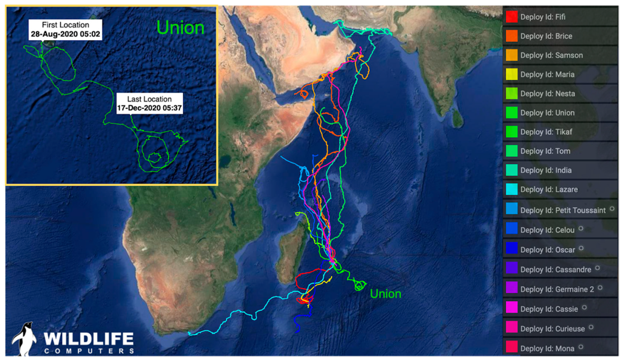
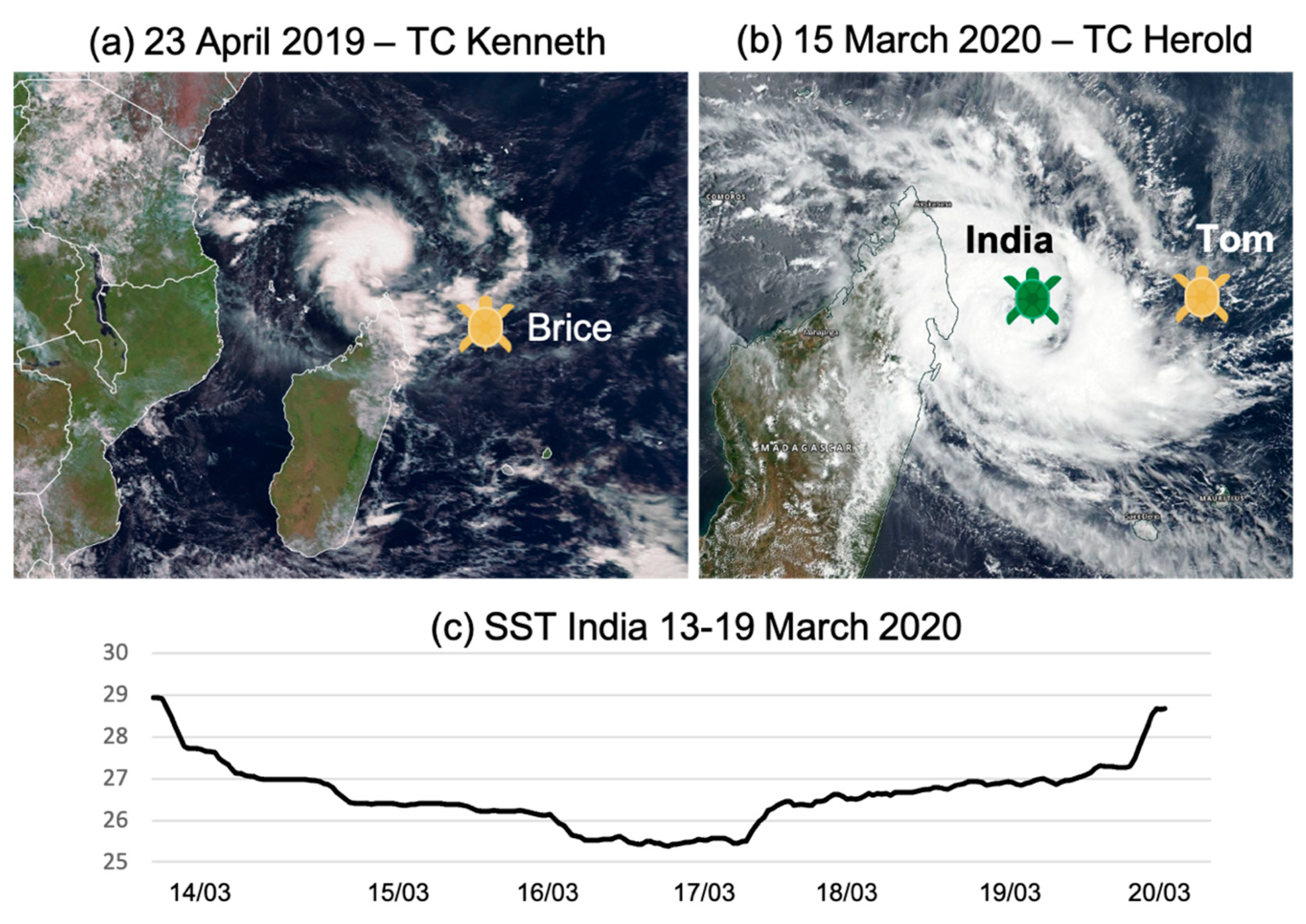
3.1.3. Biologging Observations

Observing the vertical structure of the ocean is essential to improve knowledge of both the coupled OA system and marine ecosystems. In this regard, an increasingly common alternative to gather high-resolution hydrographic profiles in the world’s oceans is to rely on animal-borne sensors (a.k.a. biologging) to collect in situ observations in remote and under-instrumented areas. Compared to conventional oceanographic in situ observation approaches (e.g., gliders, ARGO drifters, buoys, research cruises), animal-borne electronic ARGOS tags are relatively inexpensive to operate and can be deployed in remote areas with limited human resources. This approach offers all countries the possibility to actively contribute to the collection of ocean observations; therefore, biologging is expected to grow considerably in the future. The recent decision, in August 2020, of the Global Ocean Observing System (GOOS)’s Executive Committee to create a new observing network exclusively dedicated to animal-borne ocean sensors (“ANIBOS”) is definitely in line with this perspective and clearly attests of the immense potential of this approach.

The potential of biologging for sampling the thermal structure of the tropical Indian Ocean was evaluated in the frame of RNR-CYC’s sub-program “Sea Turtle for Ocean Research and Monitoring” (STORM). STORM was initiated in January 2019 by Réunion’s University and Réunion Island’s Sea-Turtle Observatory (Kelonia), with the goal of monitoring the state of the tropical Indian Ocean down to several hundred meters below the surface in near-real-time and at high spatial (<100 m) and temporal (5’) resolutions. As of March 2021, 22 animals have been equipped with Temperature–Depth (TD) ARGOS tags before being released from Réunion Island (Figure 9). Note that all animal manipulations were made by accredited ST biologists and that all STs were accidentally captured in fisherman’s nets in the vicinity of Réunion Island and brought back to Kelonia’s care center to be healed and rehabilitated.

During this experiment, two species of late juvenile sea turtles (loggerhead and Olive Ridley) were equipped with Argos TD tags. While some animals stayed in their pelagic habitats, some loggerheads also began their first homing migration to the Oman Gulf, thus enabling the collection of data both in tropical areas, from loggerheads, and subtropical areas, from Olive Ridleys (Figure 9). STs released from Réunion Island principally swam at (or slightly below) the surface (~50% of the time) and near the bottom of the ocean mixed layer (OML, ~25% of the time). They were found to dive up to 100 times a day, sometimes up to 350 m, allowing the collection of numerous hydrographic profiles within and far below the OML [9]. The analysis of data collected during the first year of this experiment has confirmed the great potential of this approach for sampling the vertical structure of the ocean, validating ocean models and spaceborne sensors, as well as to investigate the intra-seasonal variability of the tropical Indian Ocean [9].

Sea turtles are known to generally swim in rings and frontal areas in between, and often travel by moving from one ring to another [98]. These rings and eddies are numerous in the Mozambique Channel [99,100], but less common north of Réunion Island, which may explain that loggerhead STs released from there generally tend to follow a straight trajectory (Figure 9)—another explanation (currently under investigation) is that STs rarely feed during their reproductive migration, so as to reach their breeding areas as fast as possible. Nevertheless, according to its circular trajectories, ST Union (Olive Ridley), which moved south-east of Réunion Island in late 2020, apparently travelled in oceanic gyres and eddies (Figure 9).

The surface current analysis of Mercator Ocean’s operational model NEMO-PSY4 (a.k.a Glo12, [101]), averaged from 15 October to 15 December, confirmed that ST Union indeed swam in cyclonic and anticyclonic eddies of variable sizes during this period (Figure 10a). Vertical cross-sections of the ocean temperature field across the center of the main eddy (Figure 10b,c) show strong upwellings at the edges of the vortex (while downwelling can be observed at the center), resulting in significant temperature gradients at the surface (Figure 10a). This vertical transport, which brings nutrient-rich waters from the thermocline up to the surface, makes these eddies prime feeding areas for many marine species and are particularly appreciated by sea turtles. Equipping STs with environmental tags is thus an easy and relatively affordable way to sample the properties of these important transient mesoscale features, which will be further investigated in the continuation of the STORM program (see Section 4).

During this experiment, three sea turtles were also caught in the immediate vicinity of tropical cyclones during TC seasons 2018–2019 and 2019–2020: ST Brice, which moved in the vicinity of TC KENNETH (April 2019) during its cyclogenesis (Figure 11a), and STs India and Tom that were trapped in TC HEROLD (March 2020) during its intensification phase (Figure 11b). Spaceborne oceanic observations are generally unavailable under cloudy conditions; therefore, data collected by these animals also represent a fantastic opportunity to investigate the impact of TCs on the surface and subsurface structure of the ocean.

Sea surface temperature data collected by ST India in TC HEROLD from 14 to 20 March 2020 are shown in Figure 11c. During these six days, the animal remained trapped in the immediate vicinity of the storm center (~ 30 km from the TC eye) and only moved ~50 km in the north/north-west direction. In situ surface temperature observations collected from 14 to 17 March showed SST cooling of ~3.5°C (29 °C to 25.5 °C) in 72 h— during these three days, the animal remained quasi-stationary. As the storm progressively moved south-eastwards, ST India began to slowly move to the north-west, over the area previously affected by the tropical cyclone. Observations collected from 17 to 20 March showed that the temperature surface layer in this area quickly returned to pre-storm conditions, to regain its initial temperature of 29 °C on 19 March. As shown in [33], surface and subsurface observations collected by STs in tropical cyclones can also provide key data to evaluate coupled model forecasts in cyclonic conditions.

3.1.4. Glider Observations

On 22 January 2019, two SlocumG1 gliders operated by CNRS were deployed from Réunion Island for a period of two months. The two instruments were programmed to follow a north-east (glider GLNE) and a north-west (glider GLNW) trajectory to reach the northernmost region of the Mascarene Archipelago, where a high probability of TC formation was suggested about 400–600 km north of Réunion Island (Figure 12). The data acquisition strategy was set in order to complete a saw-tooth navigation pattern, allowing the gliders to dive with an angle of 26° between 5 m and 980 m depth (resulting in an along-track resolution of about 4 km once the profile was normalized on the vertical).

The two gliders were programmed to sample the ocean during descending (downcast) and ascending (upcast) profiles. Observations were transmitted in real time by satellite telemetry after each upcast, when directives for modifying the sampling strategy and glider navigation (based on operational ocean model forecasts) were also received. Each glider was equipped with various physical and optical biogeochemical instruments for sampling the ocean temperature, salinity, oxygen, turbidity, and chlorophyll-a concentration at different rates according to depth, as shown in

Table 1. Glider instrumentation, sampling rate (Hz), vertical resolution (m) and depth range (m) of collected data.

Parameter	Instrument	Sampling	Resolution	Depth
GLNE
Temperature Salinity and Depth	CTD Seabird SBE-41cp	1/8	1.5	−5 to −980
Oxygen	Aanderaa Optode 5013	-	-	-
Fluorescence Turbidity	Wetlabs flbbcd	-	-	-
GLNW
Temperature Salinity and Depth	CTD Seabird SBE-41cp	1/8	1.5	−5 to −980
Oxygen	Aanderaa Optode 4831	1/8	1.5	−5 to −980
Fluorescence Turbidity	Wetlabs flbbcd	1/8	1.5	−5 to −980

. All sensors were operational for glider GLNW, but the oxygen and optical sensors were turned off on glider GLNE.

The primary objective of this experiment was to investigate OA kinetic energy exchanges in cyclonic conditions, with emphasis on the fraction of kinetic energy transmitted to the ocean. As shown by [102], who analyzed the vertical structure of the ocean in a tropical cyclone sampled during the CIRENE field phase [103], this kinetic energy is generated on the left side of the TC track in the southern hemisphere, and later consumed by strong vertical mixing resulting from surface water cooling [104]. Due to the presence of strong currents (>0.25 m s⁻¹) along the glider trajectories, an important surface drift prevented the full application of the initially planned northward navigation strategy. The navigation parameters were then modified early in the mission to mitigate the battery consumption by reducing the depth range of the glider (because the oil pump that controls the glider buoyancy is the device that consumes the most energy). The gliders profiles were thus reduced to 500 m and 300 m depths (as shown by the colored tracks on Figure 12b,c). Real-time data transmission was also turned-off at some points to reduce the time spent at the surface, when drifting was maximized. The slower-than-expected displacement speed of the gliders prevented them from intercepting the core of TC GELENA, which developed in the area between 5 and 9 February 2019 (Figure 12a). Thanks to real-time trajectory optimization, both systems were nevertheless able to approach relatively close to the storm, as shown by black ellipses displayed in Figure 12a. For instance, glider GLNE was able to move to a distance of about 290 km from the TC center and to collect ocean data in the direct vicinity of this storm.

Vertical profiles of temperature, salinity and density collected by the two gliders between 0 and 150 m and 23 January and 17 February 2019 (along the two northward segments of the tracks) are shown in Figure 13, together with corresponding mean profiles for each parameter. The mixed layer depth (MLD), indicated by a black solid line, is estimated as the depth where the temperature differs by 0.2 °C from a surface reference value of 10 dbar [105,106]. Due to the significant distance separating the two gliders from the TC core, and because the maximum kinetic energy generated in the upper ocean occurred on the left side of the TC track, no significant change in the surface temperature could be noticed during the pre-cyclonic, cyclonic, and post-cyclonic phases (Figure 13a,d,g). A relatively constant temperature of 29 °C was observed between the surface and 30 to 40 m depth, but quickly decreased to reach 22 °C at a depth of 150 m. Salinity measurements (Figure 13b,e,h) indicated a freshening of the water within the top 100 m layer, starting around 6 February (−19.22° N) for the GLNW track, and from 28 January (−20.15° N) for the GLNE track. While part of this freshening can be explained by the rainfall generated by TC GELENA between 15° S and 5° N, another possible explanation is related to the advection of fresher water originating from the southern branch of the South Equatorial Current, which flows westward with a 20 Sv transport to feed the East Madagascar Current [107]. The velocity field computed from Mercator-Ocean’s global reanalysis model PHY-001-030, which indicated the presence of strong westward currents between 28 January and 9 February (not shown), and the vertical extent of this freshwater lens, both seem to support this hypothesis. Density measurements (Figure 13c,f,i) did not seem to be impacted by this freshening and showed a well-mixed layer within the top 40 m of the ocean and a well-stratified layer underneath.

The mixed layer depth shows significant frequency variations in relation to the diurnal cycle, and also appears deeper along the GLNW track until 8 February. GLNW was always located southward of GLNE before this date; therefore, these observations suggest a sloping up of the MLD in the northward direction. As GLNW moved northward of GLNE after 8 February, the MLD measured by GLNE became deeper, thus reinforcing the hypothesis of a northward sloping-up of MLD. A significant rise of the MLD of up to 20 m (on 5 and 6 February for GLNE and GLNW, respectively) could also be observed almost immediately after the TC formation (4 February). The MLD then returned to its initial value between 9 February (for GLNW) and 12 February (for GLNE).

The temperature–salinity (TS) diagrams collected along the full glider tracks (23 January to 23 March 2019) are shown in Figure 14. The water masses sampled by the two instruments, known as the Indian Central Water, were formed and subducted in the Subtropical Convergence area of the southern gyre of the Indian Ocean [107,108]. The OML in this water mass was generally between 50 and 150 m in depth, with temperature between 25 and 30 °C and salinity in the range of 34.9–35.4 psu. Observations collected from the bottom of the OML to 1000 m showed salinity values between 34.5 and 36 psu and temperatures decreasing from 25 °C to 5 °C.

3.2. Atmospheric Observations

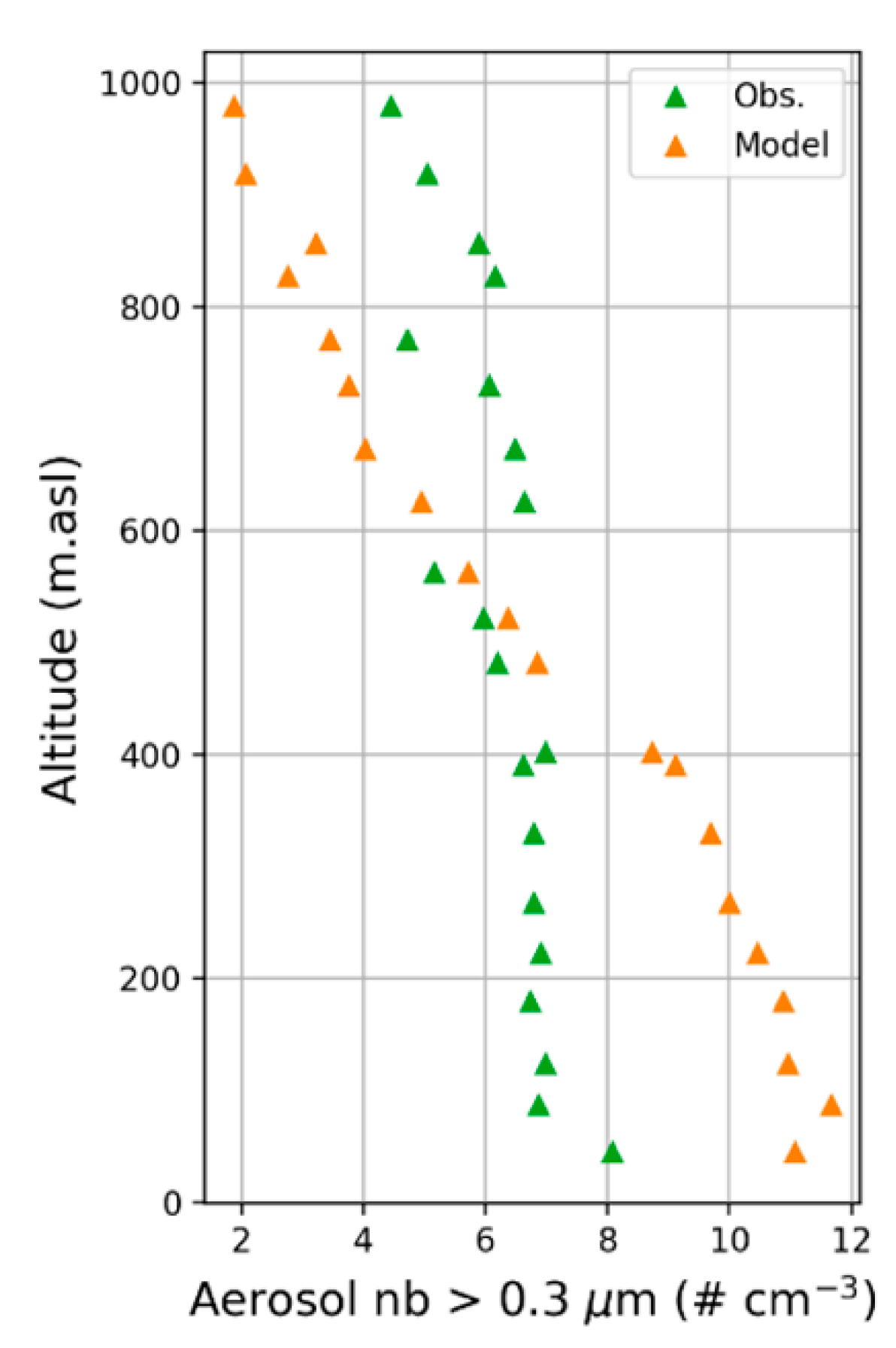
3.2.1. UAS Observations

During RNC-CYC field phase, a UAS system called “BOREAL” was operated from Réunion Island to sample the lower part of the atmosphere (Figure 15). The main objective of this experiment was to provide in situ measurements of air–sea interactions in cyclonic and pre-cyclonic conditions to evaluate numerical models and microphysical parameterizations developed in the frame of the program.

The BOREAL UAS (Boréal SAS, Toulouse, France) is a fixed-wing aircraft with a 4.2 m wingspan propelled by a thermal engine (Figure 15b) that has a maximum take-off weight of 25 kg and can fly in winds up to 25 m s⁻¹. For this experiment, a 5 kg scientific payload was developed to study air–sea interactions using an optical particle counter for measuring the aerosol number and size distribution (0.3 < diameter < 3.0 μm; MetOne), a custom-designed multi-hole probe for measurements of turbulence and three-dimensional winds, a radar altimeter for wave height and sea state measurements, a broadband shortwave pyranometer for downwelling solar radiation (Licor), an infra-red temperature sensor to measure sea-surface temperature, as well as standard meteorological measurements (atmospheric pressure, temperature and relative humidity). With this payload, the endurance and range of the BOREAL UAS was ~7 h, 700 km, and 2000 m above sea level (asl). A live video was also streamed up to 40 km from the ground-station to provide additional safety during low-altitude segments when the UAS flew ~40 m asl. The BOREAL UAS is autonomous, although its flight plan could be adapted at any time to accommodate weather conditions or air traffic via a radio or a satellite link. A transponder mounted on its wing also allowed it to integrate into international airspace.

The BOREAL UAS flew over the Indian Ocean in two exclusive zones allocated by the French aviation authority to the southeast and northwest sides of Réunion Island (Figure 15a). These two areas were dedicated for scientific flights over the international waters up to 250 km from the ground station and with a ceiling at 1067 m above sea level. BOREAL UAS operations were conducted from the airfields of Cambaie (when flying towards the north of the island) and Bras Panon (when flying towards the south). In total, 12 scientific flights were carried out between February and March 2019, for a total of 53.7 h of research flights and 5012 km of observations over the ocean. Three flights of more than 200 km from the ground station were carried out, the longest of which lasted 6 h and 18 min and covered 610 km. Examples of observations collected by the BOREAL UAS during this two-month operating period are presented below.

Figure 16 summarizes the BOREAL UAS measurements of aerosol concentrations for particle diameters >0.3 μm and >1.0 μm within 200 m above the ocean surface, compared to horizontal wind speed (Figure 16a) and wave height (Figure 16b) for conditions encountered during the two-month campaign. As expected, there was an increase in particle concentrations (diameter > 0.3 μm), which is often associated with primary marine aerosol (PMA) emissions, over the observed range of wind speed (2.2 to 13.5 m s⁻¹) and wave heights (2 to 3.7 m). However, the range of wind speeds and wave heights encountered in the vicinity of Réunion Island during the RNR-CYC field campaign remained relatively small, partly because the paths of the TCs were never closer than a few hundred kilometers to the ground station during the observed period.

Although strong cyclonic conditions were not encountered in the vicinity of Réunion Island during the 2019–2020 TC season, several BOREAL UAS flights were nevertheless impacted by the presence of TC JOANINHA, which developed in the eastern part of the Mascarene Archipelago in March 2019 (Figure 17a). The signature of this storm could be seen up to several hundred kilometers away in observations of ocean waves, atmospheric turbulence structures, and enhanced PMA emissions. These emissions, which occur over a much larger domain than the cyclonic system, have been shown to modify the TC’s track and intensity [11].

As TC JOANINHA moved to the east of Mauritius, the BOREAL UAS flew to the west of Réunion Island to sample the TC’s perimeter (see flight track in Figure 17a and wave crests, swells and clouds generated by the cyclone recorded by the on-board camera in Figure 17b). In situ measurements were used, in particular, to assess parameterizations of air–sea interactions simulated with the OWA coupled system developed in RNR-CYC (see [33] for details about this system). Results presented hereafter are derived from a coupled OWA simulation based on the ocean model Coastal and Regional Ocean Community (CROCO, http://www.croco-ocean.org, accessed on 20 March 2021), the wave model Wave Watch 3 (WW3) [94,95], and the atmospheric model Meso-NH (http://mesonh.aero.obs-mip.fr/, accessed on 20 March 2021), which was developed specifically for comparisons with the BOREAL UAS.

Figure 18 presents a vertical profile of aerosol particles conducted during the 25 March flight from near the ocean surface (<50 m asl) to above the marine boundary layer (~1000 m asl). Observed aerosol concentrations (diameter > 0.3 μm) were found to be relatively constant throughout the marine boundary layer (up to ~800 m asl) and decreased above the inversion. A surface layer with enhanced emissions, similar to the profiles observed at the surf zone in the frame of project Miriad [109], was also observed at the lowest part of the vertical profile (~50 m asl).

This surface layer, which was not captured in the model simulation (Figure 18), has not been well-documented so far and has important implications for the transport of aerosols into the well-mixed boundary layer. In addition, the simulations tend to overestimate the aerosol emissions near the ocean surface (i.e., an approximate factor of two enhancement in aerosol concentrations) and show a pronounced vertical gradient throughout the marine boundary layer with an underestimate of aerosol concentrations in the free troposphere. These large differences between observed and simulated vertical profiles of aerosol concentrations suggest that mixing timescales in the marine boundary layer may perhaps be too slow in the model—resulting in an excessive gradient in the aerosol concentration—but could also be related to a possible bias in the CAMS/COPERNICUS analyses used to initialize sea salts in Meso-NH. Although a mass distribution calculation was made to adjust the consistency of aerosol distributions in CAMS and Meso-NH, a small remaining mass difference in the finest modes can also lead to large differences in the number of aerosols, especially in areas with low primary aerosol production, i.e., where aerosol number concentrations mostly arise from initial conditions.

A few days later, a southern swell event occurred when winds shifted to the north-east direction as TC JOANINHA continued its eastward progression through the Indian Ocean. Flight operations were moved to Bras Panon and the BOREAL UAS flew along a southern curtain for more than 200 km to the east of Réunion Island on 29 March 2019 from 6:33 to 12:04 UTC (Figure 19a). The platform followed a flight plan with ascents from 100 to 1000 m asl followed by straight-level legs at 400 and 100 m asl for at least 10 km each. Mean and significant wave height observations collected during this flight by the onboard radar altimeter showed that wave height increased by about one meter (from ~2.5 to 3.5 m) between locations A and D (Figure 19b).

A similar increase in wave height was also obtained from the simulations of this case study (Figure 19a). The associated modelled (Figure 20a) and observed (Figure 20b) spectral density functions provide insight on the composition of the southern swell and show two peaks for both observations and simulations. Azimuth plots from WW3 based on the wave elevation spectrum (Figure 20c) indicate that these peaks corresponded to distinct components of the southern swell; the first component was generated by the northerly winds (red arrow in Figure 20c), and the second component was generated by TC JOANINHA to the east (black arrow in Figure 20c). In spite of the observed increase in wave height (and relatively constant wind field), a horizontal gradient in the aerosol concentration and size distribution at 100 m asl was not observed during this swell event. These results were predictable because the 1 m increase in wave height is relatively small and not expected to generate a significant difference in PMA emissions.

Due to the low number of TCs passing in the immediate vicinity of Réunion Island during the TC season 2018–2019, the range of wind speeds and ocean wave conditions were not as large as expected to fully assess parameterizations for PMA emissions. Nevertheless, the datasets collected during this campaign have clearly demonstrated the scientific potential of the BOREAL UAS, and of its associated payload, to collect key observations in remote oceanic areas and in the vicinity to tropical cyclones.

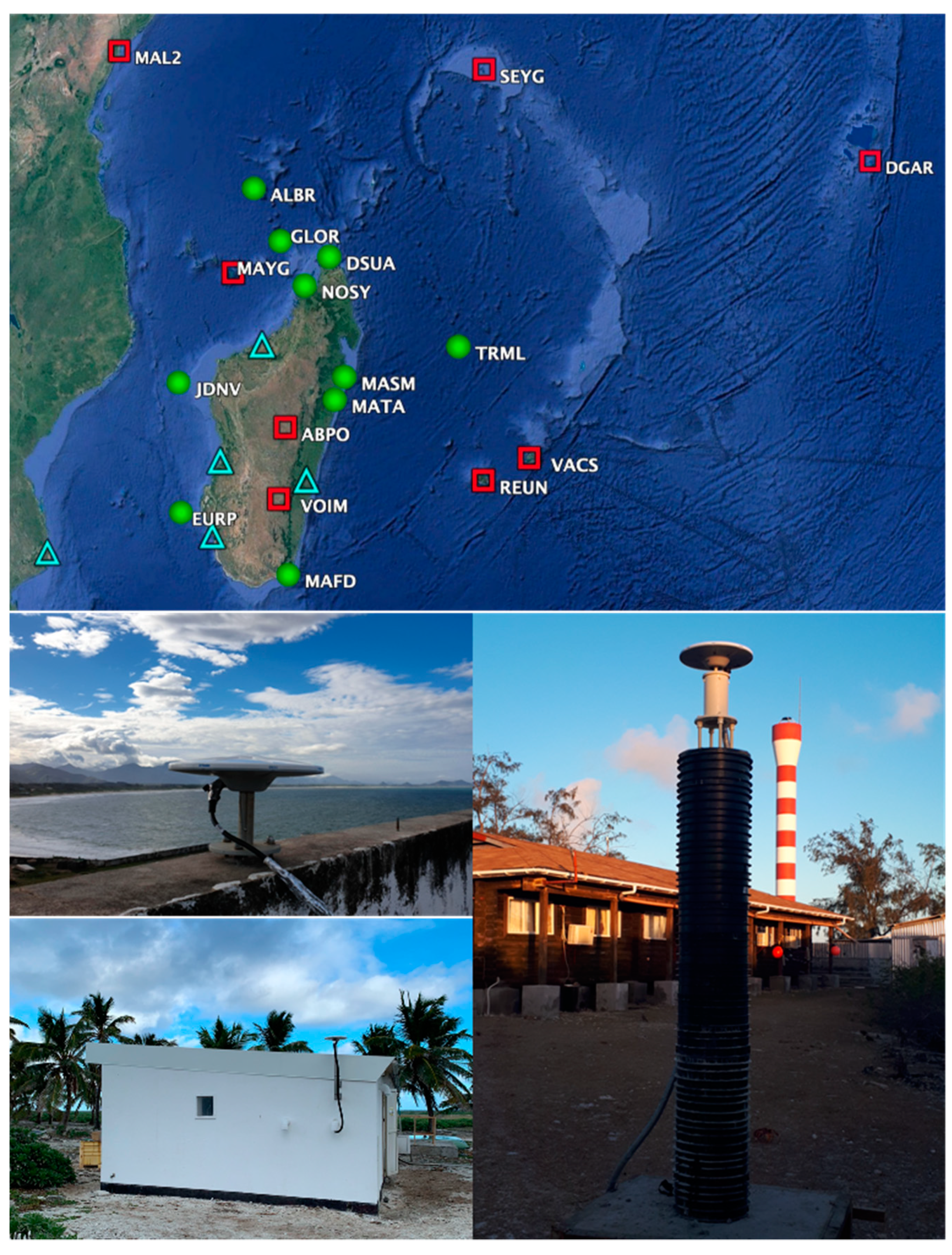
3.2.2. GNSS Observations

A well-known (indirect) atmospheric application of GNSS measurement consists of measuring the atmospheric integrated water vapor (IWV) content from the delay induced by water vapor during the crossing of the earth’s atmosphere by the GNSS signal [110]. Due to the fundamental role of water vapor in climate and weather dynamics, tropospheric GNSS measurements have rapidly become one of the main tools used by climatologists to monitor the evolution of the water vapor field at all spatio-temporal scales, but also to improve NWP model forecasts (see [111] for a recent review of current GNSS weather applications). The creation of the International GNSS Service (IGS) network in 1994 [112], which now includes more than 500 stations worldwide, has also enabled GNSS-derived measurements collected in all parts of the world to be widely disseminated to the scientific community. However, with only eight operational stations available prior to RNR-CYC (Figure 21), the density of public GNSS stations in the SWIO was the lowest of all TC basins.

During RNR-CYC, 10 new permanent stations were deployed, including one in the Seychelles (Aldabra), four in the Eparses Islands (three RNR-CYC stations at Juan de Nova, Tromelin and Europa and one shared station installed by OPGP in Glorieuses), and five in Madagascar (Diego-Suarez, Toamasina, Sainte-Marie, Nosy Be and Fort-Dauphin), with the goals of increasing the density of the GNSS network in the SWIO and to provide additional near-real-time IWV measurements at various locations in the basin (Figure 21). Although these stations have not yet been included into the IGS network (pending), most collected GNSS observations are transmitted at hourly time steps to IGN’s data center, which already allows for routine real-time GNSS calculations and the wide dissemination of derived meteorological and geophysical products through IGN’s permanent GNSS network (RGP, ftp://rgpdata.ign.fr/pub/gnssmayotte, accessed on 20 March 2021).

These new stations have already been shown to represent a fantastic asset for monitoring the spatio-temporal evolution of the water vapor field at local and regional scales [34,35], as well as to evaluate NWP forecasts [34]. A further modelling application is shown in Figure 22, which presents differences between GNSS-derived IWV observations and daily 6 h analyses of AROME-IO operational NWP systems [42] at 00:00, 06:00, 12:00, and 18:00 UTC at Aldabra (ALBR, The Seychelles), Antananarivo (ABPO, Madagascar), Réunion Island (RUN, France) and Sainte-Marie (MASM, Madagascar) during the year 2019. In order to evaluate the performance of the model at various time scales, 30-day (red), 10-day (yellow) and 3-day (black) moving averages were applied to both the model and GNSS data. GNSS observations were processed following the approach proposed by [35].

Whatever the time scale, the bias error remained relatively constant at Sainte Marie (MASM, approximately −0.3 kg m⁻²), Réunion (REUN, approximately 0.5 kg m⁻²) and Antananarivo (ABPO, approximately −2 kg m⁻²), but showed more variations in Aldabra (ALBR, between 0.6 and 1.14 kg m⁻²). Model–observation differences did not show a clear seasonal dependency, except at Aldabra where maximum errors were observed in the middle of the winter, spring, and fall seasons. In the case of this atoll, consisting of land strips of 1–3 km width encircling a lagoon of nearly 30 km × 15 km, the land is considered as submerged by the model, which does not allow taking into account the effect of vegetation and of the diurnal cycle on the atmospheric moisture content. At Aldabra, atmospheric moisture changes in the model thus mostly depend on the variation of ocean temperatures. Interestingly, the sign of the bias error is location-dependent, suggesting that the model is not affected by systematic errors. The associated standard deviation errors also tends to decrease with the length of the smoothing period, because the latter minimized the impact of short-term variations. At short time scales (three days), one can notice that the strongest discrepancies mostly occur during the TC (wet) season (days 1–120 and 330–365), in relation with the passage of tropical cyclones in the vicinity of the GNSS ground-based stations.

As already pointed out by [34], who investigated the seasonal variations of AROME-analyzed IWV errors at Diego-Suarez (DSUA), model–observation differences seem exacerbated for stations located in the vicinity of complex orography. Except for the particular case of Aldabra, the same behavior can be noticed here for the high-altitude stations of Réunion (600 m asl, REUN) and Antananarivo (2000 m asl, ABPO), which showed higher errors than for the flat island of Sainte-Marie (MASM). These errors might be related to the difficulties of the model to properly capture the modifications of air masses caused by the orography (lifting and subsiding motions) at the local scale due to an insufficient resolution of its topography. A possible way to correct for such errors could be to assimilate GNSS observations (zenithal delays) into the model. While the operational version of the AROME-IO NWP system does not allow for data assimilation, its research configuration includes a 3D-Var scheme that can be used to perform assimilation experiments [34]. Some studies are currently ongoing to determine whether the assimilation of observations collected from these new GNSS stations can help to reduce this moisture bias.

3.3. Spaceborne Observations

Visible and infrared satellite observations have long been the main source of knowledge for estimating some of the parameters (e.g., radius of maximum wind, various wind radii) characterizing the structure of tropical cyclones—these parameters are, in particular, inputs of the Dvorak method [113], used by TC forecast centers to produce best-track data and issue TC advisory and forecasts. Since the launch of the first Earth observation satellite in the early 1970s, the quality of ocean surface wind estimates in the vicinity of TCs has constantly been improved.This includes, for instance, the deployment of wind scatterometers [114,115] as well as of multifrequency radiometers [116,117] that both allow for a direct, and more precise, estimate of surface winds under TCs. More recently, a new generation of microwave radiometers has also been put into operation by ESA and the National Aeronautics and Space Administration (NASA) in the frame of the Soil Moisture and Ocean Salinity (SMOS) and Soil Moisture Active Passive (SMAP) space missions, respectively. Thanks to their large coverage and revisit times, these new sensors, which allow for high-resolution (~40 km) surface wind speed sampling in all weather conditions, provide a unique description of TC structure during its whole lifetime [118], and have thus become a key source of information for TC forecasting centers.

In addition to these more or less conventional sensors, a new approach, based on the use of spaceborne synthetic aperture radars (SARs), is also being increasingly used to probe and quantify sea surface properties under extreme wind conditions. Designed in the mid-1990s, SAR systems were initially used for land applications [119], especially for monitoring earth deformation rates ranging from a few millimeters per year (e.g., for glaciers) up to 1 m per h (e.g., earthquakes and landslides). SAR potential for marine applications was already known since the launch of the first SAR satellite [120], but has significantly emerged with the launch of the Canadian Space Agency (CSA)’s RADARSAT-1 (1995) and ESA’s Envisat (2002) satellites. Thanks to their unique capability to gather very high-resolution (up to a few meters) surface wind and roughness data in swaths of several hundred kilometers, spaceborne SARs have become key observing systems for monitoring, forecasting, and investigating the properties and evolution of TCs [120,121].

The deployment of a new generation of SAR systems equipped with polarization diversity on-board CSA’s RADARSAT-2 (RS2, 2007) and ESA’s Sentinel-1 (S1, 2014) satellites has allowed further improvements in the capabilities of these instruments to accurately map the variations of ocean surface winds in TC eyes and eyewalls [122,123]. Acquisitions made by ESA’s satellites had, however, never been used to probe tropical cyclones until the implementation of the Satellite Hurricane Observations Campaign (SHOC, 2016–2017), in the Pacific and Atlantic basins. The intercomparison of aircraft reconnaissance wind data against S1 SAR measurements collected in CAT-5 hurricane IRMA (2017) during this experiment definitely demonstrated the capability of these instruments to thoroughly describe TC ocean boundary layer structures at high spatial resolution [124].

The extension of the SHOC program to the SWIO basin (referred to as SHOC-V2) was initiated in 2017, under the frame of RNR-CYC. SAR missions cannot continuously acquire wide swaths of data in high-resolution modes; therefore, a dedicated acquisition procedure was set up to collect data without impacting the operational duty cycle of the satellites. Acquisition requests were passed along to both MDA (MacDonald Dettwiler and Associates, the private company that owns the satellite RS2) and ESA S1 mission planner portals on a 24-to-48 h notice, based on satellite orbit and five-day track forecasts provided by RSMC La Réunion. In order to reduce the workload of participating space agencies, which contributed to this experimental program on a voluntary basis, acquisition requests were also generally limited to storms presenting a threat to SWIO populations.

Between 2017 and 2021, about 150 SAR images were acquired by S1A, S1B and RS2 satellites, allowing the sampling of 20 tropical storms and cyclones over four TC seasons (raw S1 data are available at https://scihub.copernicus.eu, accessed on 20 March 2021). Among these acquisitions, nearly 40% were directly obtained within the eye or the eyewall of the systems (

Table 2. Number of Radarsat-2 and Sentinel-1 SAR acquisitions within the eyewall/eye (hits) of tropical storms (TSs) and tropical cyclones (TCs, ITC) that developed in the SWIO between February 2017 and 2021. * Acquisitions performed from 2021 onwards were made in the frame of the CYMS program (see Section 4).

Storm Name	Date	Hits	Storm Name	Date	Hits
Dineo (TC)	02/2017	2	Idaï (ITC)	03/2019	3
Enawo (ITC)	03/2017	1	Joaninha (ITC)	03/2019	7
Ava (TC)	01/2018	3	Kenneth (ITC)	04/2019	1
Berguitta (ITC)	01/2018	4	Lorna (TC)	04/2019	4
Cebile (ITC)	01/2018	8	Belna (TC)	12/2019	5
Dumazile (ITC)	03/2018	5	Calvinia (TC)	12/2019	1
Eliakim (TS)	03/2018	1	Diane (TS)	01/2020	1
Alcide (ITC)	11/2018	1	Francisco (TS)	02/2020	1
Kenanga (ITC)	12/2018	2	Herold (ITC)	03/2020	1
Gelena (ITC)	02/2019	4	* Chalane (TS)	12/2021	3
Haleh (ITC)	03/2019	6	* Eloise (TC)	01/2021	2

, “hits”). SAR images were collected throughout the SWIO basin (Figure 23) at various storm evolution stages (cyclogenesis, intensification, dissipation). Collected wind data were used for nowcasting and best-track data reanalysis purposes at RSMC La Réunion, model verification [33] and assimilation in NWP systems [125] (this Special Issue).

Examples of SAR-derived surface wind fields obtained through the application of the retrieval algorithm proposed by [126] are presented hereafter. The first example was taken within TC JOANINHA, which developed in the northeastern part of the Mascarene Archipelago (Figure 17a) and reached its LMI in the vicinity of Rodrigues Island on 26 March 2019, with 10 min of maximum sustained winds of nearly 60 m s⁻¹ (Figure 24a). The core structure of this system was observed seven times by the SAR systems deployed onboard satellites S1A/S1B and RS2 (Table 2) at various stages of its life cycle. Of particular interest is the image taken by RS2 on 28 March 2019 at 00:52 UTC (Figure 24b), when the system started to experience an eyewall replacement cycle (ERC). The latter, which often occurs when a TC reaches an intensity of 50 m s⁻¹, has long been recognized as one of the main mechanisms for intense TCs to intensify further [127,128]. During an ERC, outer rainbands strengthen and organize themselves into a ring of thunderstorms that progressively encircle the TC eyewall. The formation of this outer ring, usually referred to as the outer eyewall, eventually cuts off the supply of moisture and angular momentum that maintain convection around the eye, causing a weakening of the system and the eventual dissipation of the inner eyewall. The former ring is then replaced by the outer ring, which gradually contracts and intensifies, often resulting in a more intense TC than prior to the ERC.

The analysis of the SAR-derived surface wind field shown in Figure 24b clearly indicates the presence of two concentric areas of maximum wind located both around the eye and in the east-to-southeastern quadrant of the system core. The inner structure (maximum wind speed of ~50.2 m s⁻¹) corresponds to the eyewall of the storm, and the outer one (maximum wind speed of ~45 m s⁻¹) to the cyclonic rainbands progressively wrapping around the eyewall that will eventually replace the inner wall. As mentioned previously, the completion of an ERC is often followed by a re-intensification of the system. However, in the present case, such re-intensification did not occur because TC JOANINHA rapidly encountered a strongly sheared environment that caused its dissipation a couple of days later.

The second example is taken from TC IDAÏ (Figure 25), which is considered as the worst natural disaster that has ever affected Mozambique (as well as the surrounding countries of Zimbabwe and Malawi), and the deadliest storm ever recorded in the SWIO. This exceptional TC initiated as a tropical depression along the northern coast of Mozambique on 3 March 2019 (Figure 25a) that initially moved inland in the northwestern part of the country for a few days, with peak winds in the order of 10–15 m s⁻¹. On 7 March, it made a half-turn near the Mozambique–Malawi border and moved back towards the ocean. After entering the Mozambique Channel, on 9 March, the storm experienced a rapid intensification to reach intense TC intensity (10 min maximum sustained wind >46 m s⁻¹), with winds gusts estimated at up to 70 m s⁻¹ on 11 March. IDAÏ then reversed its track back for the second time in the immediate vicinity of the Eparses island of Juan de Nova (located approximately 150 km off the west coast of Madagascar) and began its southwestward progression towards Mozambique. Shortly after this half-turn, it entered into a slight weakening trend following the beginning of its ERC. Right after its completion, IDAÏ immediately re-intensified and reached its LMI on 14 March, with a minimum central pressure of 940 hPa and (estimated) 10 min maximum sustained winds of ~55 m s⁻¹. The storm then gradually weakened while progressing towards Beira, where it made landfall on 15 March at the TC stage.

Numerous acquisitions were made in this system by S1 satellites, including three images collected directly in the core of the storm (Figure 25b). Two of these hits were made over the ocean by S1A, at the stage of intense TC (11 March at 02:43 UTC and 14 March at 03:08 UTC), while a third one was made at landfall by S1B on 14 March at 16:00 UTC (because 90% of this swath occurred over land, this third acquisition is not exploitable). SAR wind data shown in Figure 25 are the only high-resolution wind observations collected during the oceanic phase of this system—WMO’s JDN weather station broke down a week before the passage of the storm over the island and the weather station deployed at Beira in the frame of RNR-CYC was lost during landfall—therefore, these observations represent an invaluable asset for accurately assessing numerical model simulations of this storm [33].

SAR data collected in IDAÏ and other tropical cyclones can also meaningfully complement best-track (BT) data produced by RSMC La Réunion. According to RSMC La Réunion best-track, TC IDAÏ reached its LMI on 14 March 2019 at 00:00 UTC with maximum winds of nearly 55 m s⁻¹. This value is in good agreement with the maximum intensity measured by S1B a few hours later (~52 m s⁻¹). SAR data, however, show that these strong wind values were only observed in the eastern quadrant of the storm’s core, but that the average wind speed throughout the eyewall was significantly less intense and mostly comprised between 42 and 45 m s⁻¹. On 11 March, the agreement between best-track and SAR-derived wind data was less good, with maximum wind speed in the order of 50 m s⁻¹ for the BT and 60 m s⁻¹ for SAR observations. According to SAR observations, the strongest wind speed values were also more or less uniformly distributed throughout the eyewall. Hence, the comparison of the two SAR images suggests that the destructive potential, and overall global intensity of the system, was probably much greater on 11 March, despite a 10% lower maximum wind speed (50 m s⁻¹ vs. 55 m s⁻¹) in BT data.

4. Conclusions and Perspectives

ReNovRisk-Cyclone (RNR-CYC) is an ambitious international research program aimed at developing regional cooperation in the SWIO with emphasis on the observation and modeling of tropical cyclones at both current and future time horizons. The observation component of RNR-CYC, presented in detail in this paper, has enabled the collection of numerous innovative oceanic (gliders, sea-turtle borne and seismometer-derived data) and atmospheric (UAS and SAR-derived wind data) measurements, together with more conventional observations (GNSS-derived IWV, atmospheric radiosoundings, ADCP, and wave gauge swell measurements) to investigate tropical cyclones and their environment from the local to the basin scale. Its mesoscale modelling and climate components, presented in more detail in the companion paper [33], also allowed for the development of innovative modelling systems, while its outreach component significantly increased regional collaboration between SWIO countries affected by TC hazards. The innovative data collected in the SWIO during RNR-CYC have also proven particularly useful to evaluate the performance of both research and operational TC forecasting models in this under-sampled region of the world. SAR measurements, which allow for accurate evaluations of TC forecasts, can also be assimilated into NWP systems [126]; in situ and remote swell measurements can be relied upon to evaluate wave model performance; while biologging measurements are priceless to assess ocean model representation of the ocean mixed layer in cyclonic conditions.

The promising results obtained during the 3.5-year observation component of RNR-CYC have already led to the development of numerous new research projects aimed at maintaining some of these novel measurements and further reinforcing overall observation capabilities in the SWIO beyond the end of this program (July 2021). Among the principal new research projects directly arising from RNR-CYC, one can mention STORM-IO (Sea Turtle for Ocean Research and Monitoring in the Indian Ocean), ESPOIRS (Etude des systèmes précipitants de l’océan Indien par radar et satellites—Studies of Indian Ocean precipitation systems by radars and satellites), and MAP-IO (Marion Dufresne Atmospheric Program—Indian Ocean).

STORM-IO (starting May 2021) will enable the extension ST-borne measurements conducted from Réunion Island to the whole Indian Ocean (Figure 26), in collaboration with the Terres Australes et Antarctiques Françaises (TAAF) administration (in Eparses Islands of Juan de Nova and Tromelin), Kelonia (Réunion Island), and five marine reservations in Comoros (Moheli), Madagascar (Nosy Tanikely), Seychelles (Aldabra), Mozambique (Ponto di Ouro), and South Africa (iSimanliso). This transdisciplinary project, constructed in close cooperation with ST specialists and oceanographers, will extend the research initiated during RNR-CYC to: (i) investigate Indian Ocean properties and spatio-temporal variability; and (ii) improve knowledge of the ecology of the five species of sea turtles living in the Indian Ocean. A particular emphasis will be put on the observation of mesoscale eddies and coastal currents that develop in the Mozambique Channel (to assess their impact on water mass distribution, transport, and mixing, as well as their role in the dynamics of the Greater Agulhas current system), and on the assimilation of collected ST-borne data in global and limited-area configurations of the ocean model NEMO [129]. This new component of the global STORM program, which is now strongly supported by the EU, UNESCO (through the GOOS/AniBOS), CNES and CNRS, among others, will be conducted for the many years to come, and is likely to be extended to other ocean basins in the mid-term.

ESPOIRS (started in December 2020) will carry on with the densification of the GNSS water vapor observation network initiated in the framework of RNR-CYC’s sub-program IOGA⁴MET through the deployment of five additional stations in Madagascar and Mozambique (Figure 21). Some existing, or soon to be deployed, GNSS stations will also be upgraded with co-located oceanographic sensors to monitor sea level on a regional scale. In the mid-term, these instruments will be integrated into the Global Sea Level Observing System (GLOSS, https://www.gloss-sealevel.org/, accessed on 20 March 2021) network, which monitors sea level rise on a global scale, and into the IGS network, which disseminates GNSS data to the worldwide scientific community. ESPOIRS also includes an ambitious local component aimed at collecting wind and precipitation measurements in tropical cyclones with a transportable polarimetric weather radar to be deployed in Réunion Island (2021), the Seychelles (Mahe, 2022), and Madagascar (Tamatave or Diego Suarez, 2023). This weather radar component will notably focus on the impact of orography on tropical cyclones (or outer cyclonic rainbands in the Seychelles) [130], and will help to develop regional cooperation in the field of atmospheric remote sensing.

The goal of the MAP-IO program (started in January 2021) is to deploy an atmospheric and marine biology observatory in the Indian and Southern Oceans onboard the French vessel Marion Dufresne (Figure 27), operated by the TAAF administration (for its logistical needs in the Eparses Island and French Austral Territories) and IFREMER (for scientific campaigns in the IO). With the deployment of nearly 20 new sensors on-board this RV (e.g., cytometer, titrator, thermosalinograph, cytometer, titrator, NO_x, CO, CO₂, O₃ and CH₄ analyzers, GNSS, UV radiometer, CCN, photometer, weather station), observations at the OA interface and within the atmospheric column will be collected over the long term in this region particularly sensitive to the impact of climate change (note that all observations will be transmitted in near-real-time through the RV onboard satellite communication system). The data collected in the Southern Ocean for sea and wind conditions close to those encountered in tropical cyclones will also be used to carry on with the evaluation of OA exchange parameterizations (turbulent fluxes, aerosol, and sea-spray emissions) in extreme conditions [33]. This exploratory research project, which benefits from strong support from the EU, IFREMER, CNRS, TAAF and Réunion University, among others, is likely to be maintained in the long term.

Finally, one can also mention ESA’s pre-operational program CYclone Monitoring Service based on Sentinel-1 (CYMS, https://www.esa-cyms.org, accessed on 20 March 2021), which is aiming to extend SAR acquisitions to all TC basins and provide real-time ocean surface wind measurements to further demonstrate SAR potential for operational TC forecasting. This new program, motivated in large part by the results obtained in RNR-CYC, will further develop understanding of the impact of TCs on the earth system, and likely open new scientific applications of SAR measurements.

References

1. Jiang, H.; Oyama, R.; Bousquet, O.; Vigh, J.; Huang, Y.-H.; Smith, R.; Corbosiero, K.L.; Hendricks, E.; Kepert, J.D.; Miyamoto, Y.; et al. A Review of Tropical Cyclone Intensity Change (2014–2018). Part II: Rapid Intensification via Internal Influences. Atmosphere 2021. Submitted. [Google Scholar]
2. Vigh, J.L.; Huang, Y.-H.; Miyamoto, Y.; Li, Q. A Review of Intensity Change (2014–2018). Part III: Internal Influences. J. Meteorol. Soc. Jan. 2021. Submitted. [Google Scholar]
3. Courtney, J.B.; Langlade, S.; Barlow, S.; Birchard, T.; Knaff, J.A.; Kotal, S.; Kriat, T.; Lee, W.; Pasch, R.; Sampson, C.R.; et al. Operational perspectives on tropical cyclone intensity change Part 2: Forecasts by operational agencies. Trop. Cyclone Res. Rev. 2019, 8, 226–239. [Google Scholar] [CrossRef]
4. Heming, J.; Prates, F.; Bender, M.A.; Bowyer, R.; Cangialosi, J.; Caroff, P.; Coleman, T.; Doyle, D.J.; Dube, A.; Faure, G.; et al. Review of recent progress in tropical cyclone track forecasting and expres-sion of uncertainties. Trop. Cyclone Res. Rev. 2019, 8, 181–218. [Google Scholar] [CrossRef]
5. Yablonsky, R.M. Ocean Component of the HWRF Coupled Model and Model Evaluation. In Advanced Numerical Modeling and Data Assimilation Techniques for Tropical Cyclone Prediction; Mohanty, U.C., Gopalakrishnan, S.G., Eds.; Springer: Dordrecht, The Netherlands, 2016. [Google Scholar] [CrossRef]
6. Mogensen, K.S.; Magnusson, L.; Bidlot, J.-R. Tropical cyclone sensitivity to ocean coupling in the ECMWF coupled model. J. Geophys. Res. Oceans 2017, 122, 4392–4412. [Google Scholar] [CrossRef]
7. Feng, X.; Klingaman, N.P.; Hodges, K.I. The effect of atmosphere–ocean coupling on the prediction of 2016 western North Pacific tropical cyclones. Q. J. R. Meteorol. Soc. 2019, 145, 2425–2444. [Google Scholar] [CrossRef]
8. Vellinga, M.; Copsey, D.; Graham, T.; Milton, S.; Johns, T. Evaluating Benefits of Two-Way Ocean–Atmosphere Coupling for Global NWP Forecasts. Weather Forecast. 2020, 35, 2127–2144. [Google Scholar] [CrossRef]
9. Bousquet, O.; Dalleau, M.; Bocquet, M.; Gaspar, P.; Bielli, S.; Ciccione, S.; Remy, E.; Vidard, A. Sea Turtles for Ocean Research and Monitoring: Overview and Initial Results of the STORM Project in the Southwest Indian Ocean. Front. Mar. Sci. 2020, 7, 859. [Google Scholar] [CrossRef]
10. Leroux, M.-D.; Wood, K.; Elsberry, R.L.; Cayanan, E.O.; Hendricks, E.; Kucas, M.; Otto, P.; Rogers, R.; Sampson, B.; Yu, Z. Recent Advances in Research and Forecasting of Tropical Cyclone Track, Intensity, and Structure at Landfall. Trop. Cyclone Res. Rev. 2019, 7, 85–105. [Google Scholar] [CrossRef]
11. Pianezze, J.; Barthe, C.; Bielli, S.; Tulet, P.; Jullien, S.; Cambon, G.; Bousquet, O.; Claeys, M.; Cordier, E. A New Coupled Ocean-Waves-Atmosphere Model Designed for Tropical Storm Studies: Example of Tropical Cyclone Bejisa (2013–2014) in the South-West Indian Ocean. J. Adv. Model. Earth Syst. 2018, 10, 801–825. [Google Scholar] [CrossRef] [Green Version]
12. Pant, V.; Prakash, K.R. Response of Air–Sea Fluxes and Oceanic Features to the Coupling of Ocean–Atmosphere–Wave during the Passage of a Tropical Cyclone. Pure Appl. Geophys. Pageoph. 2020, 177, 3999–4023. [Google Scholar] [CrossRef]
13. Prakash, K.R.; Pant, V.; Nigam, T. Effects of the sea surface roughness and sea spray-induced flux parameteriza-tion on the simulations of a tropical cyclone. J. Geophys. Res. Atmos. 2019, 124, 14037–14058. [Google Scholar] [CrossRef]
14. Mavume, A.F.; Rydberg, L.; Lutjeharms, J.R.E. Climatology of tropical cyclones in the South-West Indian Ocean; landfall in Mozambique and Madagascar. West. Indian Ocean J. Mar. Sci. 2008, 8, 15–36. [Google Scholar]
15. Matyas, C.J. Formation and movement of tropical cyclones in the Mozambique channel. Int. J. Clim. 2014, 35, 375–390. [Google Scholar] [CrossRef]
16. Leroux, M.-D.; Meister, J.; Mekies, D.; Dorla, A.-L.; Caroff, P. A Climatology of Southwest Indian Ocean Tropical Systems: Their Number, Tracks, Impacts, Sizes, Empirical Maximum Potential Intensity, and Intensity Changes. J. Appl. Meteorol. Clim. 2018, 57, 1021–1041. [Google Scholar] [CrossRef]
17. Vialard, J.; Foltz, G.R.; McPhaden, M.J.; Duvel, J.-P.; Montégut, C.D.B. Strong Indian Ocean sea surface temperature signals associated with the Madden-Julian Oscillation in late 2007 and early 2008. Geophys. Res. Lett. 2008, 35, L19608. [Google Scholar] [CrossRef] [Green Version]
18. Hermes, J.C.; Reason, C.J.C. The sensitivity of the Seychelles–Chagos thermocline ridge to large-scale wind anomalies. ICES J. Mar. Sci. 2009, 66, 1455–1466. [Google Scholar] [CrossRef] [Green Version]
19. Yokoi, T.; Tozuka, T.; Yamagata, T. Seasonal Variation of the Seychelles Dome. J. Clim. 2008, 21, 3740–3754. [Google Scholar] [CrossRef]
20. Mawren, D.; Hermes, J.; Reason, C.J.C. Exceptional Tropical Cyclone Kenneth in the Far Northern Mozam-bique Channel and Ocean Eddy Influences. Geophys. Res. Lett. 2020, 47, e2020GL088715. [Google Scholar] [CrossRef]
21. Emerton, R.; Cloke, H.; Ficchi, A.; Hawker, L.; de Wit, S.; Speight, L.; Prudhomme, C.; Rundell, P.; West, R.; Neal, J.; et al. Emergency flood bulletins for Cyclones Idai and Kenneth: A critical evaluation of the use of global flood forecasts for international humanitarian preparedness and response. Int. J. Disaster Risk Reduct. 2020, 50, 101811. [Google Scholar] [CrossRef]
22. Matera, M. World Bank’s Cyclone IDAÏ & Kenneth Emergency Recovery and Resilience Project 171040. 2019. Available online: http://documents1.worldbank.org/curated/en/727131568020768626/pdf/Project-Information-Document-Mozambique-Cyclone-Idai-Kenneth-Emergency-Recovery-and-Resilience-Project-P171040.pdf (accessed on 21 April 2021).
23. Tulet, P.; Aunay, B.; Barruol, G.; Barthe, C.; Belon, R.; Bielli, S.; Bonnardot, F.; Bousquet, O.; Cammas, J.-P.; Cattiaux, J.; et al. ReNovRisk: A multidisciplinary programme to study the cyclonic risks in the South-West Indian Ocean. Nat. Hazards 2021, 1–33. [Google Scholar] [CrossRef]
24. Sharmila, S.; Walsh, K.J.E. Recent poleward shift of tropical cyclone formation linked to Hadley cell expansion. Nat. Clim. Chang. 2018, 8, 730–736. [Google Scholar] [CrossRef]
25. Camargo, S.J.; Wing, A.A. Increased tropical cyclone risk to coasts. Science 2021, 371, 458–459. [Google Scholar] [CrossRef]
26. Seidel, D.J.; Fu, Q.; Randel, W.J.; Reichler, T.J. Widening of the tropical belt in a changing climate. Nat. Geosci. 2008, 1, 21–24. [Google Scholar] [CrossRef]
27. Yang, H.; Lohmann, G.; Lu, J.; Gowan, E.J.; Shi, X.; Liu, J.; Wang, Q. Tropical Expansion Driven by Poleward Advancing Midlatitude Meridional Temperature Gradients. J. Geophys. Res. Atmos. 2020, 125, 033158. [Google Scholar] [CrossRef]
28. Kossin, J.P.; Emanuel, K.A.; Vecchi, G.A. The poleward migration of the location of tropical cyclone maximum intensity. Nat. Cell Biol. 2014, 509, 349–352. [Google Scholar] [CrossRef] [Green Version]
29. Kossin, J.P.; Emanuel, K.A.; Camargo, S.J. Past and Projected Changes in Western North Pacific Tropical Cyclone Exposure. J. Clim. 2016, 29, 5725–5739. [Google Scholar] [CrossRef]
30. Sun, J.; Wang, D.; Hu, X.; Ling, Z.; Wang, L. Ongoing Poleward Migration of Tropical Cyclone Occurrence Over the Western North Pacific Ocean. Geophys. Res. Lett. 2019, 46, 9110–9117. [Google Scholar] [CrossRef]
31. Krupar, R.J.; Smith, D.J. Poleward Migration of Tropical Cyclone Activity in the Southern Hemisphere: Per-spectives and Challenges for the Built Environment in Australia. In Hurricane Risk; Collins, J., Walsh, K., Eds.; Springer: Cham, Switzerland, 2019; Volume 1. [Google Scholar] [CrossRef]
32. Cattiaux, J.; Chauvin, F.; Bousquet, O.; Malardel, S.; Tsai, C.-L. Projected Changes in the Southern Indian Ocean Cyclone Activity Assessed from High-Resolution Experiments and CMIP5 Models. J. Clim. 2020, 33, 4975–4991. [Google Scholar] [CrossRef] [Green Version]
33. Barthe, C.; Bousquet, O.; Bielli, S.; Tulet, P.; Pianezze, J.; Claeys, M.; Tsai, C.-L.; Thompson, C.; Bonnardot, F.; Chauvin, F.; et al. Impact of tropical cyclones on inhabited areas of the SWIO basin at present and future horizons. Part 2: Modelling component of the research program RENOVRISK-CYCLONE. Atmosphere 2021. submitted to this Special Issue. [Google Scholar]
34. Bousquet, O.; Lees, E.; Durand, J.; Peltier, A.; Duret, A.; Mekies, D.; Boissier, P.; Donal, T.; Fleischer-Dogley, F.; Zakariasy, L. Densification of the Ground-Based GNSS Observation Network in the South-west Indian Ocean: Current Status, Perspectives, and Examples of Applications in Meteorology and Geodesy. Front. Earth Sci. 2020, 8, 609757. [Google Scholar] [CrossRef]
35. Lees, E.; Bousquet, O.; Roy, D.; De Bellevue, J.L. Analysis of diurnal to seasonal variability of Integrated Water Vapour in the South Indian Ocean basin using ground-based GNSS and fifth-generation ECMWF reanalysis (ERA5) data. Q. J. R. Meteorol. Soc. 2021, 147, 229–248. [Google Scholar] [CrossRef]
36. Cesca, S.; Letort, J.; Razafindrakoto, H.N.T.; Heimann, S.; Rivalta, E.; Isken, M.P.; Nikkhoo, M.; Passarelli, L.; Petersen, G.M.; Cotton, F.; et al. Drainage of a deep magma reservoir near Mayotte inferred from seismicity and deformation. Nat. Geosci. 2020, 13, 87–93. [Google Scholar] [CrossRef]
37. Davy, C.; Barruol, G.; Fontaine, F.R.; Sigloch, K.; Stutzmann, E. Tracking major storms from microseismic and hydroacoustic observations on the seafloor. Geophys. Res. Lett. 2014, 41, 8825–8831. [Google Scholar] [CrossRef] [Green Version]
38. Davy, C.; Barruol, G.; Fontaine, F.; Cordier, E. Analyses of extreme swell events on La Réunion Island from microseismic noise. Geophys. J. Int. 2016, 207, 1767–1782. [Google Scholar] [CrossRef] [Green Version]
39. Barruol, G.; Davy, C.; Fontaine, F.R.; Schlindwein, V.; Sigloch, K. Monitoring austral and cyclonic swells in the “Iles Eparses” (Mozambique channel) from microseismic noise. Acta Oecologica 2016, 72, 120–128. [Google Scholar] [CrossRef] [Green Version]
40. Rindraharisaona, E.J.; Cordier, E.; Barruol, G.; Fontaine, F.R.; Singh, M. Assessing swells in La Réunion Island from terrestrial seismic observations, oceanographic records and offshore wave models. Geophys. J. Int. 2020, 221, 1883–1895. [Google Scholar] [CrossRef]
41. Rindraharisaona, E.J.; Barruol, G.; Cordier, E.; Fontaine, F. and Gonzales, A.. Inferring cyclone signatures in the South-West of Indian Ocean from microseismic noise recorded on Réunion island. Atmosphere 2021, 12, 488. [Google Scholar] [CrossRef]
42. Bousquet, O.; Barbary, D.; Bielli, S.; Kebir, S.; Raynaud, L.; Malardel, S.; Faure, G. An evaluation of tropical cyclone forecast in the Southwest Indian Ocean basin with AROME-Indian Ocean convection-permitting numerical weather predicting system. Atmos. Sci. Lett. 2020, 21, e950. [Google Scholar] [CrossRef]
43. Hsiao, L.-F.; Chen, D.-S.; Hong, J.-S.; Yeh, T.-C.; Fong, C.-T. Improvement of the Numerical Tropical Cyclone Prediction System at the Central Weather Bureau of Taiwan: TWRF (Typhoon WRF). Atmosphere 2020, 11, 657. [Google Scholar] [CrossRef]
44. Takeuchi, Y. An Introduction of Advanced Technology for Tropical Cyclone Observation, Analysis and Forecast in JMA. Trop. Cyclone Res. Rev. 2019, 7, 153–163. [Google Scholar] [CrossRef]
45. Mehra, A.; Tallapragada, V.; Zhang, Z.; Liu, B.; Zhu, L.; Wang, W.; Kim, H.S. Advancing the State of the Art in Operational Tropical Cyclone Fore-casting at NCEP. Trop. Cyclone Res. Rev. 2018, 7, 51–56. [Google Scholar] [CrossRef]
46. Davidson, N.E.; Xiao, Y.; Ma, Y.; Weber, H.C.; Sun, X.; Rikus, L.J.; Kepert, J.D.; Steinle, P.X.; Dietachmayer, G.S.; Lok, C.C.F.; et al. ACCESS-TC: Vortex Specification, 4DVAR Initialization, Verification, and Structure Diagnostics. Mon. Weather Rev. 2014, 142, 1265–1289. [Google Scholar] [CrossRef]
47. Bender, M.A.; Ginis, I. Real-case simulations of hurricane-ocean interaction using a high-resolution coupled model: Effects on hurricane intensity. Mon. Weather Rev. 2000, 128, 917–946. [Google Scholar] [CrossRef]
48. Black, W.J.; Dickey, T.D. Observations and analyses of upper ocean responses to tropical storms and hurricanes in the vicinity of Bermuda. J. Geophys. Res. Space Phys. 2008, 113, 08009. [Google Scholar] [CrossRef] [Green Version]
49. Price, J.F. Upper ocean response to a hurricane. J. Phys. Ocean. 1981, 11, 153–175. [Google Scholar] [CrossRef] [Green Version]
50. Jullien, S.; Marchesiello, P.; Menkes, C.E.; Lefèvre, J.; Jourdain, N.C.; Samson, G.; Lengaigne, M. Ocean feedback to tropical cyclones: Climatology and processes. Clim. Dyn. 2014, 43, 2831–2854. [Google Scholar] [CrossRef] [Green Version]
51. Smith, R.K.; Montgomery, M.T.; Van Sang, N. Tropical cyclone spin-up revisited. Q. J. R. Meteorol. Soc. 2009, 135, 1321–1335. [Google Scholar] [CrossRef] [Green Version]
52. Andreas, E.L. Spray Stress Revisited. J. Phys. Oceanogr. 2004, 34, 1429–1440. [Google Scholar] [CrossRef]
53. Doyle, J.D. Coupled Atmosphere–Ocean Wave Simulations under High Wind Conditions. Mon. Weather Rev. 2002, 130, 3087–3099. [Google Scholar] [CrossRef]
54. Andreas, E.L.; Edson, J.B.; Monahan, E.C.; Rouault, M.P.; Smith, S.D. The spray contribution to net evaporation from the sea: A review of recent progress. Boundary-Layer Meteorol. 1995, 72, 3–52. [Google Scholar] [CrossRef]
55. Wang, Y.; Kepert, J.D.; Holland, G.J. The Effect of Sea Spray Evaporation on Tropical Cyclone Boundary Layer Structure and Intensity*. Mon. Weather Rev. 2001, 129, 2481–2500. [Google Scholar] [CrossRef] [Green Version]
56. Liu, B.; Liu, H.; Xie, L.; Guan, C.; Zhao, D. A Coupled Atmosphere–Wave–Ocean Modeling System: Simulation of the Intensity of an Idealized Tropical Cyclone. Mon. Weather Rev. 2011, 139, 132–152. [Google Scholar] [CrossRef]
57. Richter, D.H.; Stern, D.P. Evidence of spray-mediated air-sea enthalpy flux within tropical cyclones. Geophys. Res. Lett. 2014, 41, 2997–3003. [Google Scholar] [CrossRef]
58. Andreas, E.L.; Mahrt, L.; Vickers, D. An improved bulk air-sea surface flux algorithm, including spray-mediated transfer. Q. J. R. Meteorol. Soc. 2015, 141, 642–654. [Google Scholar] [CrossRef]
59. Ovadnevaite, J.; Manders, A.; De Leeuw, G.; Ceburnis, D.; Monahan, C.; Partanen, A.-I.; Korhonen, H.; O’Dowd, C.D. A sea spray aerosol flux parameterization encapsulating wave state. Atmos. Chem. Phys. Discuss. 2014, 14, 1837–1852. [Google Scholar] [CrossRef] [Green Version]
60. Willoughby, H.; Jin, H.-L.; Lord, S.J.; Piotrowicz, J.M. Hurricane structure and evolution as simulated by an ax-isymmetric, nonhydrostatic numerical model. J. Atmos. Sci. 1984, 41, 1169–1186. [Google Scholar] [CrossRef] [Green Version]
61. Lord, S.J.; Willoughby, H.E.; Piotrowicz, J.M. Role of a parameterized ice-phase microphysics in an axisymmet-ric, nonhydrostatic tropical cyclone model. J. Atmos. Sci. 1984, 41, 2836–2848. [Google Scholar] [CrossRef] [Green Version]
62. Wang, Y. An Explicit Simulation of Tropical Cyclones with a Triply Nested Movable Mesh Primitive Equation Model: TCM3. Part II: Model Refinements and Sensitivity to Cloud Microphysics Parameterization*. Mon. Weather Rev. 2002, 130, 3022–3036. [Google Scholar] [CrossRef]
63. Zhu, T.; Zhang, D.-L. Numerical Simulation of Hurricane Bonnie (1998). Part II: Sensitivity to Varying Cloud Microphysical Processes. J. Atmos. Sci. 2006, 63, 109–126. [Google Scholar] [CrossRef]
64. Li, J.; Wang, G.; Lin, W.; He, Q.; Feng, Y.; Mao, J. Cloud-scale simulation study of Typhoon Hagupit (2008) Part II: Impact of cloud mi-crophysical latent heat processes on typhoon intensity. Atmos. Res. 2013, 120, 202–215. [Google Scholar] [CrossRef]
65. Hoarau, T.; Barthe, C.; Tulet, P.; Claeys, M.; Pinty, J.-P.; Bousquet, O.; Delanoë, J.; Vié, B. Impact of the Generation and Activation of Sea Salt Aerosols on the Evolution of Tropical Cyclone Dumile. J. Geophys. Res. Atmos. 2018, 123, 8813–8831. [Google Scholar] [CrossRef]
66. Bielli, S.; Barthe, C.; Bousquet, O.; Tulet, P.; Pianezze, J. The effect of atmosphere-ocean coupling on the structure and intensity of tropical cyclone Bejisa observed in the southwest Indian ocean. Atmosphere 2021. submitted to this Special Issue. [Google Scholar]
67. Thompson, C.; Barthe, C.; Bielli, S.; Tulet, P.; Pianezze, J. Projected Characteristic Changes of a Typical Tropical Cyclone under Climate Change in the South West Indian Ocean. Atmosphere 2021, 12, 232, (this Special Issue). [Google Scholar] [CrossRef]
68. Ferrario, F.; Beck, M.W.; Storlazzi, C.D.; Micheli, F.; Shepard, C.C.; Airoldi, L. The effectiveness of coral reefs for coastal hazard risk reduction and adaptation. Nat. Commun. 2014, 5, 3794. [Google Scholar] [CrossRef]
69. Lowe, R.J.; Falter, J.L.; Bandet, M.D.; Pawlak, G.; Atkinson, M.J.; Monismith, S.G.; Koseff, J.R. Spectral wave dissipation over a barrier reef. J. Geophys. Res. Space Phys. 2005, 110, 04001. [Google Scholar] [CrossRef]
70. van Dongeren, A.; Storlazzi, C.D.; Quataert, E.; Pearson, S. Wave dynamics and flooding on low-lying tropical reef-lined coasts. In Proceedings of the Coastal Dynamics, Helsingor, Denmark, 12–16 June 2017; pp. 654–664. [Google Scholar]
71. Pomeroy, A.; Lowe, R.J.; Symonds, G.; Van Dongeren, A.; Moore, C. The dynamics of infragravity wave transformation over a fringing reef. J. Geophys. Res. Space Phys. 2012, 117, 11022. [Google Scholar] [CrossRef] [Green Version]
72. Baldock, T.; Golshani, A.; Callaghan, D.; Saunders, M.; Mumby, P. Impact of sea-level rise and coral mortality on the wave dynamics and wave forces on barrier reefs. Mar. Pollut. Bull. 2014, 83, 155–164. [Google Scholar] [CrossRef] [PubMed]
73. Nortek. Wave Measurements Using the PUV Method, TN-19. Doc. No. N4000-720, Nortek AS. 2002. Available online: http://www.nortek-es.com/lib/technical-notes/puv-wave-measurement (accessed on 20 March 2021).
74. Hom-Ma, M.; Horikawa, K.; Komori, S. Response Characteristics of Underwater Wave Gauge. Coast. Eng. Jpn. 1966, 9, 45–54. [Google Scholar] [CrossRef]
75. Pomeroy, A.W.M.; Lowe, R.J.; Ghisalberti, M.; Winter, G.; Storlazzi, C.; Cuttler, M. Spatial Variability of Sediment Transport Processes Over Intratidal and Subtidal Timescales Within a Fringing Coral Reef System. J. Geophys. Res. Earth Surf. 2018, 123, 1013–1034. [Google Scholar] [CrossRef]
76. Smithers, S.G.; Hoeke, R.K. Geomorphological impacts of high-latitude storm waves on low-latitude reef is-lands—observations of the December 2008 event on Nukutoa, Takuu, Papua New Guinea. Geomorphology 2014, 222, 106–121. [Google Scholar] [CrossRef]
77. Hoeke, R.K.; McInnes, K.L.; O’Grady, J.G. Wind and Wave Setup Contributions to Extreme Sea Levels at a Trop-ical High Island: A Stochastic Cyclone Simulation Study for Apia, Samoa. J. Mar. Sci. Eng. 2015, 3, 1117–1135. [Google Scholar] [CrossRef] [Green Version]
78. Friedrich, A.; Krüger, F.; Klinge, K. Ocean-generated microseismic noise located with the Gräfenberg array. J. Seismol. 1998, 2, 47–64. [Google Scholar] [CrossRef]
79. Longuet-Higgins, M.S. A theory of the origin of the microseisms. Phil. Trans. Roy. Soc. 1950, 243, 1–35. [Google Scholar]
80. Ardhuin, F.; Gualtieri, L.; Stutzmann, E. How ocean waves rock the Earth: Two mechanisms explain microseisms with periods 3 to 300 s. Geophys. Res. Lett. 2015, 42, 765–772. [Google Scholar] [CrossRef] [Green Version]
81. Barruol, G.; Reymond, D.; Fontaine, F.R.; Hyvernaud, O.; Maurer, V.; Maamaatuaiahutapu, K. Characterizing swells in the southern Pacific from seismic and infrasonic noise analyses. Geophys. J. Int. 2006, 164, 516–542. [Google Scholar] [CrossRef] [Green Version]
82. Cessaro, R.K. Sources of primary and secondary microseisms. Bull. Seismol. Soc. Am. 1994, 84, 142–148. [Google Scholar]
83. Hasselmann, K. A statistical analysis of the generation of microseisms. Rev. Geophys. 1963, 1, 177–210. [Google Scholar] [CrossRef]
84. Ardhuin, F.; Stutzmann, E.; Schimmel, M.; Mangeney, A. Ocean wave sources of seismic noise. J. Geophys. Res. Space Phys. 2011, 116, 09004. [Google Scholar] [CrossRef]
85. Essen, H.-H.; Krüger, F.; Dahm, T.; Grevemeyer, I. On the generation of secondary microseisms observed in northern and central Europe. J. Geophys. Res. Space Phys. 2003, 108, 2506. [Google Scholar] [CrossRef]
86. Obrebski, M.; Ardhuin, F.; Stutzmann, E.; Schimmel, M. How moderate sea states can generate loud seismic noise in the deep ocean. Geophys. Res. Lett. 2012, 39, 11601. [Google Scholar] [CrossRef] [Green Version]
87. Davy, C.; Stutzmann, E.; Barruol, G.; Fontaine, F.; Schimmel, M. Sources of secondary microseisms in the Indian Ocean. Geophys. J. Int. 2015, 202, 1180–1189. [Google Scholar] [CrossRef] [Green Version]
88. Reading, A.M.; Koper, K.D.; Gal, M.; Graham, L.S.; Tkalčić, H.; Hemer, M.A. Dominant seismic noise sources in the Southern Ocean and West Pacific, 2000–2012, recorded at the Warramunga Seismic Array, Australia. Geophys. Res. Lett. 2014, 41, 3455–3463. [Google Scholar] [CrossRef] [Green Version]
89. Beucler, É.; Mocquet, A.; Schimmel, M.; Chevrot, S.; Quillard, O.; Vergne, J.; Sylvander, M. Observation of deep water microseisms in the North Atlantic Ocean using tide modulations. Geophys. Res. Lett. 2015, 42, 316–322. [Google Scholar] [CrossRef] [Green Version]
90. Bromirski, P.D. The near-coastal microseism spectrum: Spatial and temporal wave climate relationships. J. Geophys. Res. Space Phys. 2002, 107, ESE 5-1–ESE 5-20. [Google Scholar] [CrossRef] [Green Version]
91. Bromirski, P.D.; Duennebier, F.K.; Stephen, R.A. Mid-ocean microseisms. Geochem. Geophys. Geosystems 2005, 6, Q04009. [Google Scholar] [CrossRef]
92. Chevrot, S.; Sylvander, M.; Benahmed, S.; Ponsolles, C.; Lefèvre, J.M.; Paradis, D. Source locations of secondary microseisms in western Europe: Evidence for both coastal and pelagic sources. J. Geophys. Res. Space Phys. 2007, 112, B11301. [Google Scholar] [CrossRef]
93. Koper, K.D.; Buriaciu, R. The fine structure of double-frequency microseisms recorded by seismometers in North America. J. Geophys. Res. 2015, 120, 1677–1691. [Google Scholar] [CrossRef]
94. Tolman, H.L.; Chalikov, D.V. Source terms in a third-generation wind wave model. J. Phys. Oceanogr. 1996, 26, 2497–2518. [Google Scholar] [CrossRef] [Green Version]
95. Tolman, H.L. Distributed-memory concepts in the wave model WAVEWATCH III. Parallel Comput. 2002, 28, 35–52. [Google Scholar] [CrossRef]
96. Perez, J.; Menendez, M.; Losada, I.J. GOW2: A global wave hindcast for coastal applications. Coast. Eng. 2017, 124, 1–11. [Google Scholar] [CrossRef]
97. Hasselmann, K.; Barnett, T.; Bouws, E.; Carlson, H.; Cartwright, D.E.; Eake, K. Measurements of Wind-Wave Growth and Swell Decay during the Joint North Sea Wave Project (JONSWAP); Deutsches Hydrographisches Institute: Hamburg, Germany, 1973. [Google Scholar]
98. Harris, L.R.; Nel, R.; Oosthuizen, H.; Meyer, M.; Kotze, D.; Anders, D.; McCue, S.; Bachoo, S. Managing conflicts between economic activities and threatened migratory marine species toward creating a multiobjective blue economy. Conserv. Biol. 2017, 32, 411–423. [Google Scholar] [CrossRef]
99. Swart, N.C.; Lutjeharms, J.R.E.; Ridderinkhof, H.; De Ruijter, W.P.M. Observed characteristics of Mozambique Channel eddies. Geophys. Res. Lett. 2010, 115, C09006. [Google Scholar] [CrossRef] [Green Version]
100. Lutjeharms. The Agulhas Current; Springer: Berlin/Heidelberg, Germany, 2006. [Google Scholar] [CrossRef]
101. Lellouche, J.-M.; Greiner, E.; Le Galloudec, O.; Garric, G.; Regnier, C.; Drevillon, M.; Benkiran, M.; Testut, C.-E.; Bourdalle-Badie, R.; Gasparin, F.; et al. Recent updates to the Copernicus Marine Service global ocean monitoring and forecasting real-time 1/12° high-resolution system. Ocean Sci. 2018, 14, 1093–1126. [Google Scholar] [CrossRef] [Green Version]
102. Cuypers, Y.; Le Vaillant, X.; Bouruet-Aubertot, P.; Vialard, J.; McPhaden, M.J. Tropical storm-induced near-inertial internal waves during the Cirene experiment: Energy fluxes and impact on vertical mixing. J. Geophys. Res. Oceans 2013, 118, 358–380. [Google Scholar] [CrossRef] [Green Version]
103. Vialard, J.; Duvel, J.; McPhaden, M.; Bouruet-Aubertot, P.; Ward, P.; Key, E.; Bourras, D.; Weller, R.; Minnett, P.J.; Weill, A.; et al. Cirene: Air Sea Interactions in the Sey-chelles-Chagos thermocline ridge region. Bull. Am. Met. Soc. 2009, 90, 45–61. [Google Scholar] [CrossRef]
104. Jaimes, B.; Shay, L.K. Mixed Layer Cooling in Mesoscale Oceanic Eddies during Hurricanes Katrina and Rita. Mon. Weather Rev. 2009, 137, 4188–4207. [Google Scholar] [CrossRef] [Green Version]
105. Montégut, C.D.B.; Madec, G.; Fischer, A.S.; Lazar, A.; Iudicone, D. Mixed layer depth over the global ocean: An examination of profile data and a profile-based climatology. J. Geophys. Res. Space Phys. 2004, 109, 1–20. [Google Scholar] [CrossRef]
106. Holte, J.; Talley, L. A New Algorithm for Finding Mixed Layer Depths with Applications to Argo Data and Subantarctic Mode Water Formation*. J. Atmos. Ocean. Technol. 2009, 26, 1920–1939. [Google Scholar] [CrossRef]
107. Tomczak, M.; Godfrey, J.S. Regional Oceanography—An Introduction; Butler & Tanner: London, UK, 2001. [Google Scholar]
108. Pickard, G.L.; Emery, W.J. Descriptive Physical Oceanography, 5th ed.; Butterworth-Heinemann: Oxford, UK, 1990. [Google Scholar]
109. Roberts, G.; Burnet, F.; Barrau, S.; Medina, P.; Durand, P.; Gavard, M. A drone over the oceans: The Miriad project. Météorologie 2017, 98, 9–10. (In French) [Google Scholar] [CrossRef]
110. Bevis, M.; Businger, S.; Herring, T.A.; Rocken, C.; Anthes, R.A.; Ware, R.H. GPS meteorology: Remote sensing of atmospheric water vapor using the global positioning system. J. Geophys. Res. Space Phys. 1992, 97, 15787–15801. [Google Scholar] [CrossRef]
111. Beutler, G.; Rothacher, M.; Schaer, S.; Springer, T.; Kouba, J.; Neilan, R. The International GPS Service (IGS): An interdisciplinary service in support of Earth sciences. Adv. Space Res. 1999, 23, 631–653. [Google Scholar] [CrossRef]
112. Guerova, G.; Jones, J.; Douša, J.; Dick, G.; de Haan, S.; Pottiaux, E.; Bock, O.; Pacione, R.; Elgered, G.; Vedel, H.; et al. Review of the state of the art and future prospects of the ground-based GNSS meteorology in Europe. Atmos. Meas. Tech. 2016, 9, 5385–5406. [Google Scholar] [CrossRef] [Green Version]
113. Dvorak, V.F. Tropical Cyclone Intensity Analysis and Forecasting from Satellite Imagery. Mon. Weather Rev. 1975, 103, 420–430. [Google Scholar] [CrossRef]
114. Brennan, M.J.; Hennon, C.C.; Knabb, R.D. The Operational Use of QuikSCAT Ocean Surface Vector Winds at the National Hurricane Center. Weather Forecast 2009, 24, 621–645. [Google Scholar] [CrossRef] [Green Version]
115. Chou, K.-H.; Wu, C.-C.; Lin, S.-Z. Assessment of the ASCAT wind error characteristics by global dropwindsonde observations. J. Geophys. Res. Atmos. 2013, 118, 9011–9021. [Google Scholar] [CrossRef]
116. Mai, M.; Zhang, B.; Li, X.; Hwang, P.A.; Zhang, J.A. Application of AMSR-E and AMSR2 Low-Frequency Channel Brightness Temperature Data for Hurricane Wind Retrievals. IEEE Trans. Geosci. Remote. Sens. 2016, 54, 4501–4512. [Google Scholar] [CrossRef]
117. Zhang, L.; Yin, X.-B.; Shi, H.-Q.; Wang, Z.-Z. Hurricane Wind Speed Estimation Using WindSat 6 and 10 GHz Brightness Temperatures. Remote. Sens. 2016, 8, 721. [Google Scholar] [CrossRef] [Green Version]
118. Reul, N.; Chapron, B.; Zabolotskikh, E.; Donlon, C.; Mouche, A.; Tenerelli, J.; Collard, F.; Piolle, J.-F.; Fore, A.; Yueh, S.; et al. A New Generation of Tropical Cyclone Size Measurements from Space. Bull. Am. Meteorol. Soc. 2017, 98, 2367–2385. [Google Scholar] [CrossRef]
119. Monserrat, O.; Crosetto, M.; Luzi, G. A review of ground-based SAR interferometry for deformation measurement. ISPRS J. Photogramm. Remote. Sens. 2014, 93, 40–48. [Google Scholar] [CrossRef] [Green Version]
120. Fu, L.; Holt, B. SEASAT Views Oceans and Sea Ice with Synthetic Aperture Radar; NASA JPL Publ.: La Cañada Flintridge, CA, USA, 1982; pp. 81–120. Available online: https://earth.esa.int/documents/10174/1020083/Seasat_views_Oceans_Sea_Ice_with_SAR.pdf (accessed on 20 March 2021).
121. Li, X.; Zhang, J.A.; Yang, X.; Pichel, W.G.; DeMaria, M.; Long, D.; Li, Z. Tropical Cyclone Morphology from Spaceborne Synthetic Aperture Radar. Bull. Am. Meteorol. Soc. 2013, 94, 215–230. [Google Scholar] [CrossRef] [Green Version]
122. Young, G.; Sikora, T.; Winstead, N. Mesoscale Near-Surface Wind Speed Variability Mapping with Synthetic Aperture Radar. Sensors 2008, 8, 7012–7034. [Google Scholar] [CrossRef]
123. Zhang, B.; Perrie, W. Cross-Polarized Synthetic Aperture Radar: A New Potential Measurement Technique for Hurricanes. Bull. Am. Meteorol. Soc. 2012, 93, 531–541. [Google Scholar] [CrossRef] [Green Version]
124. Mouche, A.; Chapron, B.; Knaff, J.; Zhao, Y.; Zhang, B.; Combot, C. Copolarized and Cross-Polarized SAR Measurements for High-Resolution Description of Major Hurricane Wind Structures: Application to Irma Category 5 Hurricane. J. Geophys. Res. Oceans 2019, 124, 3905–3922. [Google Scholar] [CrossRef]
125. Duong, Q.-P.; Langlade, S.; Payan, C.; Husson, R.; Mouche, A.; Malardel, S. C-band SAR Winds for Tropical Cyclone monitoring and forecast in the South-West Indian Ocean. Atmosphere 2021. accepted pending minor revisions (this Special Issue). [Google Scholar]
126. Mouche, A.; Chapron, B.; Zhang, B.; Husson, R. Combined co- and cross-polarized SAR measurements under ex-treme wind conditions. IEEE Xplore IEEE Trans. Geosci. Remote Sens. 2017, 55, 6476–6755. [Google Scholar]
127. Sitkowski, M.; Kossin, J.P.; Rozoff, C.M. Intensity and Structure Changes during Hurricane Eyewall Replace-ment Cycles. Mon. Weather Rev. 2011, 139, 3829–3847. [Google Scholar] [CrossRef]
128. Willoughby, H.; Clos, J.; Shoreibah, M.L. Concentric EyeWalls, Secondary Wind Maxima, and The Evolution of the Hurricane vortex. J. Atmos. Sci. 1982, 39, 395–411. [Google Scholar] [CrossRef]
129. Madec, G.; Bourdallé-Badie, R.; Chanuta, J. Nemo Ocean Engine. Notes From the Pôle de Modélisation; Institut Pierre-Simon Laplace: Guyancourt, France, 2019. [Google Scholar]
130. Barbary, D.; Leroux, M.-D.; Bousquet, O. The orographic effect of Reunion Island on tropical cyclone track and intensity. Atmos. Sci. Lett. 2019, 20, e882. [Google Scholar] [CrossRef]
Figure 1. Map of the south-west Indian Ocean (SWIO) tropical cyclone basin (30–90° E, 0–40° S). The principal locations discussed in the paper are indicated by dark blue (France), light blue (Mozambique), green (Mauritius), red (Madagascar), and pink (Seychelles) circles.
Atmosphere 12 00544 g001
Figure 2. Structure and main objectives of ReNovRisk-CYCLONE.
Atmosphere 12 00544 g002
Figure 3. The Toamasina (Madagascar) radiosounding campaign. (a) Training of students from Antananarivo University at Toamasina airport. (b) Statistical analysis of the 140 RS measurements performed in Toamasina: mean altitude of the tropopause, ascending speed, and maximum RS altitude. Picture: Olivier Bousquet
Atmosphere 12 00544 g003
Figure 4. Overview of the experimental setup deployed in “Trou d’Eau” (Réunion Island) in February–April 2019 and 2020. (a) Coastal study area, (b,c) details of the cross-shore transect instrumented during the experiments. The stations are labeled OC for ocean offshore, RS for reef-slope, and RF for reef-flat. In (c), labels OSSI, AQP and RDI ADCP correspond to wave gauges, Nortek AQuadopp current Profiler, and RDI ADCP current profiler, respectively. Instrument deployment dates are indicated in (c).
Atmosphere 12 00544 g004
Figure 5. Spectral wave characteristics observed along the instrumental transect presented Figure 4b. The plots are organized in the shoreward direction from the top to the bottom (reef slope RS1 station on the top, and reef flat station RF1 closest to the shore on the bottom). The left panels show the temporal variation of the wave spectrum recorded at each station from February to April 2019. The black solid line indicates the frequency cut at 0.04 Hz between the gravity frequency band (GW) and the infragravity (IG) frequency band. The right panels show the mean power spectral density for each station averaged over the whole period, with the frequencies band GW, IG and VLF (for very low frequency) indicated.
Atmosphere 12 00544 g005
Figure 6. (a) Track of TS ELIAKIM as derived from RSMC La Réunion best-track data. The colored circles indicate the position and intensity of the storm every 6 h. (b) Locations of the seismic stations (blue triangle, temporary ZF network, and red triangle, permanent PF stations) and WaveWatch3 nodes [96] surrounding the island, where wave height Hs (colored stars) is extracted. Vectors indicate the average azimuth on March 19, 2018, obtained from the polarization analysis in the SM frequency band (green) and computed from the storm track and the RER seismic station (pink).
Atmosphere 12 00544 g006
Figure 7. Temporal variation of the microseismic noise recorded during TS ELIAKIM. (a) Spectrogram at seismic station MAT (see location in Figure 6b) between 10 and 25 March and up to 0.5 Hz, together with the storm intensity (continuous black line) and distance between the storm center and the seismic station (dashed black line). The colored circles indicate the intensity of the storm every 6 h, as on Figure 6a). (b) Secondary microseisms RMS amplitude variations measured at the island seismic stations (left axis, in micrometers), together with the distance between the storm and seismic station (right axis, in km). (c) PM RMS amplitude variations (left axis) at Réunion Island seismic stations.
Atmosphere 12 00544 g007
Figure 8. Seismic and swell amplitudes recorded during TS ELIAKIM in March 2018. SM (black dots) and PM (pink dots) RMS amplitude at seismic station MAT (see location Figure 6b) versus the significant wave heights (Hs) at different nodes around La Réunion (colored lines). Note that the amplitude of the PM is multiplied by 8 to reach about the same scale as the SM. The green and magenta dots indicate the maximum SM and PM, respectively, showing a delay of 4 h between the two. The significant waves heights Hs extracted at the various model nodes around the island (Figure 6b) are plotted in continuous colored lines with the same color codes as the stars in Figure 6b.
Atmosphere 12 00544 g008
Figure 9. Trajectories and names of the 18 loggerheads and Olive Ridley STs equipped with Wildlife Computers SPLASH10 tags released from Réunion’s Island as of 10 March 2021. Circles next to the ST names on the right-hand side indicate active tags as of 20 March 2021. The insert on the left-hand side shows a zoomed view of ST Union trajectory between 28 August and 17 December 2020. Four additional animals, equipped with LOTEK Kiwisat tags, were also released from Réunion island in 2019 (not shown). Plots are extracted from Wildlife Computers’ real-time ARGOS tracking platform.
Atmosphere 12 00544 g009
Figure 10. GLO12 model analyses in the area of evolution of ST Union averaged from 15 October to 15 December 2020. (a) surface currents and sea surface temperature superimposed on ST Union track over the 2 month period (green dots), (b,c) vertical cross-sections of ocean temperature through the center of the main vortex travelled by ST Union.
Atmosphere 12 00544 g010
Figure 11. Satellite images of (a) TC KENNETH on 15 April 2019 and (b) TC HEROLD on 15 March 2020. Sea turtle symbols show the location of ST Brice during the cyclogenesis of TC KENNETH (left panel) and of STs India and Tom during the intensification phase of TC HEROLD (right panel). (c) Evolution of sea surface temperature (°C) in the vicinity of TC HEROLD, as measured by ST India between 14 and 20 March 2020 within the area (51.93–52.62° E; 13.9–14.67° S).
Atmosphere 12 00544 g011
Figure 12. Trajectories of the two gliders deployed from Réunion Island between 22 January 2019 and 22 March 2019. (a) Trajectories of glider GLNE (blue) and GLNW (red), together with the trajectory and intensity (colored dots) of TC GELENA between 5 and 9 February. The positions of the gliders during the TC period are indicated by black ellipses. Right panels show cast depth range and mean current velocities along the glider tracks estimated from glider drift for (b) GLNE and (c) GLNW. Table 1: Glider instrumentation, sampling rate (Hz), vertical resolution (m) and depth range (m) of collected data.
Atmosphere 12 00544 g012
Figure 13. Time series of vertical temperature (top), salinity (middle), and density (bottom) profiles within the top 150 m ocean layer from 23 January 2019 to 17 February 2019 for (ac) GLNW and (df) GLNE tracks. Panels (gi) show the associated mean vertical profiles over the same period. The vertical white dashed line in (af) indicates the date of formation of the Tropical Cyclone GELENA (4 February). The vertical blue dashed line shows the closest position of each glider to the TC core (around 9 February). The top axis indicates the latitudinal location of the profiles.
Atmosphere 12 00544 g013
Figure 14. Temperature–salinity (TS) diagram along (a) GLNW and (b) GLNE tracks from 23 January to 23 March 2019. Inserts show corresponding glider tracks.
Atmosphere 12 00544 g014
Figure 15. (a) The 12 BOREAL flights operated from Réunion Island during the RNR-CYC campaign in February and March 2019. The yellow and orange polygons represent the authorized flight zones to the northwest and southeast of Réunion Island. The outer red circle denotes an operating radius of 250 km around Réunion Island. (b) The BOREAL UAS leaving the catapult for a scientific mission from Cambaie, Réunion Island. Sources: (a) Google Earth; (b) Greg Roberts.
Atmosphere 12 00544 g015
Figure 16. Aerosol concentrations (diameter >0.3 µm and >1.0 µm) measured during the BOREAL flights as a function of (a) the averaged horizontal wind in the marine boundary layer and (b) the measured wave height.
Atmosphere 12 00544 g016
Figure 17. (a) Satellite image of TC JOANINHA on 25 March 2019 in the vicinity of Mauritius and Réunion Island. (b) picture from the BOREAL on-board camera showing the ocean sea-state and the TC on the horizon. Sources: (a) MSG satellite; (b) Christophe Mazel
Atmosphere 12 00544 g017
Figure 18. BOREAL profile of aerosol numbers for particles larger than 0.3 μm obtained with the onboard Optical Particle Counter (green) and simulated with the OWA model (orange).
Atmosphere 12 00544 g018
Figure 19. (a) WW3 simulation of significant wave height on 29 March 2019 with the BOREAL UAS flight overlaid on the image (black line). The blue crosses correspond to A, B, C and D legs of the flight at 100 m asl. (b) Significant wave height (H_m0) and mean wave height from the BOREAL UAS observations compared to wave height simulated by WW3.
Atmosphere 12 00544 g019
Figure 20. (a) Spectral density function of wave height simulated with WWW3 for legs A, B, C, and D. (b) Spectral density function of wave height from BOREAL UAS observations for legs A, B, C, and D. (c) Corresponding azimuth plot to wave elevation spectrum for leg A. The black (resp. red) arrow represents the wind direction (resp. current direction), and the scatter color are the wave crests. The length of the arrows has been scaled by 2.
Atmosphere 12 00544 g020
Figure 21. Map of public GNSS stations available in the SWIO as of March 2021 (top). Red squares show current IGS stations, green dots show GNSS stations installed during RNR-CYC, and blue triangles show stations to be installed in 2021 in the frame of the new project ESPOIRS (see Section 4). Pictures show GNSS stations installed in Fort-Dauphin (MAFD, upper-left), Tromelin (TRML, lower-left) and Aldabra (ALBR, lower-right). Sources: Google Earth (top); Olivier Bousquet (pictures)
Atmosphere 12 00544 g021
Figure 22. Time series of the differences between IWV contents observed by GNSS and AROME-IO analyses at Réunion Island (REUN, upper left), Sainte-Marie (MASM, upper right), Antananarivo (ABPO, lower left) and Aldabra (ALBR, lower right) throughout the year 2019. 30-day (red), 10-day (orange), and 3-day (black) moving averages were applied to IWV data to evaluate the impact of short and mid-term moisture variations on the model performance.
Atmosphere 12 00544 g022
Figure 23. Location of Sentinel-1 (A and B) and RADARSAT-2 swaths listed in Table 2.
Atmosphere 12 00544 g023
Figure 24. Intensity of TC JOANINHA (color scale at bottom). (a) Wind speed evolution with respect to time as given by ATCF and (b) SAR wind retrieval (RS2) on 28 March 2020 at 00:52 UTC.
Atmosphere 12 00544 g024
Figure 25. As in Figure 24, but for (a) TC IDAÏand (b)SAR images collected by S1A on 11 (02:43 UTC) and 14 (03:08 UTC) March 2019.
Atmosphere 12 00544 g025
Figure 26. Release locations and sea turtle species to be equipped in the frame of the STORM-IO project: Ei:Eretmochelys imbricata (Hawksbill); Cm: Chelonia mydas (Green); Cc: Caretta caretta (Loggerhead); Lo: Lepidochelys olivacea (Olive Ridley); Dc: Dermochelys coriacea (Leatherback). Sources: background, Google Earth; Pictures, Kelonia
Atmosphere 12 00544 g026
Figure 27. Picture of the RV Marion Dufresne anchored at Mayotte during TAAF’s Eparses Island rotation in April 2019. Source: Olivier Bousquet
Atmosphere 12 00544 g027