Abstract
Changes in atmospheric water vapor mainly occur in the atmospheric boundary layer. However, due to many factors, such as orography and ground thermal dynamic conditions, the change trends and transformation law of atmospheric water vapor contents above different surfaces are still unclear. In this work, a Doppler weather radar with high spatial-temporal resolution was used to monitor the variations and transformations of water vapor contents over different land surfaces for two years. The results show that the atmospheric water vapor content shows a very good positive correlation with elevation at altitudes between 600 m and 1200 m, while different land surfaces have delicate impacts on atmospheric water vapor contents, such as extreme values appearing above impervious urban surfaces, uniform distributions appearing over water body and vegetated surfaces being wet but avoiding extreme conditions. Compared with previous studies, the results and conclusions of this study are mainly derived from accurate direct observations based on high-resolution radar. Identifying the distribution and transformation of water vapor over different surfaces can enhance our understanding of the movement and variation of atmospheric water vapor over complex terrain and different land surfaces, and improve the planning and construction capacity of different surfaces, such that humankind can mitigate the severe disasters caused by drastic changes in atmospheric water vapor.
1. Introduction
Land surface-atmosphere interactions play an essential role in the climate system. They strongly modulate regional climates and have impacts on the global scale [1,2]. Interactions between the land surface and the atmospheric boundary layer are highly dependent on the surface characteristics, and the land surface is characterized by different types of soil, root zone moisture, and vegetation, all of which cause heterogeneous surface fluxes (i.e., momentum, sensible heat, and latent heat fluxes) [3]. Hence, studying the influence of surface heterogeneity on atmospheric characteristics is a key aspect for better understanding land–atmosphere interactions [4]. The Earth’s weather and climate are heavily influenced by the amount of water vapor present in the atmospheric boundary layer. The low atmosphere can contain a large volume of water vapor that traps radiant energy and thus causes the temperature to increase [5]; thus, this atmospheric layer is significantly affected by orography and land surface conditions due to energy changes.
Changes in atmospheric water vapor and dynamic transformation processes mainly occur in the low atmosphere. The atmospheric boundary layer is closely related to the land surface and plays an important role in the transportation of various types of energy, fluxes and materials in the Earth’s atmosphere [6]. Land-surface heterogeneity occurs on many scales [7], varying from meters to kilometers, and generates different sizes and strengths of turbulent eddies that affect the overlying convective boundary layer. For example, convection occurs in the vertical direction under the influence of thermodynamic conditions, which include orography, land use, and land cover changes driven by human activities, as well as seasons. Orography influences atmospheric circulation through a wide range of processes and on a variety of spatial and temporal scales [8,9]. Land use and land cover changes profoundly affect the underlying surface conditions of atmospheric circulation. In the vertical direction, different degrees of convection occur, while atmospheric movement in the horizontal direction is affected by changes in terrestrial roughness. Different seasons have great impacts on atmospheric water vapor changes, especially in regions controlled by monsoons, which are almost completely dominated by laws of periodicity. Atmospheric water possesses a high degree of spatial and temporal variability that depends on the season, topographic features, and other local and regional climatic conditions, especially in China, which is subject to the Asian and Pacific monsoons and in which the highest land area, the Tibetan Plateau, is located [10]. In addition, with the strengthening of human activities, emerging anthropogenic signals occur in both the moisture content of the Earth’s atmosphere and in the cycling of moisture between the atmosphere, land, and ocean [11,12,13,14]. Therefore, revealing the mechanisms by which different topographies and land surfaces affect atmospheric water circulation is the focus of atmospheric water change research.
Atmospheric water vapor research is very dependent on observational data [15]. In the current study, we mainly rely on densely distributed ground observation stations and aerial instrument detection to obtain atmospheric information [16] and use high-altitude satellite images or global positioning systems (GPS) remote sensing methods [17]. Atmospheric research communities have developed many observation techniques, including radiosondes, water vapor radiometers and GPSs, that provide estimates of the vertical and horizontal distributions of water vapor. Radiosondes provide high-vertical-resolution profiles, but they provide limited coverage over land because of variable surface brightness temperatures. Water vapor radiometers provide high temporal resolutions but low spatial resolutions of water vapor distributions, and they are easily affected by rain and clouds [18]. Both radiosondes and water vapor radiometers present the additional constraint of high instrument costs. The application of GPS signals for the remote sensing of atmospheric water vapor has been addressed since the early 1990s [19] by research that has estimated the total tropospheric zenith path delay (ZPD) using a GPS network of continuously operating reference stations (CORS). Surface pressure and temperature are integrated into the GPS-derived ZPD to predict integrated water vapor (IWV), or equivalently, precipitable water vapor (PWV). Although extensive ground-based and upper-air sounding networks and space-borne radiometers are routinely used, these methods measure the distributions of water vapor content only at coarse scales. For example, these limitations constitute the main source of error in short-term (0 to 24 h) precipitation forecasts [20]. Remote sensing and observations are relatively low-accuracy and high-cost and cannot achieve satisfactory observation results or fully reveal the variation in regional water vapor content or the subtle influences of topography and land surface conditions. Currently, X-band radar is a remote sensing instrument that has additional advantages that make it a convenient tool and an appropriate choice for estimating precipitation above the ground level by measuring the reflectivity of precipitation at a given altitude [21]. Radar is an advanced method used for long-term and high-resolution dynamic monitoring of weather systems in the atmosphere; thus, it can cope with common gaps in accuracy or other limitations seen in other methods.
In this work, X-band weather radar was used to continuously monitor precipitable water and cloud droplets in the range of 200 km on the Yunnan-Guizhou Plateau, exploring the variation in and movement of atmospheric water vapor. Additionally, the response characteristics of different land surface types to atmospheric water vapor were analyzed. The objectives are as follows: (1) to clarify the regularity of topographic obstruction of atmospheric water vapor movement; and (2) to reveal the subtle influence of different surface conditions on the variation in atmospheric water vapor content. In summary, we used new and accurate instruments to characterize and determine the relationships between atmospheric water vapor content and underlying land surface conditions. Good results were achieved in this study area, and the results have good theoretical and practical significance.
2. Materials and Methods
2.1. Study Area and Methods
2.1.1. Study Area
Located in the eastern part of the Yunnan–Guizhou Plateau in the East Asian mid-latitude region, the study area (25°27′ N–27°16′ N, 105°43′ E–108°31′ E) is a typical vulnerable climate region (Figure 1). Located in the eastern part of the world’s largest continent and facing the world’s largest ocean, East Asia is characterized by a typical monsoon climate due to the large thermal difference between the land and sea. It is also one of the most sensitive regions to climate change and is a typical area within which to study the regional water vapor feedback effect under the background of global warming [22,23]. As the most typical region of a monsoon climate in the world, the seasonal and interannual variations in precipitation are considerably large. The area of ascending elevation where the monsoon migrates from the sea to the inland area of East Asia and the intersecting area of the Kunming quasi-static front of the southeast and southwest monsoons caused by the Pacific and Indian Oceans form a unique alpine plateau climate.
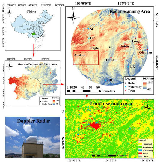
Figure 1.
Overview of study area and X-band radar location.
Radar is installed in Guiyang city (26°22′ N, 106°37′ E), China, and the radar antenna elevation is 1199 m. The scanning radius of the radar is 150 km, and the range of radiation from the selected radar position to the outside is approximately 100 km. The research area has an elevation of 402 m to 1949 m, with an average elevation of 1198 m. The terrain in the area is complicated and undulates greatly. Overall, the terrain is characterized by high elevation in the west and low elevation in the east, with obvious north-south longitudinal ridges and valleys. By selecting different land surfaces in the southwest portion of the radar scanning range to analyze the effects of atmospheric water vapor content changes, we find that vegetation and farmland surfaces are the main land surface types. The main cities and towns in the region are concentrated, while the rivers and lakes are scattered. For the verification of the effects of different land surfaces on atmospheric water vapor changes, we also selected some typical urban sites and water bodies at different elevations to evaluate regional land surface characteristics.
Due to the ascending topography and intense thermal changes on the underlying land surface, the atmospheric water vapor content in this region is subject to the complex thermal radiation of the low atmospheric boundary layer during circulation. Obvious thermal forcing and geodynamic lifting effects determine the unique regional climate and environmental characteristics of the low- and middle-latitude plateau; the water vapor above the plateau tends to change dramatically. Additionally, the region has a large population and is an important vulnerable environment and region of protected biodiversity in China that is very sensitive to climate change. In addition, there are few studies on water vapor changes and land surface conditions in this region due to various reasons, such as an underdeveloped economy and the great difficulties associated with research. Therefore, the atmospheric water vapor changes in this region have strong seasonal characteristics, and this periodic transformation and change in atmospheric water vapor are representative of global changes and are of high scientific value.
2.1.2. Random Sampling by Elevation
Sample points were randomly selected at different elevation intervals, and then the mean values of accumulated instantaneous reflectivity (IR) and the corresponding standard deviations (STD) for different elevations were obtained through Equations (1) and (2). After spatially matching the digital elevation model (DEM) data with accumulated IR data and the STD of the corresponding sample points in the time series, the relationship between atmospheric water vapor and terrain at different elevations was established. To explore the different effects of warm and cold seasons on atmospheric circulation, accumulated IR data from the same months were superimposed for analysis, and the changes in water vapor content that occur in different seasons were obtained. Equations (1) and (2) are expressed as follows:
where Z is the arithmetic mean of the IR values, is the daily IR value, μ is the average IR value of all days, and STD is the standard deviation, reflecting the dispersion of the data set.
2.1.3. Spatial Overlay and Clustering Analysis
For the analysis of land use data in the study area, two kinds of extraction techniques were used: regional and typical. The southwest region of the radar scanning range was taken for a regional analysis, and then different cities and towns or water bodies were selected for typical analysis and verification (Figure 1). Different land surface types and numbers were separated by spatial overlay and cluster analyses, and then urban impervious surfaces, large water bodies, vegetation coverage and other land use patches in the study area were extracted. Meanwhile, the spatial overlay of different land surfaces and IR data in the time series was carried out, and the spatial analysis between them was discussed.
Due to the great impact of different seasons on atmospheric water vapor content, the IR data were processed monthly and quarterly. After the monthly IR data were obtained, April to September was set as the warm season, while October of a given year to March of the next year was set as the cold season. Then, water vapor data representing the conditions above the land surface were established to obtain the monthly change trend under different land surface conditions. The STD was calculated by using the different IR data of each pixel position to discuss the stability of the change trend of the corresponding IR value in the time series and to complete the spatiotemporal analysis of the various categories.
2.1.4. Kernel Density Estimation
Kernel density estimation (KDE) is a nonparametric method that uses local information defined by windows (also called kernels) to estimate the densities of specified features at given locations in a study area. KDE is an important method used for mapping the spatial patterns of point events and has applications in ecology [24,25]. KDE over a two-dimensional space can be represented as follows [26]:
where f(x, y) is the estimated density value at location (x, y), n is the total number of event points under concern (e.g., disease cases), h is a measure of the window width and is called the kernel bandwidth (e.g., for a circular kernel, it is the radius of the circle), is the distance between the event point i and location (x, y), and K is a density function characterizing how the contribution of point i varies as a function of .
The representative normalized difference vegetation index (NDVI) was calculated to represent the warm season on 12 August 2019 and to represent the cold season on 19 March 2020. In the overlapping area of the satellite image and radar range, 100 random sample points were selected, each with corresponding NDVI and IR values. The changes in their distribution densities were established based on their correlations, and the effect of vegetation on water vapor variation was discussed. The KDE method was used to evaluate the relationship between the NDVI and IR. The density contour center is considered to be a place with a high probability of occurrence. When the NDVI increased at a certain stage, the enhancement effect on the density of the atmospheric water vapor distribution was obvious.
2.2. Doppler Radar Reflectivity and Different Land Surface Data
2.2.1. Doppler Radar Data
The radar data used in the study were obtained by an X-band Doppler bipolar weather radar (Figure 1 and Figure 2). The mode of the radar scanning is the plain position indicator (PPI), with a fixed angle of 0.5 degrees and a maximum threshold of 55 dBZ. The scanning period was 3 min, and the spatial resolution of the data is 150 m. The instantaneous reflectivity observation data of a single scan at 12:00 every day were selected as the observation values of that day, and the data mode of the instantaneous reflectivity (IR) of the radar was used for the analysis. There are 234 days of data from August 2017 to October 2019 used in this study. After screening the distorted data caused by mechanical faults or other reasons, 187 days of valid IR data with an approximately 100 km scanning range were selected as the research objects, including 117 days in the warm season and 70 days in the cold season.
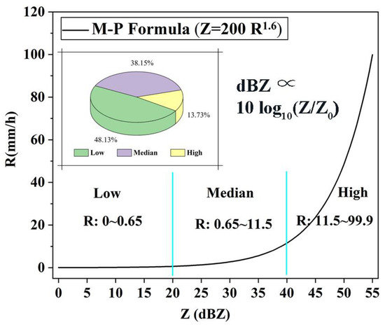
Figure 2.
Distribution characteristics of X-band radar data and Z–R relation curve.
The radar reflectivity values were converted into rain rates using the Marshall-Palmer (MP) formula [27], Z = 200 , and the reflectivity (Z) data are converted into instantaneous rain rates (R) [28]. Radar data were transformed into water vapor content parameters. Therefore, by utilizing the backward scattering characteristics of precipitable water and cloud droplets by Doppler weather radar, dynamic monitoring of atmospheric water vapor in weather systems with a high spatial-temporal accuracy can be established. The radar reflectivity data were divided into three intervals: low-, medium-, and high-range (LMH), which indicate 0–20, 20–40, and 40–55 dBZ, respectively. The change curve based on the M-P formula indicates the growth relationship of the water vapor content and radar reflectivity in these different intervals (Figure 2).
2.2.2. Land Surface Data
The land surface data used in this study include a digital elevation model (DEM), spatial vector data of different land use types, and red and near-infrared image data from Sentinel-2 satellites. The DEM represents topographic changes in the study area and describes the spatial distribution of different geomorphic factors, such as elevation, aspect and slope changes. Based on different land surface vector data, the distributions of different land use types were obtained; then, the other surface thermodynamic effects that remained after the terrain influence was excluded were discussed. Three kinds of surface vector data were selected with which to discuss the impacts of different land surface conditions: urban impervious surfaces, large surface water bodies, and vegetation coverage areas (Table 1).

Table 1.
Land surface data in the regional spatial distribution. DEM, digital elevation model; NDVI, normalized difference vegetation index.
In addition to the spatial vegetation coverage data, the normalized difference vegetation index (NDVI) was calculated by the red and near-infrared bands of Sentinel-2 images to judge the stabilization and regulation of the vegetation growth status on the weather and climate conditions. The NDVI was proposed in Tucker to assess the level of green vegetation and is arguably the most widely implemented remote sensing spectral index for monitoring Earth’s land surface. The NDVI was calculated by using the following equation [29]:
where NIR represents the near-infrared band digital number and R represents the red band digital number.
3. Results
3.1. Orographic Effects on the Variation of Atmospheric Water Vapor
The altitude in the study area varies greatly and can be classified into four stages, 400–500 m (S1), 600–1200 m (S2), 1300–1700 m (S3), and 1800–1900 m (S4), and the dynamic lifting effect of topography is obvious. The water vapor content increases with elevation from 600 m to 1200 m but decreases gradually after the elevation reaches 1200 m (Figure 3). The atmospheric water vapor content rises along with the elevation during atmospheric movement and goes through four main stages (Figure 3a), which are defined primarily by the amount of water vapor content accumulated and the stability of the state depending on the elevation. Stage S1 represents a relatively stable state with an average cumulative IR of 135.7 dBZ. The water vapor content changes briefly at this altitude stage, which is related to low-altitude topographic changes in the region. The average cumulative IR of stage S2 is 202.0 dBZ, which is 48.8% higher than that of S1 and shows a very good positive correlation. IR increases by 28.5% for each 100 m and reaches its highest point at 1200 m. At this time, the cumulative IR is 298.0 dBZ, the stability is the lowest, and the standard deviation reaches a peak value of 9.35. Stage S3 enters the height at which condensation descent of atmospheric water vapor occurs; the accumulated IR is in a stage of slow decrease, and the IR decreases by 1.9% for each 100 m increase on average, but the moisture content remains at a high level continuously, with an average accumulated IR of 268.1 dBZ, 32.7% higher than that of the previous stage. Finally, there is a sudden drop in the accumulated IR at stage S4; that at an altitude of 1800 m is 47.7% lower than that at the previous 1700 m, while the standard deviation at 1900 m is at its lowest value, 5.08, maintaining the most stable level of the whole altitude gradient.
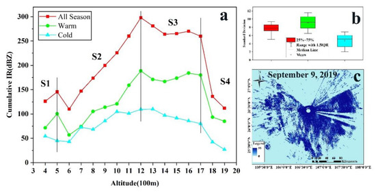
Figure 3.
Relationship between altitude and atmospheric water vapor content. (a) Variation in atmospheric water vapor content with altitude in different seasons, S1–4 are four stages according to the altitude, 400–500 m (S1), 600–1200 m (5S2), 1300–1700 m (S3), 1800–1900 m (S4); (b) standard deviations of the distributions of radar data in different seasons; (c) orographic effect on radar scanning range, taking 9 September 2019 as an example.
Variations to the stages in the warm season has a great influence on the change trend of the whole season. The cumulative average IR values of the different stages during the warm season, S1, S2, S3, and S4, account for 63.4%, 57.8%, 65.3%, and 72.0% of the total values throughout the season, respectively. The change trend during the cold season is relatively flat, and the distribution and change in atmospheric water vapor are relatively uniform during this time. The IR value remains at a low level for a long time and changes relatively slowly with increasing or decreasing altitude. The maximum IR value in the cold season occurs at an altitude of 1300 m. The changes and distributions of atmospheric water vapor in different seasons are basically in accordance with the rule that the water vapor content is affected by the topographic dynamic lift effect, but the range is quite different among different stages. As they are controlled by different monsoon conditions, there are obvious stability differences among the different seasons. The standard deviation range in the warm season is significantly larger than that in the cold season. The mean standard deviation in the warm season is 9.08, while that in the cold season is only 4.72 (Figure 3b). To illustrate the topographic effects on atmospheric water vapor distribution, a case study was conducted on 9 September 2019, when there were large amounts of precipitation and cloud droplet accumulation in the study region (Figure 3c). It can be clearly proven that the areas with low IR values in the south and east of the study area are also located at higher altitudes.
3.2. Water Vapor above Urban Surfaces in Different Seasons
IR values show obvious extreme cold- and warm-season trends (Figure 4). Changes in atmospheric water vapor in the warm season are affected by the southeast monsoon. The water vapor content increases rapidly during this season and maintains high-range values for months. In the cold season, affected by the southwest Indian Ocean monsoon and topography, a southwest quasi-static front is generated from November and December of a given year to January of the next year, and the atmospheric water vapor content continues to rise. For urban land surfaces, the average level of IR data varies among different seasons, with 29.5 dBZ in the warm season and 25.1 dBZ in the cold season, a maximum of 33.3 dBZ in August and a minimum of 20.3 dBZ in November. A seasonal analysis of atmospheric water vapor changes over the impervious urban surface at the beginning or end of different seasons shows that the distribution of water vapor in the cold season is more concentrated and slightly less than that in the warm season. The distribution of water vapor is most extreme in August and November, and these months are controlled by different monsoon conditions. The distribution during the warm season is more dispersed and has a higher mean value than that during the cold season. The fluctuation range during the cold season is limited and stable.
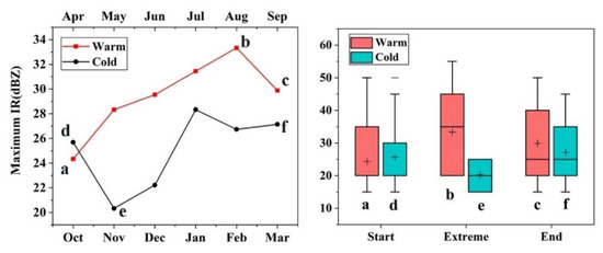
Figure 4.
Monthly variation and extreme trends of instantaneous reflectivity (IR) of urban impervious surface (a and d represent the beginning of warm season and cold season, b and e are extreme cases, c and f are the end of season).
The variation in atmospheric water vapor in towns at different elevations (ELs) is roughly in accordance with the law of water vapor transmission over impervious surfaces in the region. However, different geographical locations and altitudes have some minor effects on water vapor changes. High towns (HTs) include Longli (EL: 1089 m), Pingba (EL: 1268 m), and Anshun (EL: 1358 m), and the water vapor contents above HTs are basically higher than those in the region as a whole (Figure 5). The climate process of extreme atmospheric water transmission is more obvious in Anshun in July and August, as there is more atmospheric water present in the warm season. The monthly IR values in July and August are 14.3% and 10.7% higher, respectively, in the HTs than those in the whole region. Low towns (LTs) include Guiding (EL: 998 m), Qiannan (EL: 786 m), and Huishui (EL: 967 m), and the water vapor distributions at these low elevation towns are slightly lower than those of regional urban surfaces. The IR values of HTs in the warm and cold seasons are 30.5 dBZ and 26.2 dBZ, respectively, while those of LTs in the warm and cold seasons are 28.8 dBZ and 24.6 dBZ, respectively. The IR values of urban impervious surfaces measured after rising in elevation increase by 5.9% and 6.5% in the warm and cold seasons, respectively.
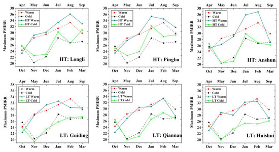
Figure 5.
Change trends of water vapor in typical towns at different altitudes. The solid line for high town (HT)/low town (LT) is a typical town, and the dotted line represents the average of urban region.
3.3. Spatial and Seasonal Variations in Water Vapor over Water Bodies
Compared with the previous month, the change trend of each month studied is relatively different. The change rate of water vapor content in the warm season has a highest change rate of 7.3% and a lowest change rate of −12.5% (Figure 6). The highest water vapor content in the cold season is 23.1% higher than that in the previous season, while the lowest is −12.9% less than that in the previous season. In the warm season, the evaporation of water bodies is intensified due to the increase in temperature, which weakens the extreme water vapor convection over the water surfaces. In the cold season, the atmospheric condition is affected by the southwest Indian Ocean monsoon, and the water vapor present over large water bodies causes the regional convection to weaken. The atmospheric conditions controlled by quasi-stationary fronts over the region bring about discontinuous rainy weather, so the change trend of the water vapor content is unpredictable. There is substantial uncertainty about the state of atmospheric water as it is affected by fronts. A large water body surface has a weak influence on atmospheric water vapor over that surface, which makes the movement and change process of water vapor in the region more moderate than those above other surface types, but the variation trends are also completely different between the warm and cold seasons.
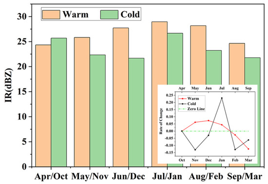
Figure 6.
Monthly IR values and change rates in the warm and cold seasons.
The influence of altitude on water vapor contents above large water bodies cannot be ignored. There are still some differences in the average IR values of large water body areas between high altitudes and low altitudes. The atmospheric water contents in high-altitude areas are slightly higher than those in low-altitude areas (Figure 7), but the transport law of water from water bodies to atmospheric water is also obvious. For high-elevation water bodies (HWs), such as the Liuchong River (EL: 951 m) and Sancha River (EL: 959 m), the changes in atmospheric water have certain fluctuations compared with that of the water bodies of the region as a whole. For low-elevation water bodies (LWs), such as the Lianjiang River (EL: 538 m) and Caodu River (EL: 640 m), the change trends are relatively stable.
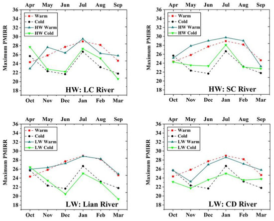
Figure 7.
Monthly IR values and change rates in the warm and cold seasons. The solid line for high-elevation water bodies (HWs)/low-elevation water bodies (LWs) is one water body, and the dotted line represents the average of all water bodies.
3.4. Vegetation Distribution Influences on the above Water Vapor Content
The NDVI ranges from 0 to 0.81 in the warm season, and the average IR is 109.9 dBZ. Due to the weakening of vegetation in the cold season, the average distribution of the NDVI is low in this season (the maximum value is only 0.70), and the average IR is 60.65 dBZ, which is 44.8% lower than that in the warm season. The results show that when the NDVI value increases from 0.6 to 0.7, a contour center is formed (Figure 8c,d) that is more obvious in the warm season, and a strong probability density center is formed that is much weaker in the cold season (Figure 8). This indicates that the vegetation coverage of the land surface greatly improves the transformation conditions of regional atmospheric water, keeping the water vapor values at relatively wet levels. This enhancement is evident in the warm season but is significantly reduced in the cold season due to the weakening of vegetation. Vegetation coverage and plant growth affect the movement and transformation of water vapor in the lower atmosphere, causing the moisture content in the atmosphere to be more abundant for a long time but also inhibiting the occurrence of extreme weather conditions.
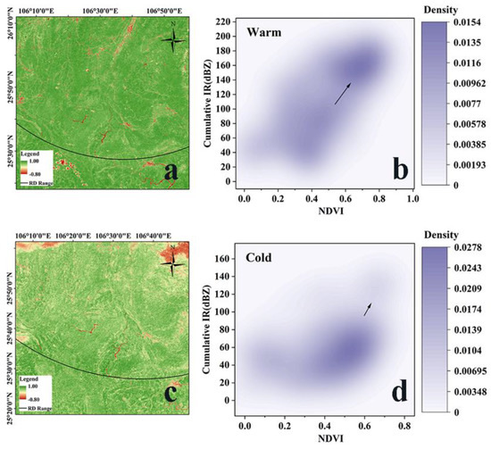
Figure 8.
Distributions of the NDVI and KDE values in different seasons in the scanning region. (a) The NDVI on August 12, 2019, obtained from Sentinel satellite data; (b) KDE diagram generated from the NDVI and cumulative radar data in 2019; (c) the NDVI on 19 March 2020; (d) KDE diagram generated from the NDVI and cumulative radar data in 2020.
3.5. Comparison of Atmospheric Water Vapor Contents over the Three Typical Land Cover Types
The movement and transformation processes of atmospheric water vapor are affected by the thermodynamic conditions of different land surfaces. Upward vertical convection of the lower atmosphere can be enhanced or suppressed by the land surface, resulting in changes in the water vapor content over the surface. The IR values of different surfaces are mainly concentrated in the low range, which indicates low atmospheric water contents (Figure 9). The probabilities of low-range values over typical surfaces such as urban towns, water bodies, and vegetation are 49.7%, 48.7%, and 46.0%, respectively, showing a slight downward trend. The median-range probabilities of the humid atmosphere are 31.6%, 38.5%, and 44.4% for the same three surface types, respectively. Compared with urban surface types, large water bodies and vegetation coverage areas have good regulation and enhancement effects on their overlying water vapor contents. This means that, due to the impacts of water bodies and vegetated surfaces, there are always high atmospheric humidity values above these surfaces. When concentrated in the high range, the probability of water vapor content values above urban surfaces is higher than those of other, natural land surface types, and the probabilities of high-range water vapor contents above land surface such as towns, water bodies and vegetation are 18.7%, 12.8%, and 9.6%, respectively. This indicates that the urban land type changes the impervious underlying surfaces and has different thermodynamic effects from the adjacent surfaces; this difference aggravates the occurrence of extreme climatic events during the processes of atmospheric water changes. This phenomenon is also clearly different from the processes above vegetation coverage and water body surfaces. Generally, urban impervious surfaces make atmospheric water vapor more extreme, and dry conditions of low-range values and convection weather of high-range values become more obvious. The atmospheric water vapor distributions over large water body surfaces are more balanced. Over typical vegetation coverage, the water vapor probability can be reduced in both the low and high ranges, maintaining the water vapor status in the median range over long durations.
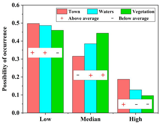
Figure 9.
Probability of occurrence of water vapor in different ranges.
The distributions of the IR data representing different land surface types in the cold and warm seasons show obvious differences (Figure 10). For the urban impervious surface type, the probability of extreme climate events occurring under the process of water vapor movement and changes in the high-reflectivity range is 23.1% under the influence of the Western Pacific warm season monsoon. In the weather system controlled by the southwest quasistatic stop front caused by the Indian Ocean monsoon, the probability of extreme climate events in the cold season drops to 11.4%. Compared with that of the warm season, the equilibrium effect of the atmospheric water vapor distribution is slightly different in the cold season. Changes in atmospheric circulation and the contraction of geothermal dynamic conditions in the cold season make atmospheric water vapor more concentrated at the low and median levels. The distribution of water vapor is more concentrated in the cold season than in the warm season, in which it increases by 8.1%. The water vapor content over vegetation coverage areas is mainly distributed at the median range, and the seasonal change in this range is small. The extreme processes in the high range are obviously reduced. Under the combined actions of monsoon circulation and vegetation, the occurrence probability of high-range values in the cold season is only 33.4% of that in the warm season.
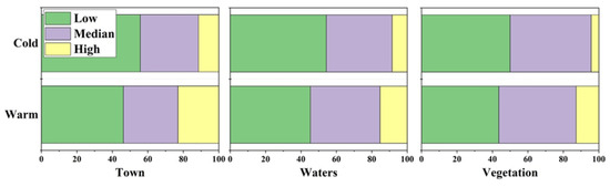
Figure 10.
Seasonal distributions of the probability of occurrence of the water vapor range on different surfaces.
4. Discussion
4.1. Elevation Is A Leading Role Which Influences the Content and Distribution of Atmospheric Water Vapor
The elevation of terrain forces atmospheric water vapor to rise during its movement. Topographic controls on hydrometeorology have been observed before, and elevation has been observed as imparting the primary control [30]. In this study (Figure 3), due to the limited topography at S1, the water vapor content change is relatively weakly affected by the topography, and the water vapor climbs rapidly under the influence of circulation dynamics. Therefore, S1 imparts a small fluctuation in the water vapor content, but the water vapor content always remains in the low range. The results show that there is a very good positive correlation between the accumulated IR values of S2 and the altitude of 600 m–1200 m. Dynamic cooling of atmospheric water gradually occurs during the climbing process, and the atmospheric water then condenses into precipitable water and cloud droplets with larger backscattering coefficients; thus, the variation in atmospheric water begins to enter an unstable and violent period with increasing altitude. After the water vapor content reaches its peak value at 1200 m, the change in the water vapor content enters stage 3. During S3, the altitude is between 1300 m and 1700 m. Due to the gradual loss of the ascending power of atmospheric water, the water vapor is converted to land surface water, resulting in topographic rainfall, which causes the composition of water vapor in the atmosphere and the IR of the elevation to gradually decrease. Over 1800 m, atmospheric water re-enters the final stage of stability. At this time, it is at high altitudes from 1800 m to 1900 m. During this stage, the obstruction effects of complex orography and elevation are weakened. The movement of the atmosphere above the mountains is relatively smooth, and atmospheric water passes through quickly. At this time, it is difficult to form large-scale water vapor accumulation.
Altitude is an important factor of topography, and the relationship between altitude and precipitable water has always been the focus of topographic precipitation research [31,32,33]. Due to the topographic effect, precipitable water and cloud droplets in complex terrain areas increase with increasing altitude. In the southern Himalayas, precipitation also has similar characteristics. Precipitation increases with elevation but decreases with elevation after the elevation exceeds 2500 m [34]. Atmospheric water vapor gradually condenses and forms a more stable rainfall area. The spatial distribution and evolution of precipitation around terrain is closely related to the height, scale, shape, slope direction, and gradient of the terrain [35,36]. Precipitation increases with increasing altitude. After reaching a certain height, precipitation no longer increases with altitude. Conversely, precipitation then decreases sharply and tends to stabilize. The formation and evolution of precipitable water and cloud droplets are affected by terrain through a series of physical processes, such as cloud microphysics, dynamics, and thermodynamics.
4.2. Urban Site Effect Influences the Water Vapor in the Atmosphere
Different cities and towns have different impacts on climate. Urban heat islands (UHIs) are phenomena resulting from climate change and urbanization [37,38] and are described as urban areas with significantly warmer temperatures than those of the surrounding rural areas. Urban agglomerations with large-scale impervious surfaces have not been found to change a wide range of atmospheric climatic conditions but mainly consist of small villages and towns wherein human activities occur, so there is no obvious UHI effect attributed to these urban agglomerations. However, small urban impervious surfaces can still develop to affect extreme climate conditions (Figure 4). This rule is also related to different altitudes, and increased city sizes are also obvious to this effect (Figure 5). For example, as a high town (HT), Anshun has an obvious and extreme UHI effect because Anshun has a relatively large urban scale and is in a high-altitude position. This shows that urban scale and altitude are both important factors affecting the change in water vapor content over the land surface. For the other towns, the extreme trends are not as obvious due to their small scales.
The UHI phenomenon is generally considered to be caused by a reduction in latent heat flux and an increase in sensible heat in urban areas as vegetated and evaporating soil surfaces are replaced by relatively impervious, low-albedo paving and building materials. Urban heating and the formation of UHIs reflect a broad suite of important land surface changes impacting ecosystem functions, local weather conditions, and possibly climate conditions [39]. Human activities and urban development have led to regional warming. Evapotranspiration due to temperature change has direct relations to increases or decreases in PWV and rainfall, with subsequent weather changes and increased disaster frequencies posing threats to the natural environment and to the property of humans. The detection of meteorological changes requires lengthy monitoring. Following past studies of the meteorology of Taiwan [40], in short, the development of urban areas has changed the natural characteristics of the underlying surfaces, resulting in a substantial increase in the impervious area and decreases in the vegetation and water areas, all of which change the heat capacities of the underlying surfaces. At the same time, due to urban functions, more industrial heat is generated, which more easily absorbs solar radiation, forming a heat island effect. Thus, thermal effects of UHIs that are fundamentally different from those of other land surface types are formed.
4.3. Water Vapor over Water Body Maintains the Moderate Content
The presence of a water body causes the distribution range of the water vapor content above its surface to change, and the proportions of each part (LMH) are more balanced than those above other land surface types. Although they are affected by seasonal atmospheric circulation, the trends vary dramatically (Figure 6). The impact of water bodies on atmospheric water vapor is mainly caused by the difference between the thermodynamic conditions above the water surface and those on the land surface. Water bodies increase local evaporation and maintain moderate water vapor contents in the atmosphere. Regulating local water vapor conditions and buffering the condensation and transformation of water vapor are also balanced effects. The reflectivity and net radiation values vary greatly with the physical properties of water and land surfaces. Water surfaces cause the net radiation to be significantly higher than that of the land surface. The difference in net radiation between a water surface and land surface affects the change in the near-air temperature. Due to the influence of the water body temperature, the range of temperatures above and around a water body is smaller than that of the land surface. Generally, the water vapor content above a water body is higher than that above the surrounding land, and the monthly and annual average absolute humidity and relative humidity values increase. For large water bodies, evaporation increases the water vapor content in the atmosphere, thus increasing the amount of water available for precipitation. In addition, water surface evaporation accounts for a very small proportion of the total precipitation.
Water bodies have the ability to adjust their surrounding microclimates [41]. Water vaporization allows the ambient atmosphere to absorb latent heat and significantly decreases the ambient air temperature; thus, water bodies (including lakes and rivers) provide important local climate-regulating services [42]. Due to the climatic conditions over a water body, atmospheric water vapor does not easily condense, so the occurrence of extreme situations decreases. The IR range over a water body also generally reflects the process from the accumulation to the transfer of evaporated water vapor under the influence of factors such as wind and topography. Although different water bodies have distinct influences on the above water vapor, select types of water bodies often exist in special topographies, such as canyons, which have great influences on local water vapor variation (maybe much greater than the influences of the water bodies themselves on the above atmospheric water movement). In the Yunnan–Guizhou Plateau area, the warm season is mainly controlled by the West Pacific monsoon. The strong southeast monsoon brings more than 60% of the total amount of annual water vapor in a concentrated time period. The atmospheric water vapor brought to the plateau begins to change dramatically under the influence of the land surface. In the cold season, due to the existence of the Kunming quasistatic front, the eastern wind current near the ground surface along the terrain in the eastern region of the Yunnan-Guizhou Plateau slowly lifts due to terrain obstruction. Under the action of high-level westerly winds, the upward atmospheric flow is diverted to the east, thus forming a relatively stable local secondary circulation pattern in the near-ground layer and gradually forming long-term atmospheric water vapor accumulation after November. This results in continuous water vapor transformation and is the root cause of seasonal changes in water vapor.
4.4. Mutual Feedback between Vegetation and Water Vapor Content Is Obvious
Vegetation coverage can significantly regulate the moisture content and increase the humidity of atmospheric air. The cooling effect of vegetation has been widely documented [43,44,45,46]. Vegetation cools the environment through the moderation of the land surface temperature by shading the land surface from direct sunlight, intercepting solar radiation, and consequently altering heat fluxes [47,48,49]. Vegetation also cools the air through the process of evapotranspiration [50,51,52]. When vegetation growth is weakened, this effect is also greatly weakened (Figure 10). Vegetation, which plays a significant role in the exchanges of energy, water, and carbon between the land surface and atmosphere, is the main component of terrestrial ecosystems [53]. The response of vegetation coverage to the climate is a complicated process, and vegetation is also one of the main factors regulating water vapor content changes in this area of complex terrain. With good vegetation growth and high NDVI values, the IR values are maintained in the median range for a long time. Vegetation coverage not only changes the local temperature and energy budget but also affects local precipitation and the water cycle by changing circulation.
The vegetation canopy is a major contributor to cooling and moderating microclimatic environments [54,55]. With an increase in vegetation coverage on the underlying surface, transpiration is enhanced, and atmospheric water vapor increases over the area. In addition, ground friction increases due to an increase in vegetation coverage, resulting in atmospheric convergence and upward movement. Therefore, an increase in vegetation coverage accelerates the local water cycle. In areas with good vegetation development in the warm season, the processes of radiation balance and water balance can be affected by changing surface properties such as surface albedo, roughness, and soil moisture. Finally, the processes of regional precipitation, the circulation situation, atmospheric temperature, humidity, and other climate changes can become gentler with an increase in vegetation, thus stabilizing the climate. However, obtaining detailed and accurate quantifications of vegetation canopy structures (particularly shading resulting from canopy cover) and the effect of vegetation on cooling are still challenging, even when combined with micrometeorological observations [56].
5. Conclusions
In this work, based on the microwave characteristics of water vapor in the atmosphere, precipitable water and cloud droplets under weather systems were dynamically monitored in complex terrain and over different land surfaces using Doppler radar. The research shows that the water vapor content increases with elevation from 600 m to 1200 m, showing a good positive correlation. The atmospheric water vapor content then decreases gradually with increasing elevation after 1200 m and decreases significantly after 1700 m. The IR values in the impervious areas show obvious extreme seasonal variations between the cold and warm seasons. Water bodies have a slight influence on the change in water vapor over the atmosphere, causing the movement and variation processes of atmospheric water vapor in the region to be gentler than those above other surface types. Vegetation coverage and plant growth conditions affect the movement and transformation of atmospheric water vapor in the low atmosphere, causing the moisture content in the atmosphere to be abundant for a long time but inhibiting the occurrence of extreme weather conditions. This study provides the distribution and transformation rules of atmospheric water vapor in areas of complex terrain and quantitatively analyzes the relationships between different land surfaces and atmospheric water vapor by a high spatial-temporal method, improving our understanding of the law of atmospheric movement of different land surface conditions in a complex terrain area.
Author Contributions
Conceptualization, H.L. and S.Y.; methodology, J.Z.; software, J.Z.; validation, M.C., X.R. and Y.L.; formal analysis, C.L.; investigation, H.L.; resources, Y.L.; data curation, H.L.; writing—original draft preparation, J.Z.; writing—review and editing, H.L.; visualization, S.Y.; supervision, M.C.; project administration, Y.L.; funding acquisition, H.L. All authors have read and agreed to the published version of the manuscript.
Funding
The authors thank the National Natural Science Foundation of China (Grant Nos. U1812401, 41801334), the Open Research Fund Program of State key Laboratory of Hydroscience and Engineering (sklhse-2021-A-04), the Opening Fund of State Key Laboratory of Geohazard Prevention and Geoenvironment Protection (Chengdu University of Technology, SKLGP2020K005), the Fundamental Research Funds for the Central Universities (2017NT11).
Institutional Review Board Statement
Not applicable.
Informed Consent Statement
Not applicable.
Data Availability Statement
Data available on request.
Acknowledgments
Authors wish to thank my colleagues for help in collecting experimental data.
Conflicts of Interest
The authors declare no conflict of interest.
References
- Cheruy, F.; Ducharne, A.; Hourdin, F.; Musat, I.; Vignon, É.; Gastineau, G.; Bastrikov, V.; Vuichard, N.; Diallo, B.; Dufresne, J.L.; et al. Improved Near-Surface Continental Climate in IPSL-CM6A-LR by Combined Evolutions of Atmospheric and Land Surface Physics. J. Adv. Model. Earth Syst. 2020, 12, e2019MS002005. [Google Scholar] [CrossRef]
- IPCC. Summary for policymakers. In Climate Change 2013: The Physical Science Basis; Stocker, T., Qin, D., Platter, G.-K., Eds.; Cambridge University Press: Cambridge, UK, 2013; pp. 1–29. [Google Scholar]
- Huang, H.-Y.; Margulis, S.A. On the impact of surface heterogeneity on a realistic convective boundary layer. Water Resour. Res. 2009, 45. [Google Scholar] [CrossRef]
- Avissar, R.; Schmidt, T. An evaluation of the scale at which ground-surface heat flux patchiness affects the con-vective boundary layer using large-eddy simulations. J. Atmos. Sci. 1998, 55, 2666–2689. [Google Scholar] [CrossRef]
- Musa, T.; Amir, S.; Othman, R.; Ses, S.; Omar, K.; Abdullah, K.; Lim, S.; Rizos, C. GPS meteorology in a low-latitude region: Remote sensing of atmospheric water vapor over the Malaysian Peninsula. J. Atmos. Sol.-Terr. Phys. 2011, 73, 2410–2422. [Google Scholar] [CrossRef]
- Tan, Z.; Fang, J.; Wu, R. Ekman Boundary Layer Dynamic Theories. Acta Meteorol. Sin. 2005, 63, 543–555. [Google Scholar]
- Liu, S.; Shao, Y.; Kunoth, A.; Simmer, C. Impact of surface-heterogeneity on atmosphere and land-surface interactions. Environ. Model. Softw. 2017, 88, 35–47. [Google Scholar] [CrossRef]
- Smith, R.B. The Influence of Mountains on the Atmosphere. Adv. Geophys. 1979, 21, 87–230. [Google Scholar] [CrossRef]
- Held, I.M.; Ting, M.; Wang, H. Northern winter stationary waves: Theory and modeling. J. Clim. 2002, 15, 2125–2144. [Google Scholar] [CrossRef]
- Jin, S.; Li, Z.; Cho, J. Integrated Water Vapor Field and Multiscale Variations over China from GPS Measurements. J. Appl. Meteorol. Clim. 2008, 47, 3008–3015. [Google Scholar] [CrossRef]
- Santer, B.D.; Mears, C.; Wentz, F.J.; Taylor, K.E.; Gleckler, P.J.; Wigley, T.M.L.; Barnett, T.P.; Boyle, J.S.; Bruggemann, W.; Gillett, N.P.; et al. Identification of human-induced changes in atmospheric moisture content. Proc. Natl. Acad. Sci. USA 2007, 104, 15248–15253. [Google Scholar] [CrossRef] [PubMed]
- Gedney, N.; Cox, P.M.; Betts, R.A.; Boucher, O.; Huntingford, C.; Stott, P.A. Detection of a direct carbon dioxide effect in continental river runoff records. Nat. Cell Biol. 2006, 439, 835–838. [Google Scholar] [CrossRef] [PubMed]
- Zhang, X.; Zwiers, F.W.; Hegerl, G.C.; Lambert, F.H.; Gillett, N.P.; Solomon, S.; Stott, P.A.; Nozawa, T. Detection of human influence on twentieth-century precipitation trends. Nat. Cell Biol. 2007, 448, 461–465. [Google Scholar] [CrossRef] [PubMed]
- Willett, K.M.; Gillett, N.P.; Jones, P.D.; Thorne, P.W. Attribution of observed surface humidity changes to human influence. Nat. Cell Biol. 2007, 449, 710–712. [Google Scholar] [CrossRef]
- Tianbao, Z.; Kai, T.; Zhongwei, Y. Advances of Atmospheric Water Vapor Change and Its Feedback Effect. Adv. Clim. Chang. Res. 2013, 9, 79–88. [Google Scholar]
- Woodhouse, I.H. Introduction to Microwave Remote Sensing; CRC Press: Boca Raton, FL, USA, 2017. [Google Scholar]
- Yeh, T.-K.; Chan, S.-L.; Shih, H.-C.; Su, K.-C. Ground-based GPS remote sensing for precipitable water vapor: A case study of the heat-island effect in Taipei. Terr. Atmos. Ocean. Sci. 2019, 30. [Google Scholar] [CrossRef]
- Guerova, G.; Brockmann, E.; Quiby, J.; Schubiger, F.; Matzler, C. Validation of NWP Mesoscale Models with Swiss GPS Network AGNES. J. Appl. Meteorol. 2003, 42, 141–150. [Google Scholar] [CrossRef]
- Bevis, M.; Businger, S.; Herring, T.A.; Rocken, C.; Anthes, R.A.; Ware, R.H. GPS meteorology: Remote sensing of atmospheric water vapor using the global positioning system. J. Geophys. Res. Space Phys. 1992, 97, 15787–15801. [Google Scholar] [CrossRef]
- Emanuel, K.; Raymond, D.; Betts, A.; Bosart, L.; Bretherton, C.; Droegemeier, K.; Farrell, B.; Fritsch, J.M.; Houze, R.; Le Mone, M.; et al. Report of the First Prospectus Development Team of the U.S. Weather Research Program to NOAA and the NSF. Bull. Am. Meteorol. Soc. 1995, 76, 1194–1208. [Google Scholar]
- Nanding, N.; Rico-Ramirez, M.A.; Han, D. Comparison of different radar-raingauge rainfall merging techniques. J. Hydroinform. 2015, 17, 422–445. [Google Scholar] [CrossRef]
- Zou, J.; Liu, H. Distribution of water vapor content and its seasonal variation over the mainland China. Adv. Atmos. Sci. 1986, 3, 385–396. [Google Scholar] [CrossRef]
- Zhai, P.; Eskridge, R.E. Atmospheric Water Vapor over China. J. Clim. 1997, 10, 2643–2652. [Google Scholar] [CrossRef]
- Worton, B.J. Kernel Methods for Estimating the Utilization Distribution in Home-Range Studies. Ecology 1989, 70, 164–168. [Google Scholar] [CrossRef]
- Brunsdon, C. Estimating probability surfaces for geographical point data: An adaptive kernel algorithm. Comput. Geosci. 1995, 21, 877–894. [Google Scholar] [CrossRef]
- Silverman, B.W. Density Estimation for Statistics and Data Analysis; Chapman & Hall/CRC: Boca Raton, FL, USA, 1986. [Google Scholar]
- Marshall, J.S.; Hitschfeld, W.; Gunn, K.L.S. Advances in Radar Weather. Adv. Geophys. 1955, 2, 1–56. [Google Scholar]
- Delobbe, L.; Watlet, A.; Wilfert, S.; Van Camp, M. Exploring the use of underground gravity monitoring to evaluate radar estimates of heavy rainfall. Hydrol. Earth Syst. Sci. 2019, 23, 93–105. [Google Scholar] [CrossRef]
- Tucker, C.J. Red and photographic infrared linear combinations for monitoring vegetation. Remote Sens. Environ. 1979, 8, 127–150. [Google Scholar] [CrossRef]
- Vivoni, E.R.; Gutiérrez-Jurado, H.A.; Aragón, C.A.; Méndez-Barroso, L.A.; Rinehart, A.J.; Wyckoff, R.L.; Rodríguez, J.C.; Watts, C.J.; Bolten, J.D.; Lakshmi, V.; et al. Variation of hydrometeorological conditions along a topo-graphic transect in northwestern Mexico during the North American monsoon. J. Clim. 2007, 20, 1792–1809. [Google Scholar] [CrossRef]
- Basist, A.; Bell, G.D.; Meentemeyer, V. Statistical Relationships between Topography and Precipitation Patterns. J. Clim. 1994, 7, 1305–1315. [Google Scholar] [CrossRef]
- Alijani, B. Effect of the Zagros Mountains on the spatial distribution of precipitation. J. Mt. Sci. 2008, 5, 218–231. [Google Scholar] [CrossRef]
- Al-Ahmadi, K.; Al-Ahmadi, S. Rainfall-altitude relationship in Saudi Arabia. Adv. Meteorol. 2013, 2013, 363029. [Google Scholar] [CrossRef]
- Salerno, F.; Guyennon, N.; Thakuri, S.; Viviano, G.; Romano, E.; Vuillermoz, E.; Cristofanelli, P.; Stocchi, P.; Agrillo, G.; Ma, Y.; et al. Weak precipitation, warm winters and springs impact glaciers of south slopes of Mt. Everest (central Himalaya) in the last 2 decades (1994–2013). Cryosphere 2015, 9, 1229–1247. [Google Scholar] [CrossRef]
- Roe, G.H. Orographic Precipitation. Annu. Rev. Earth Planet. Sci. 2005, 33, 645–671. [Google Scholar] [CrossRef]
- Kumari, M.; Singh, C.K.; Bakimchandra, O.; Basistha, A. DEM-based delineation for improving geostatistical in-terpolation of rainfall in mountainous region of Central Himalayas, India. Theor. Appl. Climatol. 2017, 130, 51–58. [Google Scholar] [CrossRef]
- Bowler, D.E.; Buyung-Ali, L.; Knight, T.M.; Pullin, A.S. Urban greening to cool towns and cities: A systematic review of the empirical evidence. Landsc. Urban Plan. 2010, 97, 147–155. [Google Scholar] [CrossRef]
- Kong, F.; Yan, W.; Zheng, G.; Yin, H.; Cavan, G.; Zhan, W.; Zhang, N.; Cheng, L. Retrieval of three-dimensional tree canopy and shade using terrestrial laser scanning (TLS) data to analyze the cooling effect of vegetation. Agric. For. Meteorol. 2016, 217, 22–34. [Google Scholar] [CrossRef]
- Imhoff, M.L.; Zhang, P.; Wolfe, R.E.; Bounoua, L. Remote sensing of the urban heat island effect across biomes in the continental USA. Remote. Sens. Environ. 2010, 114, 504–513. [Google Scholar] [CrossRef]
- Yeh, T.-C.; Liao, C.-S.; Chen, T.-C.; Shih, Y.-T.; Huang, J.-C.; Zehetner, F.; Hein, T. Differences in N loading affect DOM dynamics during typhoon events in a forested mountainous catchment. Sci. Total Environ. 2018, 633, 81–92. [Google Scholar] [CrossRef]
- Albdour, M.S.; Baranyai, B. Water body effect on microclimate in summertime: A case study from Pécs. Pollack Period. 2019, 14, 131–140. [Google Scholar] [CrossRef]
- Amani-Beni, M.; Zhang, B.; Xie, G.-D.; Xu, J. Impact of urban park’s tree, grass and waterbody on microclimate in hot summer days: A case study of Olympic Park in Beijing, China. Urban For. Urban Green. 2018, 32, 1–6. [Google Scholar] [CrossRef]
- Dimoudi, A.; Nikolopoulou, M. Vegetation in the urban environment: Microclimatic analysis and benefits. Energy Build. 2003, 35, 69–76. [Google Scholar] [CrossRef]
- Yu, C.; Hien, W.N. Thermal benefits of city parks. Energy Build. 2006, 38, 105–120. [Google Scholar] [CrossRef]
- Giridharan, R.; Lau, S.S.Y.; Ganesan, S.; Givoni, B. Lowering the outdoor temperature in high-rise high-density residen-tial developments of coastal Hong Kong: The vegetation influence. Build. Environ. 2008, 43, 1583–1595. [Google Scholar] [CrossRef]
- Fahmy, M.; Sharples, S.; Yahiya, M. LAI based trees selection for mid latitude urban develop-ments: A microclimatic study in Cairo, Egypt. Build. Environ. 2010, 45, 345–357. [Google Scholar] [CrossRef]
- Simpson, J.R. Improved estimates of tree-shade effects on residential energy use. Energy Build. 2002, 34, 1067–1076. [Google Scholar] [CrossRef]
- Tsiros, I.X. Assessment and energy implications of street air temperature cooling by shade tress in Athens (Greece) under extremely hot weather conditions. Renew. Energy 2010, 35, 1866–1869. [Google Scholar] [CrossRef]
- Lindberg, F.; Grimmond, S. The influence of vegetation and building morphology on shadow patterns and mean radiant temperatures in urban areas: Model development and evaluation. Theor. Appl. Climatol. 2011, 105, 311–323. [Google Scholar] [CrossRef]
- Akbari, H.; Konopacki, S. Energy effects of heat-island reduction strategies in Toronto, Canada. Energy 2004, 29, 191–210. [Google Scholar] [CrossRef]
- Shashua-Bar, L.; Pearlmutter, D.; Erell, E. The cooling efficiency of urban landscape strategies in a hot dry climate. Landsc. Urban Plan. 2009, 92, 179–186. [Google Scholar] [CrossRef]
- Zhao, L.; Lee, X.; Smith, R.B.; Oleson, K.W. Strong contributions of local background climate to urban heat islands. Nat. Cell Biol. 2014, 511, 216–219. [Google Scholar] [CrossRef]
- De Jong, R.; de Bruin, S.; de Wit, A.; Schaepman, M.E.; Dent, D.L. Analysis of monotonic greening and browning trends from global NDVI time-series. Remote Sens. Environ. 2011, 115, 692–702. [Google Scholar] [CrossRef]
- Lowman, M.D.; Wittman, P.K. Forest canopies: Methods, Hypotheses, and Future Directions. Annu. Rev. Ecol. Syst. 1996, 27, 55–81. [Google Scholar] [CrossRef]
- Jupp, D.L.; Culvenor, D.S.; Lovell, J.L.; Newnham, G.J.; Strahler, A.H.; Woodcock, C.E. Estimating forest LAI pro-files and structural parameters using a ground-based laser called ‘Echidna®. Tree Physiol. 2009, 29, 171–181. [Google Scholar] [CrossRef] [PubMed]
- Tooke, T.R.; Coops, N.C.; Voogt, J.A.; Meitner, M.J. Tree structure influences on roof-top-received solar radiation. Landsc. Urban Plan. 2011, 102, 73–81. [Google Scholar] [CrossRef]
Publisher’s Note: MDPI stays neutral with regard to jurisdictional claims in published maps and institutional affiliations. |
© 2021 by the authors. Licensee MDPI, Basel, Switzerland. This article is an open access article distributed under the terms and conditions of the Creative Commons Attribution (CC BY) license (https://creativecommons.org/licenses/by/4.0/).