Article

The Impact of Aerosols on Satellite Radiance Data Assimilation Using NCEP Global Data Assimilation System

1
Atmospheric Sciences Research Center, University at Albany, Albany, NY 12203, USA
2
Joint Center for Satellite Data Assimilation, Boulder, CO 80301, USA
3
NOAA/NESDIS Center for Satellite Applications and Research, College Park, MD 20740, USA
4
I.M.Systems Group at NCEP/NWS/EMC, College Park, MD 20740, USA
5
I.M.Systems Group at NOAA/NESDIS/STAR, College Park, MD 20740, USA
6
NOAA/NWS National Centers for Environmental Prediction, College Park, MD 20740, USA
*
Authors to whom correspondence should be addressed.
Atmosphere 2021, 12(4), 432; https://doi.org/10.3390/atmos12040432
Submission received: 12 March 2021 / Revised: 24 March 2021 / Accepted: 24 March 2021 / Published: 28 March 2021
(This article belongs to the Special Issue Radiative Transfer in the Earth Atmosphere)

Abstract

:
Aerosol radiative effects have been studied extensively by climate and weather research communities. However, aerosol impacts on radiance in the context of data assimilation (DA) have received little research attention. In this study, we investigated the aerosol impacts on the assimilation of satellite radiances by incorporating time-varying three-dimensional aerosol distributions into the radiance observation operator. A series of DA experiments was conducted for August 2017. We assessed the aerosol impacts on the simulated brightness temperatures (BTs), bias correction and quality control (QC) algorithms for the assimilated infrared sensors, and analyzed temperature fields. We found that taking the aerosols into account reduces simulated BT in thermal window channels (8 to 13 μm) by up to 4 K over dust-dominant regions. The cooler simulated BTs result in more positive first-guess departures, produce more negative biases, and alter the QC checks about 20%/40% of total/assimilated observations at the wavelength of 10.39 μm. As a result, assimilating aerosol-affected BTs produces a warmer analyzed lower atmosphere and sea surface temperature which have better agreement with measurements over the trans-Atlantic region.

1. Introduction

Aerosols affect Earth’s energy balance through the absorption and scattering of solar and thermal radiation [1]. Aerosols also affect the climate through their indirect effects on cloud microphysics, reflectance, and precipitation [2,3,4,5,6,7]. In recent decades, the impacts of aerosol direct and indirect radiative effects on weather forecasts have been studied extensively [8,9,10,11,12,13]. Moreover, aerosols can influence the satellite radiance observations assimilated in the form of brightness temperature (BT) in data assimilation (DA) systems.
Many studies have demonstrated pronounced reduction of BT at the thermal infrared (IR) window region (8 to 13 μm) due to the presence of aerosols. During the Saharan Dust Experiment (SHADE), 2 to 4 K cooling effects of BTs in the IR window region by the nadir view measurements of Airborne Research Interferometer Evaluation System (ARIES) was reported [14]. In the Saharan Mineral Dust Experiment-2 (SAMUM-2), 1 to 4 K cooling by dust and 1 K cooling by smoke in the IR window region were reported [15]. The cooling effects are also reported by studies that incorporate climatological or artificial aerosol profiles into BT simulations [16,17,18,19,20,21,22]. Moreover, the quality of IR observation retrievals can be improved by considering aerosol radiative effects. Merchant et al. [19] indicated that the bias of the sea surface temperature (SST) retrieval of Spinning Enhanced Visible and Infrared Imager (SEVIRI) can be reduced with proper estimation of dust aerosol impacts on IR observations. Divakarla et al. [23] reported that the temperature retrievals of Infrared Atmospheric Sounding Interferometer (IASI) have less deviation from reanalysis when the dusty observations were removed.
Despite the aerosol impacts on radiance observations, the incorporation of aerosols into DA systems has received little research attention. Letertre-Danczak [24] demonstrated that rejecting IR observations affected by aerosols can improve the temperature analysis in the lower atmosphere. However, this approach prohibits the use of aerosol-affected IR measurements and thus the information content of the spectra is not fully exploited. Geer et al. [25] reported that about 60% high-spectral IR observations over aerosol-laden regions are removed, such as the trans-Atlantic region and Sahara Desert. Instead of rejecting aerosol-affected observations, Weaver et al. [26] and Kim et al. [27] demonstrated that assimilating aerosol-affected observations introduces a warmer analyzed temperature in the lower atmosphere.
The aerosol effects on the Earth’s system and radiance observations have been well-recognized, but aerosol information is not considered in most DA systems. This study aims to incorporate aerosol information into the radiance simulations to investigate its impacts on meteorological analyses. The present study is outlined as follows. The DA system and experimental designs are described in Section 2. The sensitivity of the DA system to aerosol information is presented in Section 3. Discussion and conclusions are presented in Section 4.

2. Datasets and Methods

2.1. NCEP Global Data Assimilation System

In this study, we use version 14 of the National Centers for Environmental Prediction (NCEP) Global Forecast System (GFS v14). The forecast model is National Oceanic and Atmospheric Administration (NOAA) Environmental Modeling System (NEMS) spectral dynamical core with GFS physics. The analysis system, Global Data Assimilation System (GDAS), is a hybrid four-dimensional ensemble-variational (4DEnVar) [28,29] analysis system based on Gridpoint Statistical Interpolation (GSI). NCEP GDAS generates meteorological analysis every 6 h (i.e., 00Z, 06Z, 12Z, and 18Z) with the following information:
  • First-guesses: short-range deterministic forecasts (3, 6, 9 h)
  • Ensemble background error covariance: 80-member ensemble forecasts (3, 6, 9 h)
  • The available observations within a 6-h (−3 to +3 h) window
  • Prescribed static background error covariance and observation error covariance
The First Guess at Appropriate Time (FGAT) [30] method is applied to derive the first-guess fields at the corresponding time of observations from −3, 0, +3 h of the actual analysis time.
To assimilate radiance observations in GSI, the Community Radiative Transfer Model (CRTM) [31,32] is used as the radiance observation operator. It simulates the BT at the top of the atmosphere and derives the Jacobian matrix (i.e., the first derivative) of BT with respect to model state variables. More information of the CRTM is described in Section 2.2.
In a variational DA system, the magnitude and shape of analysis increments are determined by the background errors, observation errors, and the Jacobian for the corresponding state variables. In addition to the impacts on analysis increments, the Jacobian for surface emissivity and temperature derived by CRTM are used in the variational bias correction (VarBC) scheme [33,34] and quality control (QC) in GSI. VarBC estimates the biases within the first-guess departures as parts of control variables during the minimization process in the GSI. Four types of BC predictors are actively applied to IR sensors: (1) global offset, (2) temperature lapse rate and square of temperature lapse rate, (3) surface emissivity sensitivity, and (4) fourth-order polynomial formula of scan angle [34].
Regarding the QC procedures for IR observations, a clear-sky approach including the checks for clouds, sensitivity of surface temperature, and gross error, etc. is applied [35]. The QC check of clouds is based on the bias-corrected first-guess departures because cloud fields in first-guess were not ingested in CRTM simulations for IR sensors. Another QC check is based on the increment of SST derived through the physical retrieval algorithm [36]. When the increment of SST is larger than a channel dependent threshold, the observations at the corresponding channels are rejected. As shown here, aerosol information is not explicitly considered in the QC procedures for IR observations.

2.2. CRTM

The CRTM was developed at the Joint Center for Satellite Data Assimilation (JCSDA) with contributions from NOAA scientists. It uses the advanced double-adding (ADA) method [37] for fast and accurate calculations of multiple-scattering in radiative transfer. The adjoint method is applied in the CRTM to obtain the Jacobians. Ding et al. [38] reported that the CRTM provides accurate BT simulations under both clear-sky and cloudy-sky conditions against the simulations from the line-by-line radiative transfer model. Li et al. [39] showed that the CRTM Jacobian calculation is in good agreement with the finite differential method under cloudy conditions.
The CRTM considers the effects of aerosols from ultraviolet to infrared regions, but not for the microwave region since the wavelength is much larger than the particle size of aerosols. Spherical particles were assumed with the lognormal distribution for aerosols. The aerosol refractive indices are adopted from the Optical Properties of Aerosols and Clouds (OPAC) [40]. More information of the CRTM aerosol module is described in Liu and Lu [41]. Although CRTM has the capability to consider the aerosol scattering effect when solving the radiative transfer equation, aerosol information is not ingested into GSI for aerosol-aware BT simulations.

2.3. NGAC v2

In this study, we incorporated the 3-hourly three-dimensional aerosol distributions from NEMS GFS Aerosol Component (NGAC) into the BT simulation of CRTM. NGAC is a global aerosol forecast system operated by NCEP since September 2012 [42,43]; it has been replaced by Global Ensemble Forecast System-Aerosols (GEFS-Aerosols) [44] in September 2020. NGAC coupled NEMS GFS with the Goddard Chemistry Aerosol Radiation and Transport (GOCART) model [45,46]. NGAC v2 provided multi-species forecasts out to 120 h at T126 (∼1°) resolution on 00Z and 12Z every day. The aerosol species include the 5 bins for both dust and sea salt, sulfate aerosols, and hydrophobic and hydrophilic carbonaceous aerosols (black carbon and organic carbon). The NCEP archived NGAC v2 data is retrieved to provide aerosol information. Details about the verification and evaluation of NGAC v2 can be found in Bhattacharjee et al. [47].

2.4. Experimental Design

Figure 1 sketches the procedures of assimilating radiance observations for the two GDAS experiments during August 2017, initialized from NCEP’s archived GDAS analysis. Due to resource constraints, GDAS experiments are conducted at the lower resolution of T670 (∼30 km) for GFS forecasts and T254 (∼80 km) for ensemble members and analysis. The first experiment, CTL, is an aerosol-blind cycling experiment. In the GSI, CRTM simulates the first-guess BTs based on the short-range forecasts from the previous cycle. Then, the first-guess departures are obtained by subtracting the first-guess BTs from the observed BTs of satellite sensors. The first-guess departures are also called observation minus first-guess (OMFs). After the BC and QC processes, the OMFs involved in the minimization of cost function are determined. The atmospheric and surface analyses are obtained after the minimization is completed and thus provided the initial conditions for short-range GFS forecasts as the first-guesses to the next cycle.
The second experiment, AER, is an aerosol-aware offline analysis experiment. It has the identical procedures and the same first-guesses and observations as CTL, but it incorporates the NGAC v2 aerosols and only performs the analysis step. Like other meteorological fields in first-guesses, NGAC v2 aerosol fields are interpolated by the FGAT and ingested into the BT simulation of CRTM in the AER experiment. Under this offline non-cycled configuration, AER analyses do not feed back to the cycling GDAS. Hence, the sensitivity of GSI analysis to aerosol-aware CRTM calculations (i.e., CTL versus AER in Section 3) can be clearly demonstrated.
Figure 2 shows the 550 nm aerosol optical depth (AOD) distributions for different aerosol species in NGAC v2, averaged over August 2017. It shows the trans-Atlantic transport of Saharan dust aerosols as well as the major dust source regions, e.g., the Sahara Desert, the Middle East, and northwestern China. Carbonaceous aerosols are seen over the areas with active biomass burning, e.g., Canada, Russia, South America, and tropical Africa. Sea salt aerosols are mainly distributed over the tropical region of the Northwest Pacific Ocean and the Indian Ocean, and the Antarctic Ocean. China is the major source region of the sulfate aerosols. Overall, dust and carbonaceous aerosols are the dominant species during the study period.

2.5. Observational Dataset

Both experiments used the non-restricted copy of the observational dataset in NCEP operational system. During the study period, the level 1 product of 29 satellite sensors (15 infrared and 14 microwave sensors) are ingested into GDAS. All satellite data is retrieved and pre-processed by NOAA National Environmental Satellite, Data, and Information Service (NESDIS). Table 1 lists the satellite radiance observations of IR sensors ingested into the GDAS framework. Please note that not all channels of each sensor are assimilated in GDAS. For instance, 117 channels of the 281 channel subset of Atmospheric Infrared Sounder (AIRS) on Aqua are assimilated. Both microwave and IR radiance observations are thinned to 145 km grid points in the GSI. Other in situ measurements (e.g., rawinsonde, synop, buoy, ship, etc.) were retrieved from Global Telecommunications System (GTS) and processed by PREPBUFR (https://www.emc.ncep.noaa.gov/mmb/data_processing/prepbufr.doc/document.htm, accessed on 10 February 2021) at NCEP. The observational dataset used in GDAS is publicly available at the National Climatic Data Center (NCDC) website (https://www.ncdc.noaa.gov/data-access/model-data/model-datasets/global-data-assimilation-system-gdas, accessed on 10 February 2021). It should be noted that the dataset retrieved through NCDC website could be different to the dataset used in this study due to the data policy.
Most discussions in the results section (Section 3) focus on the aerosol impacts on observations of IASI, which are representative of other IR sensors. Also, assimilating IASI observations provides significant deduction of forecast errors in DA systems [48,49,50,51]. Briefly, IASI is a cross-track IR scanner that covers the spectral domain from 645 to 2760 cm−1 (3.62–15.5 μm). It provides 8461 channels every 0.25 cm−1 at 0.5 cm−1 resolution after apodization. The MetOp satellites pass around the local morning (9 a.m.) and evening time (9 p.m.). As a result, the observations from the orbits used in GDAS cycles at 00Z and 12Z cover the trans-Atlantic region which is primarily affected by Saharan dust in our experiments. More details of IASI and its application can be found in Hilton et al. [52] and the references therein.

2.6. Statistical Analysis

To quantify the aerosol impacts on the GSI analysis, the root-mean-square (RMS) and mean are applied to first-guess departures (OMFs) and analysis departures (OMAs). The associated information of IR observations in both experiments from 1–28 August 2017 is regridded to 2.5° by 2.5° for further diagnosis. Please note that the information for IR diagnosis includes (1) OMFs, (2) OMAs, and (3) bias estimates from BC. The mean of this information from the data points within a gridbox is derived. Additionally, the significance of the difference between experiments is calculated by the T-test method in each gridbox. Besides the RMS and mean, the linear regression and determination coefficients are derived to evaluate analyses against in situ measurements.

3. Results

3.1. Brightness Temperature

Figure 3 displays the first-guess BT differences between CTL and AER (AER minus CTL), averaged from 1–28 August 2017, over aerosol-affected regions (total AOD at 550 nm > 0.3) and dominated by different aerosol species. It should be noted that IASI on MetOp-A is overlapped by IASI MetOp-B due to similar values. The dominant species is determined by the fraction of species AOD at 550 nm over 0.65. For observations dominated by dust aerosols, both high-spectral IR sensors (Figure 3) and low-spectral IR sensors (not shown) show aerosol cooling effects, which is about 1 to 2 K near 4 μm and 3 to 4 K near 10 μm. These two spectral regions with aerosol cooling effects are located at thermal infrared windows, 3.6 to 4.0 μm and 8 to 14 μm, respectively. Dust aerosols (Figure 3a) generate stronger cooling effects on BT simulations than sea salt, carbonaceous and sulfate aerosols (Figure 3b–d). The cooling effects of BT in the present study have shown similar responses at the atmospheric window channels as previous studies based on aerosol profiles specified from models [17,18,22,27] and the field campaigns [14,15], especially the 8.33–12.5 μm region. For dust aerosols, the channel at 10.39 μm produces the strongest cooling effects among assimilated channels of IASI (Figure 3a), but the effects are spatially dependent.
Figure 4 displays the horizontal distributions of observed BTs (Figure 4a) at 10.39 μm from the IASI onboard MetOp-A over the Atlantic ocean ingested into the cycle of 12Z 5 August 2017. Also shown are the corresponding first-guess BTs for CTL (Figure 4b), AER (Figure 4c), and the differences (AER minus CTL, Figure 4d). The 12Z 5 August 2017, was selected due to a strong dust plume in NGAC v2 which is about 0.6 to 1.5 of AOD at 550 nm over the East Atlantic. It should be noted that for both observations and experiments in Figure 4a–c, the small land-sea difference of BTs near the Nigeria region is attributed to the presence of clouds. It also implies that GFS forecasts in CTL capture the cloud signals and thus reduce the land-sea differences of surface temperature at this region.
For the aerosol-blind CTL experiment (Figure 4b), simulated BTs are warmer than observed BTs near Africa and the west part of South America (Venezuela and Columbia). When aerosols are considered in the BT derivation (i.e., the AER experiment), simulated BTs become cooler than observations in the trans-Atlantic region. The simulated BTs in CTL qualitatively agree with observations better than AER over the mid-Atlantic (around 40° W and 10° to 20° N). However, the root-mean-square (RMS) deviation between observations and simulated BTs is 8.96 K and 9.25 K for AER and CTL in this domain, respectively. While the RMSE of AOD at 550 nm from NGAC v2 forecasts is about 0.1 over this region [46], it leads to about 0.4 K uncertainty of BT simulations at this channel (not shown) which does not significantly affect the result presented here.
Differences in simulated BTs (Figure 4d) show that the largest differences occur within the region enclosed by the higher AOD at 550 nm contours (brown lines), which spans across North Africa and the tropical Atlantic. This indicates that the differences are due to the cooling effect associated with higher aerosol loading. It should be noted that the magnitude of BT differences are larger over North Africa than the Gulf of Guinea, which is due to the different aerosol types. Over North Africa, dust aerosols are the dominant species, while carbonaceous aerosols dominate near the Gulf of Guinea.

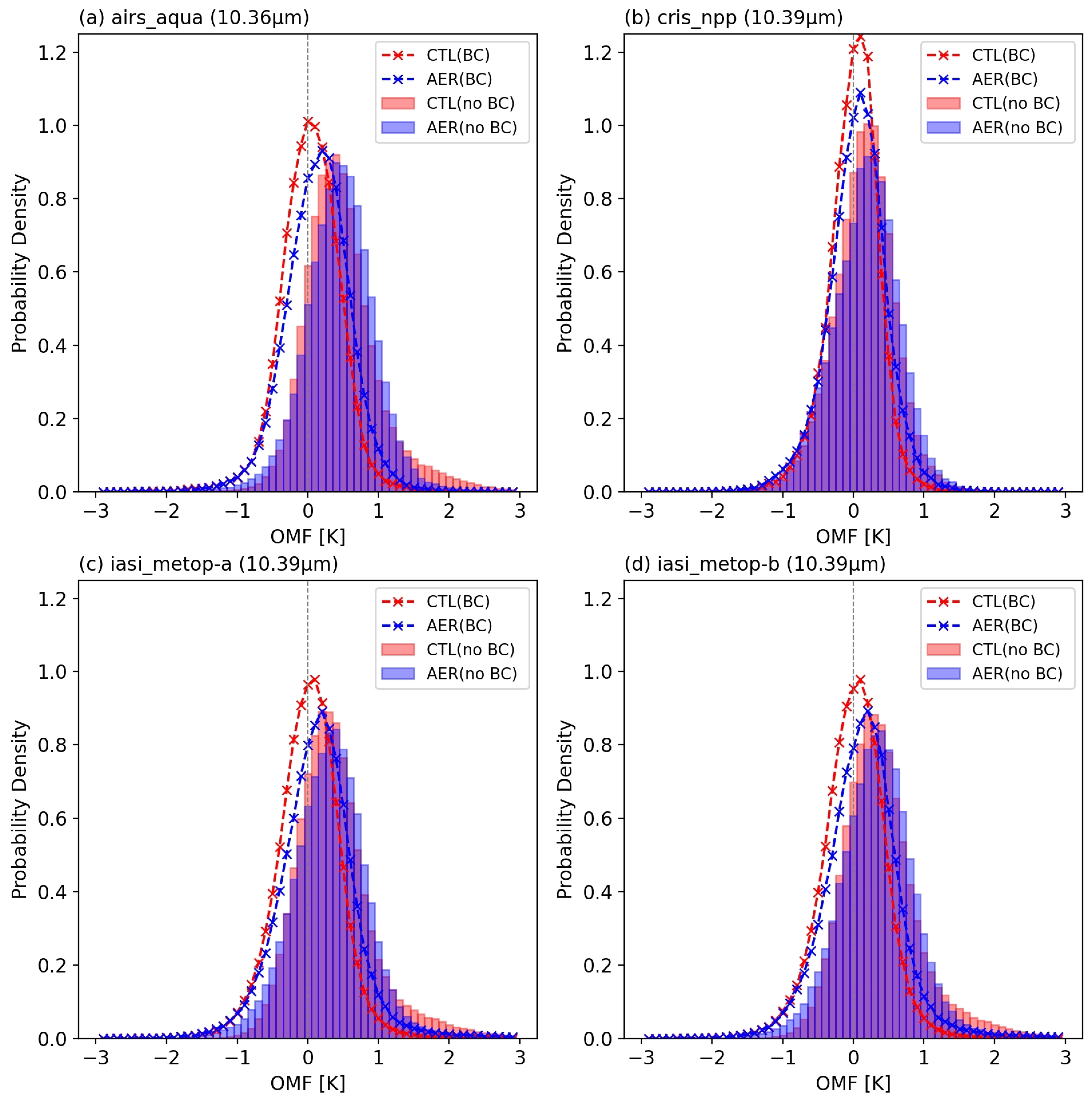
3.2. First-Guess Departure

The BT cooling effect shown in Figure 3 and Figure 4 subsequently affects the first-guess departures (OMFs) of BT which determine the analysis increments. Figure 5 illustrates the gridded monthly OMFs before QC and BC of IASI on MetOp-A at 10.39 μm for (a) CTL, (b) AER, and (c) the differences (i.e., AER minus CTL). Both CTL (Figure 5a) and AER (Figure 5b) have negative OMFs over most regions. This feature is mainly attributed to the cloud information not incorporated into the BT simulation under the clear-sky framework. Due to the cooler BTs simulated in AER, the OMF differences are globally positive in Figure 5c. It is statistically significant over the dust-impacted areas, such as the trans-Atlantic region, Sahara Desert, and Middle East. This indicates that the incorporation of aerosols in BT simulations shifts the OMFs toward more positive. As a result, AER will have larger positive analysis increments than CTL.
Figure 6 shows monthly mean OMFs (upper panel) and RMS OMFs (lower panel) before QC and BC from AIRS, Cross-track Infrared Sounder (CrIS), and IASI. Across most channels, all four high-spectral IR sensors have less negative mean OMFs in AER than CTL which is the same response as Figure 5 shown above. The smaller RMS OMFs indicate that considering aerosol radiance effect (i.e., AER) can improve the OMFs statistics through the entire thermal IR spectrum, especially the atmospheric window regions. Due to the identical first-guesses in CTL and AER, the standard deviation of mean and RMS OMFs along analysis cycles does not change significantly (not shown). It should be noted that cloud-affected observations were included in the statistics. Since clouds have stronger attenuation than aerosols, the impact of considering aerosol information in BT simulations on the statistics of OMFs is limited. The gap near 11.1 μm (900 cm−1) of AIRS on Aqua in Figure 6a is due to no available observations after screening out the unreasonable observed BT (around zero degree) at that particular channel.

3.3. Bias Correction and Quality Control

The BC algorithm in the GSI estimates and corrects the biases in the OMFs of radiance observations. Figure 7 illustrates the bias estimates gridded at 2.5° by 2.5° resolution for 10.39 μm of IASI on MetOp-A during August 2017. It includes the total biases in (a) CTL, (b) AER, and (c) the differences (AER minus CTL). Figure 7a displays that the CTL has globally positive values which means OMFs will decrease after the bias correction. In contrast, negative biases are estimated in AER (Figure 7b) over the Sahara Desert, South Asia, and the west Pacific, where aerosol loadings are higher (as shown in Figure 2). Together with OMFs statistics shown in Figure 5c, the OMFs of AER will become more positive than CTL over those regions. It should be noted that the land-sea difference is less significant in AER. Figure 7c indicates that the differences mainly distribute over land and the high latitude regions in both hemispheres.
Figure 8 shows the differences (i.e., AER minus CTL) of bias estimates contributed by temperature lapse rate and surface emissivity sensitivity predictors. Here only these two predictors are displayed because the change of bias estimates from other predictors are small. Figure 8a displays the result of lapse rate term which is estimated by the column integral of the product of layer differences of transmittance and temperature (   Δ τ × Δ T ). It shows that AER has smaller bias estimates over Africa and the trans-Atlantic regions. Since the first-guesses are identical in CTL and AER, the change of bias estimates of the lapse rate term is subjected to the change of the transmittance profile from CRTM due to the presence of aerosols. Figure 8b displays the results of surface emissivity sensitivity term which is estimated by the BT Jacobian for surface emissivity from CRTM. Please note that this term is only applied to the observations over the non-water surface, including the ice and snow surface at polar regions, to account for the uncertainties in surface types used in CRTM simulations. The significant reduction of this term in AER indicates that the BT Jacobian for surface emissivity is changed considerably after including aerosols into CRTM simulations. It also explains the less land-sea difference in AER (Figure 7b,c). In contrast to the lapse rate term, further study is needed to address how aerosols affect the calculation of BT Jacobian of surface emissivity in the CRTM.
In the GSI, the QC procedure (described in Section 2.1) checks the bias-corrected OMFs and determines the dataset involved in the minimization process. Table 2 lists the number of observations passed or rejected due to various QC checks for the CTL (top row) and AER (bottom row) at 10.39 μm for IASI on MetOp-A through 1–28 August 2017. Here we list the results of four QC checks used for this IASI channel. Only the observations that passed QC checks (the first column) were assimilated in the GSI. For this channel on IASI, the AER run assimilated fewer observations (cf. 235,997 vs. 262,758). It rejected more observations due to surface emissivity ( ϵ s f c ) and temperature ( T s f c ) sensitivity (cf. 259,595 vs. 166,291), but rejected less observations due to presence of cloud layers in model (cf. 572,345 vs. 638,676) than the CTL run. The larger OMF in AER also resulted in a small number of rejected observations due to the gross error check. Table 3 lists the changes in the QC results at 10.39 μm for IASI on MetOp-A in AER with respect to CTL. Considering aerosol information could change the QC results by about 21% of observations. For the assimilated observations in CTL, around 39% observations’ QC statistics were changed in AER. About 13% and 25% observations rejected in CTL due to clouds and ϵ s f c and T s f c sensitivity were changed, respectively. Moreover, most rejected observations in CTL due to physical temperature retrievals were changed in AER (89.8% in Table 3). These changes indicated that QC checks should be carefully addressed for assimilating aerosol-affected observations.
Figure 9 displays the horizontal distribution of OMFs rejected by the QC check of surface emissivity and temperature for the same cycle, channel, sensor, and region as Figure 4. Compared to CTL (Figure 9a), AER (Figure 9b) rejected more observations due to this QC check over mid-Atlantic, which contributes to the changes of QC statistics shown in the fifth column of Table 2. As documented in Liang and Weng [35], the QC check of surface emissivity and temperature for IR sensors is determined by a “skin temperature sensitivity related parameter”. The observation at a particular channel is rejected when the parameter is larger than 5% of channel observation error. Briefly, the parameter is proportional to the bias-corrected OMF which is larger in AER due to the cooling effect of BT simulations and the negative bias estimates over this region. Therefore, given the same observation error prescribed in AER and CTL, GSI tends to reject the observations with larger OMF (i.e., AER in this case).
The feature of more rejected observations over water at 10.39 μm in AER is shown in other sensors as well. Table 4 lists the count of the assimilated observations over different surface types (water, land, and mixed) for IASI, AIRS, and CrIS in CTL and AER near 10.4 μm during the period. IASI onboard MetOp-B and AIRS have a similar response as IASI onboard MetOp-A, less observations over water and more over land were assimilated in AER. However, the response is different for CrIS, where AER assimilated more observations over water than CTL at this channel. CrIS observations over land are not assimilated because the surface temperature sensitivity at this channel is higher than 0.2 (K/K) which is rejected in the QC procedure of CrIS. Overall, the total number of the assimilated data counts at this channel is reduced in AER.
The Gaussianity of probability density function (PDF) of OMFs is a common metric to qualitatively assess whether the biases in the assimilated dataset were removed properly through the BC algorithm. Figure 10 shows the PDFs between CTL and AER before BC (histograms) and after BC (dashed lines) near 10.39 μm for IASI, CrIS, and AIRS during 1–28 August 2017; all PDFs are computed based on the OMFs after QC. The histograms reflect that AER has more positive OMFs in all the four sensors. Comparing the BC influences on CTL and AER, the corrected PDFs of CTL peak at zero line which indicates that the BC algorithm properly removes the biases in OMFs. On the other hand, the pattern of the corrected PDFs skews toward positive slightly in AER. This indicates that BC coefficients from CTL may be unsuitable to estimate biases for aerosol-affected OMFs. Among the four sensors in AER, the OMFs of CrIS on Suomi-NPP (Figure 10b) are better corrected. This feature could be attributed to the rejection of the observations over land for CrIS by QC. It suggests that the BC algorithm may need some adjustment for using aerosol-affected observations over land.

3.4. Use of Observation

While the previous section focused on the response at a single channel, we would like to understand how the aerosol impacts on data usage vary with the assimilated channels and with the analysis cycles. For the response at different channels, Figure 11a shows the distribution of the data count differences (AER minus CTL) of assimilated observations from the 164 channels of IASI at each analysis cycle (i.e., every 6 h) during August 2017. When a box locates at the positive range in Figure 11a, it means that AER assimilated more observations from that channel in most analysis cycles. In the wavelengths from 9 to 13 μm, AER assimilates fewer observations than CTL in most analysis cycles. However, for the channels with longer wavelength, e.g., 13.5 to 14.5 μm, AER assimilates more data than CTL. As a result of compensation in data count difference between 9 to 13 μm and 13.5 to 14.5 μm, AER assimilates slightly more observations for IASI onboard MetOp-A. This is shown for each analysis cycle in Figure 11b, which displays the distribution of data count differences from all assimilated channels. When a box locates at the positive range in Figure 11b, it means AER assimilated more observations than CTL for the majority of assimilated channels at that analysis cycle. The mean of assimilated channels (red line) in Figure 11b indicates that the average number of assimilated observations in AER is slightly more than CTL at each analysis cycle.
Table 5 lists the average number of assimilated observations for the IR sensors. It also lists the average of differences (AER minus CTL), and their corresponding temporal (STDT) and spectral (STDS) standard deviations of differences. Larger value of STDT represents that the averaged difference of data count over assimilated channels varies considerably at each analysis cycle. Larger value of STDS represents that the averaged difference of data count over each analysis cycle varies considerably among each assimilated channel. For monitoring sensors, all available channels were included in the statistics. Table 5 shows that AER assimilates more observations than CTL from most IR sensors, except the Advanced Very High Resolution Radiometer (AVHRR) on MetOp-A and NOAA-18 and SEVIRI on Meteosat-10. The STDT differences among sensors also reflect the orbits of satellites. The sensors on polar orbiting satellites have larger STDT than geostationary satellites due to the heterogeneous distribution of aerosols. The larger STDS in IASI, CrIS, and AIRS could be attributed to the large set of assimilated channels which include aerosol sensitive and insensitive channels. Overall, the statistics indicate that more information contents from IR sensors were exploited in the AER experiment. This feature is primarily attributed to the channels of wavelength from 13.5 to 14.5 μm (Figure 11a) which are not measured in AVHRR and not the assimilated channel of SEVIRI in our experiments.

3.5. Temperature Analysis

Figure 12 presents the mean analysis difference between CTL and AER of (a) sea surface temperature and (b) temperature at 850 hPa. Also shown is the vertical cross-section of mean temperature differences (10° E–80° W) meridionally averaged over the northern tropics (0°–30° N)(Figure 12c). The differences indicate that analyzed SSTs in AER are about 0.3 to 0.5 K warmer than in CTL in the Atlantic Ocean (Figure 12a). This warming effect also extends to 850 hPa (Figure 12b) over Africa to the tropical Atlantic Ocean. However, there is a region with cooler 850 hPa temperatures near the Africa coast. Figure 12c indicates a warmer low level of atmosphere (∼0.15 K) crossing Africa to the Atlantic Ocean and a cooler mid-level over the Atlantic Ocean near Africa coast. This change of vertical temperature structure may induce more instability over this region. Consequently, the feature could affect the evolution of Africa easterly wave and the subsequent tropical cyclone activity.
The OMAs from in situ datasets (e.g., radiosonde, buoy, etc.) can be used to evaluate the analysis performance because the measurements are more accurate than remote sensing data. Figure 13 displays the scatterplots of SSTs between measurements and analysis over four regions with larger SST differences during August 2017. As shown in Figure 12a, the West Atlantic has the strongest warming effects (∼0.5 K); the East Atlantic region has the warming effects from 0.2–0.4 K; Arabian Sea region ranges around 0.1 to 0.2 K warming; West Pacific is about 0.2 K cooling in analyzed SSTs. The RMS and mean OMAs are labeled in the title of each panel.
The slope of four regression lines in each region implies that the analyzed SSTs in AER are a slightly better fit to the measurements except the West Atlantic. The coefficients of determination, R2, are similar over the four regions, which means that the analyzed SSTs are not significantly improved by considering aerosols in BT simulations. While there are no significant differences over these regions, the smaller RMS OMAs indicate that the SST analyses in AER are in better agreement with measurements. Also, the smaller absolute mean OMAs implies the AER experiment has reduced the warm biases in the West Pacific and the cold biases in other three regions. It should be noted that, compared to the large sampling size in the West Atlantic (>30,000 measurements), the other three regions have less than 100 measurements which could be less statistically meaningful, especially over the West Pacific (only 24 points during the entire period). O’Carroll et al. [53] reported that IASI SSTs have stronger cold biases than AVHRR SSTs against measurements from drifting buoys. Compare the SST retrieval methods from both, the aerosol corrections (e.g., the Saharan Dust Index from SEVIRI [19]) are applied in the retrieval method of AVHRR [54] but not in the method of IASI [55]. Similarly, cold biases of SST analyses in the CTL experiment can be reduced by considering aerosol information in BT simulations (i.e., AER).

4. Discussion and Conclusions

This study investigates the aerosol impacts on meteorological analysis by incorporating aerosol information into the radiance observation operator. Two GDAS experiments were conducted for 1–28 August 2017. These include an aerosol-blind cycling analysis experiment (CTL) and an aerosol-aware offline analysis experiment (AER). Overall, the aerosol-aware BT simulations lead to the following features in the AER run: (1) lower simulated BTs at the top of the atmosphere, (2) more positive OMFs, (3) more negative estimated biases, (4) considerable changes in the outcome of QC checks, (5) more IR observations assimilated, (6) warmer analyzed SST over the Atlantic Ocean and lower atmosphere over Africa to the central Atlantic Ocean, and (7) a slightly better agreement with SST measurements. In addition to the experiments presented in this study, a companion aerosol-aware cycling experiment was conducted. The results can be found at Grogan and Lu [56] and Wei et al. [57].
In terms of the aerosol information, there can be significant seasonal and annual variation of the loading, species, and vertical distribution in regions around the world. Also, the forecast errors of the aerosol model contribute uncertainties to the BT simulations. Our results suggest that cases with lower dust loading or dominated by a non-dust species would produce smaller cooling effects on the BT simulations. This would lead to smaller warming effects on the analyzed temperatures in the lower atmosphere. Future research should be conducted to comprehensively evaluate the effects of aerosols on the analysis system under a wider range of aerosol loading.
As the radiance observation operator in the GSI, the CRTM is the key component for direct assimilation of radiance observations. In this study, aerosol induced changes are driven by the aerosol-aware CRTM simulations, which uses the spherical assumption for aerosols. It has been recognized that non-spherical aerosols can affect the accuracy of radiance calculations in the IR window [58,59]. Hence, the spherical assumption could introduce uncertainties in our results. This issue has been addressed by the latest public release of the CRTM v2.4 (as of October 2020), which incorporates the non-spherical optical properties into the CRTM aerosol module. Nonetheless, the transmittance and Jacobians from the CRTM are incorporated into the BC, QC, and minimization processes for assimilating radiance observations in the GSI. It is still unclear how aerosols affect the CRTM simulation, the Jacobians in particular. Therefore, further investigation is needed to understand the response of the CRTM simulation to the presence of aerosols.
Our results showed that considering aerosol information in the CRTM reduced the discrepancies between the simulated and observed BTs. This in turn produced considerable changes in the outcome of QC checks and a more positive skewness in the PDFs of bias-corrected OMFs in the IR window region. Therefore, future studies are needed to explore the aerosol-aware QC and the aerosol-based BC predictor for assimilating aerosol-affected IR observations in the system. For aerosol-aware QC, an observation-based aerosol detection method can be used to identify the aerosol-affected IR observations. An aerosol-based BC predictor could be incorporated into the bias estimation to account for the uncertainties of the modeling aerosols in OMFs. These capabilities can constrain the aerosol effects on IR observations, and thus the aerosol-affected IR observations can be assimilated in the analysis system such as the all-sky DA approach for cloudy observations [60].

Author Contributions

Conceptualization, C.-H.L. and S.-W.W.; Investigation, S.-W.W., C.-H.L., Q.L., A.C., T.Z., X.L., J.W., R.G., and P.S.B.; Methodology, C.-H.L. and S.-W.W.; Software and visualization, S.-W.W.; Funding acquisition and project administration, C.-H.L.; Writing—original draft preparation, S.-W.W.; Writing—review and editing, S.-W.W., C.-H.L., and D.G. All authors have read and agreed to the published version of the manuscript.

Funding

The present work is funded by NOAA NWS NGGPS program (award number NA15NWS4680008).

Institutional Review Board Statement

Not applicable.

Informed Consent Statement

Not applicable.

Data Availability Statement

The data that supports the findings of this study is archived at NESDIS-funded Supercomputer for Satellite Simulations and Data Assimilation Studies (S4) cluster and can be made available to the readers upon request. The observations used in the GDAS experiment are available in the NCDC website (see text).

Acknowledgments

All code development and experiments are conducted at NESDIS-funded S4 cluster maintained by Space Science and Engineering Center (SSEC) at University of Wisconsin-Madison. All GDAS and NGAC data are provided by the operational archive at NCEP.

Conflicts of Interest

The authors declare no conflict of interest. The funders had no role in the design of the study; in the collection, analyses, or interpretation of data; in the writing of the manuscript, or in the decision to publish the results.

References

  1. Mitchell, J.M., Jr. The Effect of Atmospheric Aerosols on Climate with Special Reference to Temperature near the Earth’s Surface. J. Appl. Meteorol. 1971, 10, 703–714. [Google Scholar] [CrossRef] [Green Version]
  2. Twomey, S. Pollution and the Planetary Albedo. Atmos. Environ. 1974, 8, 1251–1256. [Google Scholar] [CrossRef]
  3. Twomey, S. The Influence of Pollution on the Shortwave Albedo of Clouds. J. Atmos. Sci. 1977, 34, 1149–1152. [Google Scholar] [CrossRef] [Green Version]
  4. Albrecht, B.A. Aerosols, Cloud Microphysics, and Fractional Cloudiness. Science 1989, 245, 1227–1230. [Google Scholar] [CrossRef] [PubMed]
  5. Jones, A.; Roberts, D.L.; Slingo, A. A climate model study of indirect radiative forcing by anthropogenic sulphate aerosols. Nature 1994, 370, 450–453. [Google Scholar] [CrossRef]
  6. Ackerman, A.S.; Toon, O.B.; Stevens, D.E.; Heymsfield, A.J.; Ramanathan, V.; Welton, E.J. Reduction of Tropical Cloudiness by Soot. Science 2000, 288, 1042–1047. [Google Scholar] [CrossRef] [Green Version]
  7. Lohmann, U.; Feichter, J.; Penner, J.; Leaitch, R. Indirect effect of sulfate and carbonaceous aerosols: A mechanistic treatment. J. Geophys. Res. Atmos. 2000, 105, 12193–12206. [Google Scholar] [CrossRef]
  8. Tompkins, A.M.; Cardinali, C.; Morcrette, J.-J.; Rodwell, M.J. Influence of aerosol climatology on forecasts of the African Easterly Jet. Geophys. Res. Lett. 2005, 32. [Google Scholar] [CrossRef] [Green Version]
  9. Pérez, C.; Nickovic, S.; Pejanovic, G.; Baldasano, J.M.; Özsoy, E. Interactive dust-radiation modeling: A step to improve weather forecasts. J. Geophys. Res. 2006, 111. [Google Scholar] [CrossRef] [Green Version]
  10. Rodwell, M.J.; Jung, T. Understanding the local and global impacts of model physics changes: An aerosol example. Q. J. R. Meteorol. Soc. 2008, 134, 1479–1497. [Google Scholar] [CrossRef]
  11. Mulcahy, J.P.; Walters, D.N.; Bellouin, N.; Milton, S.F. Impacts of increasing the aerosol complexity in the Met Office global numerical weather prediction model. Atmos. Chem. Phys. 2014, 14, 4749–4778. [Google Scholar] [CrossRef] [Green Version]
  12. Bozzo, A.; Remy, S.; Benedetti, A.; Flemming, J.; Bechtold, P.; Rodwell, M.J.; Morcrette, J.-J. Implementation of a CAMS-Based Aerosol Climatology in the IFS; ECMWF Tech. Memo; European Centre for Medium Range Weather Forecasts: Reading, UK, 2017; Volume 801.
  13. Nowottnick, E.P.; Colarco, P.R.; Braun, S.A.; Barahona, D.O.; da Silva, A.; Hlavka, D.L.; McGill, M.J.; Spackman, J.R. Dust Impacts on the 2012 Hurricane Nadine Track during the NASA HS3 Field Campaign. J. Atmos. Sci. 2018, 75, 2473–2489. [Google Scholar] [CrossRef] [PubMed]
  14. Highwood, E.J.; Haywood, J.M.; Silverstone, M.D.; Newman, S.M.; Taylor, J.P. Radiative Properties and Direct Effect of Saharan Dust Measured by the C-130 Aircraft during Saharan Dust Experiment (SHADE): 2. Terrestrial Spectrum. J. Geophys. Res. 2003, 108, 8578. [Google Scholar] [CrossRef] [Green Version]
  15. Köhler, C.H.; Trautmann, T.; Lindermeir, E.; Vreeling, W.; Lieke, K.; Kandler, K.; Weinzierl, B.; Groß, S.; Tesche, M.; Wendisch, M. Thermal IR Radiative Properties of Mixed Mineral Dust and Biomass Aerosol during SAMUM-2. Tellus B Chem. Phys. Meteorol. 2011, 63, 751–769. [Google Scholar] [CrossRef] [Green Version]
  16. Sokolik, I.N. The spectral radiative signature of wind-blown mineral dust: Implications for remote sensing in the thermal IR region. Geophys. Res. Lett. 2002, 29, 7-1–7-4. [Google Scholar] [CrossRef] [Green Version]
  17. Pierangelo, C.; Chedin, A.; Heilliette, S.; Jacquinet-Husson, N.; Armante, R. Dust altitude and infrared optical depth from AIRS. Atmos. Chem. Phys. 2004, 4, 1813–1822. [Google Scholar] [CrossRef] [Green Version]
  18. Matricardi, M. The Inclusion of Aerosols and Clouds in RTIASI, the ECMWF Fast Radiative Transfer Model for the Infrared Atmospheric Sounding Interferometer; ECMWF Tech. Memo; European Centre for Medium Range Weather Forecasts: Reading, UK, 2005; Volume 474.
  19. Merchant, C.J.; Embury, O.; Le Borgne, P.; Bellec, B. Saharan dust in nighttime thermal imagery: Detection and reduction of related biases in retrieved sea surface temperature. Remote Sens. Environ. 2006, 104, 15–30. [Google Scholar] [CrossRef]
  20. Liu, Q.; Han, Y.; van Delst, P.; Weng, F. Modeling aerosol radiance for NCEP data assimilation. In Fourier Transform Spectroscopy/Hyperspectral Imaging and Sounding of the Environment; HThA5; Optical Society of America: Washington, DC, USA, 2007. [Google Scholar] [CrossRef]
  21. Chen, Y.; Han, Y.; Weng, F. Comparison of two transmittance algorithms in the community radiative transfer model: Application to AVHRR. J. Geophys. Res. Atmos. 2012, 117. [Google Scholar] [CrossRef] [Green Version]
  22. Quan, X.; Huang, H.-L.; Zhang, L.; Weisz, E.; Cao, X. Sensitive detection of aerosol effect on simulated IASI spectral radiance. J. Quant. Spectrosc. Radiat. Transf. 2013, 122, 214–232. [Google Scholar] [CrossRef]
  23. Divakarla, M.; Barnet, C.; Goldberg, M.; Gu, D.; Liu, X.; Xiong, X.; Kizer, S.; Guo, G.; Wilson, M.; Maddy, E.; et al. Evaluation of CrIMSS operational products using in-situ measurements, model analysis fields, and retrieval products from heritage algorithms. In Proceedings of the 2012 IEEE International Geoscience and Remote Sensing Symposium, Munich, Germany, 22–27 July 2012; pp. 1046–1049. [Google Scholar]
  24. Letertre-Danczak, J. The Use of Geostationary Radiance Observations at ECMWF and Aerosol Detection for Hyper-Spectral Infrared Sounders: 1st and 2nd Years Report; EUMETSAT/ECMWF Fellowship Programme Research Reports; European Centre for Medium Range Weather Forecasts: Reading, UK, 2016; Volume 40.
  25. Geer, A.J.; Migliorini, S.; Matricardi, M. All-sky assimilation of infrared radiances sensitive to mid- and upper-tropospheric moisture and cloud. Atmos. Meas. Tech. Discuss. 2019, 12, 4903–4929. [Google Scholar] [CrossRef] [Green Version]
  26. Weaver, C.J.; Joiner, J.; Ginoux, P. Mineral aerosol contamination of TIROS Operational Vertical Sounder (TOVS) temperature and moisture retrievals. J. Geophys. Res. 2003, 108. [Google Scholar] [CrossRef] [Green Version]
  27. Kim, J.; Akella, S.; da Silva, A.M.; Todling, R.; McCarty, W. Preliminary Evaluation of Influence of Aerosols on the Simulation of Brightness Temperature in the NASA’s Goddard Earth Observing System Atmospheric Data Assimilation System; Tech. Rep. Ser. Glob. Model. Data Assim.; Goddard Space Flight Center, National Aeronautics and Space Administration: Greenbelt, MD, USA, 2018.
  28. Wang, X.; Lei, T. GSI-Based Four-Dimensional Ensemble—Variational (4DEnsVar) Data Assimilation: Formulation and Single-Resolution Experiments with Real Data for NCEP Global Forecast System. Mon. Weather Rev. 2014, 142, 3303–3325. [Google Scholar] [CrossRef]
  29. Kleist, D.T.; Ide, K. An OSSE-Based Evaluation of Hybrid Variational—Ensemble Data Assimilation for the NCEP GFS. Part II: 4DEnVar and Hybrid Variants. Mon. Weather Rev. 2015, 143, 452–470. [Google Scholar] [CrossRef] [Green Version]
  30. Lorenc, A.C.; Rawlins, F. Why Does 4D-Var Beat 3D-Var? Q. J. R. Meteorol. Soc. 2005, 131, 3247–3257. [Google Scholar] [CrossRef]
  31. Weng, F.; Han, Y.; van Delst, P.; Liu, Q.; Kleespies, T.; Yan, B.; Marshall, J.L. JCSDA Community Radiative Transfer Model (CRTM). In Proceedings of the 14th International TOVS Study Conference, BeiJing, China, 25–31 May 2005; p. 6. [Google Scholar]
  32. Han, Y.; van Delst, P.; Liu, Q.; Weng, F.; Yan, B.; Treadon, R.; Derber, J. JCSDA Community Radiative Transfer Model (CRTM)—Version 1; NOAA Technical Report NESDIS; National Oceanic and Atmospheric Administration National Environmental Satellite, Data, and Information Service: Washington, DC, USA, 2006; Volume 122.
  33. Derber, J.C.; Wu, W.-S. The Use of TOVS Cloud-Cleared Radiances in the NCEP SSI Analysis System. Mon. Weather Rev. 1998, 126, 2287–2299. [Google Scholar] [CrossRef]
  34. Zhu, Y.; Derber, J.; Collard, A.; Dee, D.; Treadon, R.; Gayno, G.; Jung, J.A. Enhanced radiance bias correction in the National Centers for Environmental Prediction’s Gridpoint Statistical Interpolation data assimilation system: Radiance Bias Correction in GSI. Q. J. R. Meteorol. Soc. 2014, 140, 1479–1492. [Google Scholar] [CrossRef]
  35. Liang, D.; Weng, F. Evaluation of the impact of a new quality control method on assimilation of CrIS data in HWRF-GSI. In Proceedings of the 2014 IEEE Geoscience and Remote Sensing Symposium, Quebec City, QC, Canada, 13–18 July 2014; pp. 3778–3781. [Google Scholar]
  36. Gemmill, W.; Katz, B.; Li, X.; Burroughs, L.D. The Daily Real-Time, Global Sea Surface Temperature—High Resolution Analysis: RTG_SST_HR. Tech. Proc. Bull. 2006, 10, 1–39. [Google Scholar]
  37. Liu, Q.; Weng, F. Advanced Doubling—Adding Method for Radiative Transfer in Planetary Atmospheres. J. Atmos. Sci. 2006, 63, 3459–3465. [Google Scholar] [CrossRef]
  38. Ding, S.; Yang, P.; Weng, F.; Liu, Q.; Han, Y.; van Delst, P.; Li, J.; Baum, B. Validation of the Community Radiative Transfer Model. J. Quant. Spectrosc. Radiat. Transf. 2011, 112, 1050–1064. [Google Scholar] [CrossRef]
  39. Li, J.; Li, Z.; Wang, P.; Schmit, T.J.; Bai, W.; Atlas, R. An Efficient Radiative Transfer Model for Hyperspectral IR Radiance Simulation and Applications under Cloudy-sky Conditions. J. Geophys. Res. Atmos. 2017, 122, 7600–7613. [Google Scholar] [CrossRef]
  40. Hess, M.; Koepke, P.; Schult, I. Optical Properties of Aerosols and Clouds: The Software Package OPAC. Bull. Am. Meteorol. Soc. 1998, 79, 831–844. [Google Scholar] [CrossRef]
  41. Liu, Q.; Lu, C.-H. Community Radiative Transfer Model for Air Quality Studies. In Light Scattering Reviews; Kokhanovsky, A., Ed.; Springer Praxis Books; Springer: Berlin/Heidelberg, Germany, 2016; Volume 11, pp. 67–115. [Google Scholar]
  42. Lu, C.-H.; da Silva, A.; Wang, J.; Moorthi, S.; Chin, M.; Colarco, P.; Tang, Y.; Bhattacharjee, P.S.; Chen, S.-P.; Chuang, H.-Y.; et al. The implementation of NEMS GFS Aerosol Component (NGAC) Version 1.0 for global dust forecasting at NOAA/NCEP. Geosci. Model Dev. 2016, 9, 1905–1919. [Google Scholar] [CrossRef] [PubMed] [Green Version]
  43. Wang, J.; Bhattacharjee, P.S.; Tallapragada, V.; Lu, C.-H.; Kondragunta, S.; da Silva, A.; Zhang, X.; Chen, S.-P.; Wei, S.-W.; Darmenov, A.S.; et al. The implementation of NEMS GFS Aerosol Component (NGAC) Version 2.0 for global multispecies forecasting at NOAA/NCEP—Part 1: Model descriptions. Geosci. Model Dev. 2018, 11, 2315–2332. [Google Scholar] [CrossRef] [Green Version]
  44. Zhang, L.; Grell, G.A.; Montuoro, R.; McKeen, S.A.; Bhattacharjee, P.S.; Baker, B.; Henderson, J.; Pan, L.; Frost, G.J.; McQueen, J.; et al. Development of GEFS-Aerosols into NOAAs Unified Forecast System UFS. Geosci. Model Dev. 2020. to be submitted. [Google Scholar]
  45. Chin, M.; Rood, R.B.; Lin, S.-J.; Müller, J.-F.; Thompson, A.M. Atmospheric sulfur cycle simulated in the global model GOCART: Model description and global properties. J. Geophys. Res. Atmos. 2000, 105, 24671–24687. [Google Scholar] [CrossRef]
  46. Colarco, P.; da Silva, A.; Chin, M.; Diehl, T. Online simulations of global aerosol distributions in the NASA GEOS-4 model and comparisons to satellite and ground-based aerosol optical depth. J. Geophys. Res. 2010, 115. [Google Scholar] [CrossRef] [Green Version]
  47. Bhattacharjee, P.S.; Wang, J.; Lu, C.-H.; Tallapragada, V. The implementation of NEMS GFS Aerosol Component (NGAC) Version 2.0 for global multispecies forecasting at NOAA/NCEP—Part 2: Evaluation of aerosol optical thickness. Geosci. Model Dev. 2018, 11, 2333–2351. [Google Scholar] [CrossRef] [Green Version]
  48. Ota, Y.; Derber, J.C.; Kalnay, E.; Miyoshi, T. Ensemble-Based Observation Impact Estimates Using the NCEP GFS. Tellus A Dyn. Meteorol. Oceanogr. 2013, 65, 20038. [Google Scholar] [CrossRef]
  49. Groff, D. Assessment of ensemble Forecast sensitivity to Observation (eFsO) Quantities for satellite Radiances Assimilated in the 4DenVar GFs. JCSDA Q. 2017, 54, 1–5. [Google Scholar] [CrossRef]
  50. Cardinali, C. Forecast Sensitivity Observation Impact with an Observation-Only Based Objective Function. Q. J. R. Meteorol. Soc. 2018, 144, 2089–2098. [Google Scholar] [CrossRef]
  51. Diniz, F.L.R.; Todling, R. Assessing the Impact of Observations in a Multi-year Reanalysis. Q. J. R. Meteorol. Soc. 2020, 146, 724–747. [Google Scholar] [CrossRef]
  52. Hilton, F.; Armante, R.; August, T.; Barnet, C.; Bouchard, A.; Camy-Peyret, C.; Capelle, V.; Clarisse, L.; Clerbaux, C.; Coheur, P.-F.; et al. Hyperspectral Earth Observation from IASI: Five Years of Accomplishments. Bull. Am. Meteor. Soc. 2012, 93, 347–370. [Google Scholar] [CrossRef]
  53. O’Carroll, A.G.; August, T.; Le Borgne, P.; Marsouin, A. The Accuracy of SST Retrievals from Metop-A IASI and AVHRR Using the EUMETSAT OSI-SAF Matchup Dataset. Remote Sens. Environ. 2012, 126, 184–194. [Google Scholar] [CrossRef]
  54. Le Borgne, P.; Legendre, G.; Marsouin, A.; Péré, S. Operational SST Retrieval from METOP/AVHRR Validation Report, version 2.0; Ocean and Sea-Ice SAF CDOP Report; Météo-France/DP/CMS: Lannion, France, 2008. [Google Scholar]
  55. August, T.; Klaes, D.; Schlüssel, P.; Hultberg, T.; Crapeau, M.; Arriaga, A.; O’Carroll, A.; Coppens, D.; Munro, R.; Calbet, X. IASI on Metop-A: Operational Level 2 Retrievals after Five Years in Orbit. J. Quant. Spectrosc. Radiat. Transf. 2012, 113, 1340–1371. [Google Scholar] [CrossRef]
  56. Grogan, D.; Lu, C.-H. Impacts of Aerosols on Meteorological Assimilation: A Case Study for the African Easterly Wave that Developed Hurricane Harvey. JCSDA Q. 2020, 67, 12–18. [Google Scholar] [CrossRef]
  57. Wei, S.-W.; Collard, A.; Grumbine, R.; Liu, Q.; Lu, C.-H. Impacts of Aerosols on Simulated Brightness Temperature and Analysis Fields. JCSDA Q. 2020, 67, 7–12. [Google Scholar] [CrossRef]
  58. Otto, S.; Trautmann, T.; Wendisch, M. On Realistic Size Equivalence and Shape of Spheroidal Saharan Mineral Dust Particles Applied in Solar and Thermal Radiative Transfer Calculations. Atmos. Chem. Phys. 2011, 11, 4469–4490. [Google Scholar] [CrossRef] [Green Version]
  59. Klüser, L.; Di Biagio, C.; Kleiber, P.D.; Formenti, P.; Grassian, V.H. Optical Properties of Non-Spherical Desert Dust Particles in the Terrestrial Infrared—An Asymptotic Approximation Approach. J. Quant. Spectrosc. Radiat. Transf. 2016, 178, 209–223. [Google Scholar] [CrossRef] [Green Version]
  60. Zhu, Y.; Liu, E.; Mahajan, R.; Thomas, C.; Groff, D.; Van Delst, P.; Collard, A.; Kleist, D.; Treadon, R.; Derber, J.C. All-Sky Microwave Radiance Assimilation in NCEP’s GSI Analysis System. Mon. Weather Rev. 2016, 144, 4709–4735. [Google Scholar] [CrossRef]
Figure 1. The diagram of the procedures for radiance observations in an analysis cycle of GSI. (a) is the aerosol-blind cycling experiment (CTL). (b) is the aerosol-aware offline experiment (AER). The orange boxes indicate the data processed in the GSI.
Atmosphere 12 00432 g001
Figure 2. Mean AOD at 550 nm of (a) dust (b) sea salt (c) carbonaceous and (d) sulfate aerosols from NGAC v2 over 1–28 August 2017.
Atmosphere 12 00432 g002
Figure 3. Average simulated brightness temperature (BT) differences for high-spectral IR sensors between AER and CTL (AER minus CTL) as a function of wavenumber (cm −1). The observations before BC and QC where NGAC v2 AOD at 550 nm > 0.3 and species fraction > 0.65 over 1–28 August 2017 are included in statistics. (a) dust, (b) sea salt, (c) carbonaceous, and (d) sulfate aerosols.
Atmosphere 12 00432 g003
Figure 4. Comparison of BT at 10.39 μm of IASI on MetOp-A between CTL and AER at the cycle of August 5 12Z, 2017. (a) BT of observations (b) simulated BTs of CTL (c) simulated BTs of AER (d) BTs differences between CTL and AER. The AOD at 550 nm contour lines of 0.1, 0.2, and 0.3 are plotted in brown.
Atmosphere 12 00432 g004
Figure 5. Comparison of first-guess departures before BC and QC at 10.39 μm from IASI on MetOp-A gridded at 2.5° by 2.5° over 1–28 August 2017. (a) CTL (b) AER (c) differences (AER minus CTL). Stippling in (c) indicates the difference is 99% significant (p ≤ 0.01).
Atmosphere 12 00432 g005
Figure 6. Mean OMFs (upper panel in each) and RMS OMFs (lower panel in each) before BC and QC on (a) AIRS on Aqua (b) CrIS on Suomi-NPP (c) IASI on MetOp-A and (d) IASI on MetOp-B averaged along analysis cycles during 1–28 August 2017. Results of CTL and AER are presented in red and blue, respectively.
Atmosphere 12 00432 g006
Figure 7. Comparison of estimated biases at 10.39 μm of IASI on MetOp-A gridded at 2.5° by 2.5° over 1–28 August 2017. (a) total biases of CTL (b) total biases of AER (c) total difference between AER and CTL (AER minus CTL). Stippling in (c) indicates the difference is 99% significant (p ≤ 0.01).
Atmosphere 12 00432 g007
Figure 8. Same as Figure 7, but for bias estimates differences (AER minus CTL) from the predictors of (a) lapse rate term and (b) emissivity term. Stippling indicates the difference is 99% significant (p ≤ 0.01).
Atmosphere 12 00432 g008
Figure 9. The distribution of rejected OMFs due to surface emissivity and temperature check for (a) CTL and (b) AER at the cycle of 12Z 5 August 2017. The data count is shown in the title of each panel. The AOD at 550 nm contour lines of 0.1, 0.2, and 0.3 are plotted in brown.
Atmosphere 12 00432 g009
Figure 10. Probability density function of first-guess departures over all assimilated observations (after QC) of CTL (red) and AER (blue) near 10.3 μm on (a) AIRS on Aqua (b) CRIS on Suomi-NPP (c) IASI on MetOp-A and (d) IASI on MetOp-B during 1–28 August 2017. Dashed lines stand for the results after BC, whereas histograms stand for the results before BC.
Atmosphere 12 00432 g010
Figure 11. Boxplots for assimilated observation number difference (AER minus CTL) from IASI on MetOp-A in (a) the distribution of analysis cycles along assimilated channels and (b) the distribution of assimilated channels along analysis cycles. The 5th, 25th, 50th, 75th, and 95th percentile are displayed. Red line in (b) is the average value over all the assimilated channels.
Atmosphere 12 00432 g011
Figure 12. Mean analysis difference (AER minus CTL) on (a) sea surface temperature, (b) 850 hPa temperature, and (c) cross section of temperature meridional mean from 0° to 30° N at 1° by 1° averaged over 1–28 August 2017.
Atmosphere 12 00432 g012
Figure 13. Scatter plots of the analyzed sea surface temperature against the ingested measurements over (a) West Atlantic, (b) East Atlantic (c) Arabian Sea, and (d) West Pacific. Corresponding areas are indicated in the lower left panel. Mean and RMS OMAs are indicated in the caption of each panel.
Atmosphere 12 00432 g013
Table 1. The information of thermal infrared sensors ingested into GDAS.
IR InstrumentSatelliteAssimilated/Subset Channels NumberECT */Location
Sun-synchronous
  AIRSAqua117/28113:30 asc
  AVHRRMetOp-A3/308:46 desc
  AVHRRNOAA-183/319:15 asc
  CrISSuomi-NPP82/39913:25 asc
  HIRS4MetOp-A0/1908:46 desc
  HIRS4MetOp-B0/1909:30 desc
  HIRS4NOAA-190/1915:15 asc
  IASIMetOp-A164/61608:46 desc
  IASIMetOp-B164/61609:30 desc
Geostationary
  SEVIRIMeteosat-80/841.5° E
  SEVIRIMeteosat-102/89.5° E
  SNDRD1GOES-1515/18128° W
  SNDRD2GOES-1515/18128° W
  SNDRD3GOES-1515/18128° W
  SNDRD4GOES-1515/18128° W
* ECT: Equatorial Crossing Time, asc: ascend orbit, desc: descend orbit.
Table 2. The count of observations categorized by QC checks at 10.39 μm of IASI onboard MetOp-A from CTL (top row) to AER (bottom row) during 1–28 August 2017. The total number of observations is 1,068,286.
PassedRejected (Gross Error)Rejected (Cloud)Rejected (Phys. Temp.) *Rejected ( ϵ sfc & T sfc ) *
CTL262,758 (24.6%)0 (0%)638,676 (59.8%)561 (0.05%)166,291 (15.6%)
AER235,997 (22.1%)9 (<0.01%)572,345 (53.6%)340 (0.03%)259,595 (24.3%)
* Phys. Temp.: physical temperature retrieval, ϵ sfc : surface emissivity, T sfc : surface temperature.
Table 3. The changes in the QC results in AER at 10.39 μm of IASI onboard MetOp-A with respect to CTL. The percentage relative to the counts in CTL is indicated in the parenthese.
PassedRejected
(Gross Error)
Rejected
(Cloud)
Rejected
(Phys. Temp.) *
Rejected
( ϵ sfc & T sfc ) *
Total
Unchanged161,045
(61.3%)
0 (0%)554,806
(86.9%)
57
(10.2%)
123,627
(74.3%)
839,535
(78.6%)
Changed101,713
(38.7%)
0 (0%)83,870
(13.1%)
504
(89.8%)
42,644
(25.7%)
228,
(21.4%)
* Phys. Temp.: physical temperature retrieval, ϵ s f c : surface emissivity, T s f c : surface temperature.
Table 4. Comparison of the count of assimilated observations over different surface type at 10.39 μm of IASI on MetOp-A and -B, CrIS onboard Suomi-NPP, and 10.36 μm of AIRS onboard Aqua for period 1–28 August 2017 in CTL and AER. The percentage of the total amount of each sensor is indicated in the parenthese.
SensorsCTLAER
WaterLandMixedWaterLandMixed
IASI (MetOp-A)219,368
(20.5%)
31,977
(3.0%)
11,413
(1.1%)
183,886
(17.2%)
39,157
(3.7%)
12,954
(1.2%)
IASI (MetOp-B)226,738
(20.4%)
33,044
(3.0%)
11,949
(1.1%)
190,190
(17.1%)
39,880
(3.6%)
12,983
(1.1%)
AIRS (Aqua)131,125
(17.5%)
15,002
(2.0%)
9470
(1.3%)
124,116
(16.6%)
18,955
(2.6%)
8346
(1.1%)
CrIS (Suomi-NPP)55,821
(4.2%)
050
(<0.01%)
65,278
(4.9%)
036
(<0.01%)
Table 5. Average assimilated observations number among infrared sensors over 1–28 August 2017. Rows below the dash line are monitored-only sensors. STDT and STDS stand for the temporal and spectral standard deviation of difference between AER and CTL, respectively. The relative changes of each sensor in AER are indicated in the parenthese.
SensorsCTLAERAER – CTL
AverageAverageAverageSTDTSTDS
high-spectral IR sensors
  IASI (MetOp-A)5810.725871.5460.81 (+1.05%)79.03256.56
  IASI (MetOp-B)5875.535937.9162.38 (+1.06%)81.33264.09
  CrIS (Suomi-NPP)3502.793510.667.87 (+0.22%)95.31255.08
  AIRS (Aqua)4188.224314.35126.13 (+3.01%)72.64157.61
low-spectral IR sensors
  AVHRR (MetOp-A)2516.392462.29−54.11 (−2.15%)112.6577.96
  AVHRR (NOAA-18)2221.322183.97−37.35 (−1.68%)93.6870.99
  SEVIRI (Meteosat-10)3607.363591.91−15.45 (−0.43%)14.907.07
  SNDRD1 (GOES-15)353.30394.5641.26 (+11.68%)30.2736.80
  SNDRD2 (GOES-15)368.99412.4643.46 (+11.78%)34.2841.05
  SNDRD3 (GOES-15)363.76403.7940.03 (+11.00%)33.1239.83
  SNDRD4 (GOES-15)376.28416.7940.51 (+10.77%)33.3641.59
  HIRS4 (NOAA-19)3167.083390.80223.72 (+7.06%)72.00235.43
  HIRS4 (MetOp-A)3176.413203.6027.20 (+0.86%)78.64211.69
  HIRS4 (MetOp-B)3104.203382.96278.76 (+8.98%)67.12231.49
  SEVIRI (Meteosat-8)1820.231773.75−46.48 (−2.55%)24.4344.64
Publisher’s Note: MDPI stays neutral with regard to jurisdictional claims in published maps and institutional affiliations.

