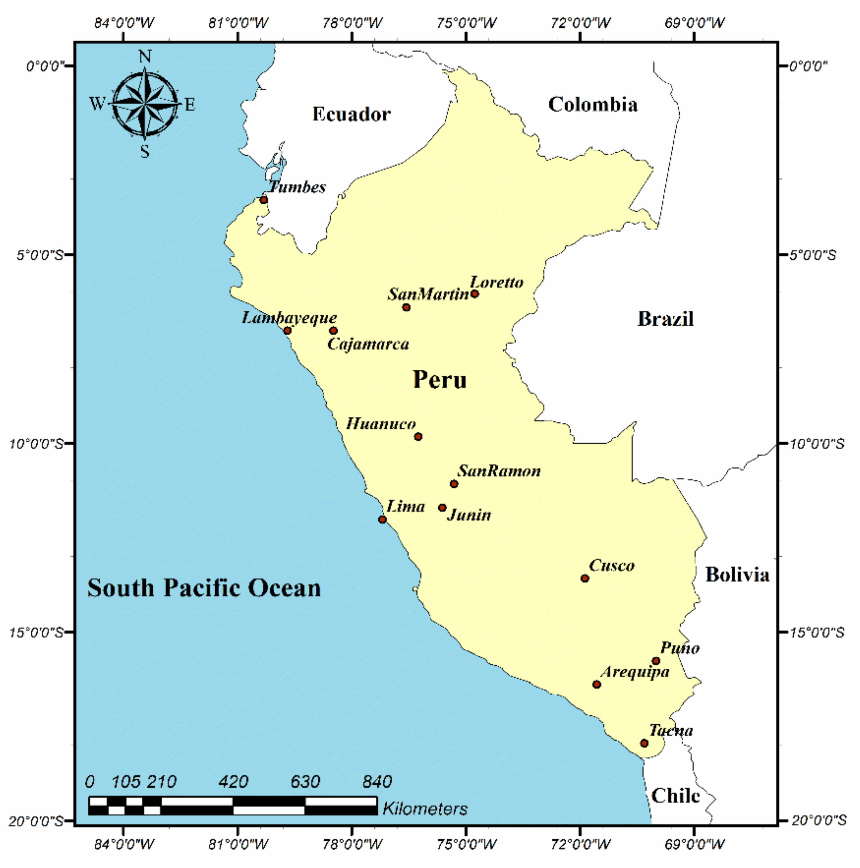
Review

Performance Analysis of Daily Global Solar Radiation Models in Peru by Regression Analysis

by
Babak Mohammadi
1,* and
Roozbeh Moazenzadeh
2,*
1
Department of Physical Geography and Ecosystem Science, Lund University, Sölvegatan 12, SE-223 62 Lund, Sweden
2
Department of Water Engineering, Faculty of Agriculture, Shahrood University of Technology, Shahrood 36199-95161, Iran
*
Authors to whom correspondence should be addressed.
Atmosphere 2021, 12(3), 389; https://doi.org/10.3390/atmos12030389
Submission received: 21 February 2021 / Revised: 11 March 2021 / Accepted: 13 March 2021 / Published: 17 March 2021
(This article belongs to the Special Issue Advances in Atmospheric Sciences)

Abstract

:
Solar radiation (Rs) is one of the main parameters controlling the energy balance at the Earth’s surface and plays a major role in evapotranspiration and plant growth, snow melting, and environmental studies. This work aimed at evaluating the performance of seven empirical models in estimating daily solar radiation over 1990–2004 (calibration) and 2004–2010 (validation) at 13 Peruvian meteorological stations. With the same variables used in empirical models (temperature) as well as two other parameters, namely precipitation and relative humidity, new models were developed by multiple linear regression analysis (proposed models). In calibration of empirical models with the same variables, the lowest estimation errors were 227.1 and 236.3 J·cm−2·day−1 at Tacna and Puno stations, and the highest errors were 3958.4 and 3005.7 at San Ramon and Junin stations, respectively. The poorest-performing empirical models greatly overestimated Rs at most stations. The best performance of a proposed model (in terms of percentage of error reduction) was 73% compared to the average of all empirical models and 93% relative to the poorest result of empirical models, both at San Ramon station. According to root mean square errors (RMSEs) of proposed models, the worst and the best results are achieved at San Martin station (RMSE = 508.8 J·cm−2·day−1) and Tacna station (RMSE = 223.2 J·cm−2·day−1), respectively.

1. Introduction

Solar radiation reaching Earth’s surface is one of the main sources of clean and renewable energy, optimal use of which can reduce human dependence on fossil fuels that contribute substantially to global warming [1,2]. The energy from Rs is the source of many processes on our planet, to the point that human life depends on it. Rs is an important topic in various areas of study such as hydrology [3,4,5], environmental science [6,7,8,9], water resources management [10,11], water balance modeling [12,13], and plant growth modeling [14,15,16,17]. This parameter is widely used in meteorological forecast models, climate change models, and ecosystem models [18,19,20,21,22]. It also plays a prominent role in such important processes as evaporation, evapotranspiration, and snowmelt. Knowing daily values of Rs and how it changes in the long-term can help researchers (in development of theoretical studies) and technologists (in assessment of the equipment associated with solar energy, for example, in designing photovoltaic systems and solar panels or thermal systems).
Rs is directly measured in meteorological stations using pyranometers. In contrast to other major meteorological parameters which are readily available (temperature, humidity, and precipitation, for instance), the high cost and difficulty in maintenance and calibration of pyranometers have led to a lack of reliable data for this parameter in many developing countries, and this adversely impacts research activities which depend on it. Due to such constraints, Rs is indirectly estimated using various methods.
Day of the year-based methods, conventional methods (e.g., empirical models), and new soft computing methods (e.g., Artificial Intelligence—AI) have been among the most important and most widely used methods for estimating Rs. In day of the year-based methods, generally sine wave functions [23], cosine wave functions [24], combined sine-cosine wave functions [25], polynomial functions [26], or Gaussian functions [27] are fitted to Rs values measured over a long timeframe, and no meteorological parameters are used [28,29]. Quej et al. [1] assessed the performance of four existing models as well as their own proposed Gaussian model in terms of estimating Rs at six meteorological stations in Mexico and reported root mean square errors (RMSEs) ranging between 97.5 and 219.7 J·cm−2·day−1.
Empirical models are typically employed in the form of temperature-based [30,31,32,33], sunshine-based [34,35], or hybrid models [33,36] in which the relation between inputs and output (Rs) is based on linear and nonlinear regression analysis or polynomial functions. Hassan et al. [20] evaluated empirical models over a 20-year time period in Egypt and subsequently developed new models, the best of which had a mean absolute percentage error (MAPE) of approximately 2.87%. Yildirim et al. [37] used different empirical models for estimating Rs in three stations in Turkey and also developed new models for which RMSE ranged between 1.183 and 1.569, respectively. In an extensive study, 732 empirical models and 65 functional forms for estimating Rs in different parts of Africa were reviewed by Chukwujindu [38].
Although new soft computing methods including artificial intelligence, for example, artificial neural networks (ANN), adaptive neuro-fuzzy inference system (ANFIS), support vector machine (SVM) and extreme learning machine (ELM), and their coupling with relative novel optimization algorithms such as particle swarm optimization (PSO), firefly algorithm (FA), and whale optimization algorithm (WOA) have improved the performance of Rs estimation in recent years, they require considerable user knowledge and are also more complex compared to empirical models [39,40,41,42,43,44,45,46,47]. Tymvios et al. [48] reported better performance of ANN (seven different architectures with best RMSE = 10.15) compared to Angstrom model (three different types with best RMSE = 13.36). Rahimikhoob [49] compared Hargreaves-Samani and a new ANN model in a semiarid region and reported better results for ANN model with RMSE and R2 values of 253.4 J·cm−2·day−1 and 0.89, respectively. Behrang et al. [50] evaluated multilayer perceptron (MLP) and radial basis function (RBF) neural networks under six scenarios in Dezful, Iran and reported MAPEs varying between 5.21 and 12.86% and 5.56 and 12.39% for MLP and RBF, respectively.
Multilinear regression (MLR), multi-nonlinear regression (MNLR) and feed-forward artificial neural network methods were used by Bilgili and Ozgoren [51] for modeling daily total Rs in Adana, Turkey, with MAPE and R2 values of 9.23% and 97.5%, respectively. Khatib et al. [52] examined performance of linear, nonlinear, fuzzy logic and ANN models in estimating Rs at five sites in Malaysia and reported MAPEs of 8.13, 6.93, 6.71 and 5.38%, respectively. A comprehensive review of different types of ANN and different input variables is provided by Yadav and Chandel [46].
Recently, researchers reported ability of machine learning approaches for solar radian estimating. Kisi [53] reported a new model by fuzzy genetic model for the estimation of solar radiation in Turkey. The provided model reported the better results during the testing stage and outperformed the other machine learning models used. In another study, Mohammadi and Aghashariatmadari [4] coupled support vector regression via krill-herd optimization algorithm. They reported a satisfied result by RMSE between 3.96 and 1.98 (MJ·m−2·day−1) for new proposed model for daily solar ration in Iran. Aybar-Ruiz et al. [54] used a coupled model via Grouping Genetic Algorithm enhanced by an extreme learning machine (ELM) for solar radiation estimation. The results showed that new hybrid model was more accurate than the ordinary ELM model. Ibrahim and Khatib [55] integrated the Random Forest (RF) model by Firefly optimization algorithm (FFA) for solar radiation estimation in Malaysia. The proposed new model (RF-FFA) was compared to ordinary artificial neural network (ANN), hybrid ANN-FFA, and standalone RF model; finally, they reported satisfied results for all machine learning model used. Capability of ANN, genetic programming (GP), and support vector machine coupled with firefly algorithm (SVM-FFA) for predicting Rs was examined in three locations in Nigeria with best results (RMSE = 1.866; R2 = 0.73) for SVM-FFA [56]. Accuracy of empirical, ANN, and SVM models in estimating Rs using most influencing meteorological parameters in India was assessed by Meenal and Selvakumar [47]. The lowest and highest RMSEs were 0.6387 (sunshine-based models) and 2.4328 (temperature-based models) for empirical models, 0.5814 (hybrid models) and 2.2197 (temperature-based models) for ANN and 0.4205 (hybrid models), and 1.1434 (temperature-based models) for SVM. Zang et al. [57] assessed the performance of 14 day of the year-based models in 35 Chinese meteorological stations. These included seven empirical models (six from the literature and one proposed model) and seven machine learning models (support vector regression (SVR), Gaussian process regression (GPR), three ANFIS models, and two ANFIS models coupled with chaotic firefly algorithm (CFA) and whale optimization algorithm with simulated annealing and roulette wheel selection (WOASAR)). ANFIS-CFA and ANFIS-WOASAR showed the highest accuracy in 19 and 15 stations, with RMSEs and MAPEs in the ranges 1.203–2.491 MJ·m2 and 4.516–18.976%, respectively. A relatively comprehensive review on application of machine learning methods is provided by Voyant et al. [58].
The particular geographic location of Peru (on the southern hemisphere), reliance of its economy on the agricultural industry, and the absence of a comprehensive study on Rs estimation in this country highlight the importance of accurate estimation of this parameter in Peru. Due to the lack of recorded sunshine hour data, the main objective of the present study was to evaluate the performance of seven empirical models (six temperature-based models and one temperature-precipitation based model) in estimating daily Rs values over 1990–2010 in 13 Peruvian meteorological stations. The authors also intended to develop and validate new empirical models based on recorded meteorological data in each station (proposed models) for improving Rs estimation if none of the available models would prove to be suitable.

2. Materials and Methods

2.1. Study Area

Peru has a total area of 1,280,000 square kilometers, spanning from 0° to 18° S and from 69° to 82° W, its average altitude is 2650 m above sea level, and it is bounded by the South Pacific Ocean to the east (Figure 1). The Andes mountain range extends from north to south and divides the country into three parts: a mountainous region with sunlit valleys and 6000 m peaks, a narrow desert and lowland zone between the mountains and the Pacific Ocean, and a lowland, wet, and very warm region on the eastern side of the mountainous area. Eastern Peru is covered by tropical rainforests (Amazonia) with a very high precipitation. With Lake Titicaca (the highest navigable lake in the world) on the south-eastern part and along the border with Bolivia, Atacama Desert (the driest place on Earth) along the border with Chile, and Sechura Desert on the northwest along the Pacific Ocean coast, the country has a unique weather profile.
Peruvian economy relies on the agriculture industry. Knowing the quantity, distribution, and dynamics of Rs across the country will therefore significantly contribute to irrigation scheduling and water resources management. Accurate estimation of this parameter will also be useful in sustainable solar energy generation by helping in the design of solar panels, solar thermal systems, and photovoltaic systems.

2.2. Empirical Models

Using daily recorded meteorological parameters in 13 Peruvian stations (Table 1), performance of seven empirical models (Table 2) in estimating Rs from 1990 to 2010 was assessed. For this purpose, measured data from 1 January 1990 to 31 December 2004 (5479 data points for each parameter) and from 1 January 2005 to 31 December 2010 (2191 data points per parameter) were used for calibration and validation of empirical models, respectively. Due to the unavailability of measured radiation values, the empirical models used were selected from among temperature-based models whose acceptable results have been reported for various locations. Regarding data quality and assurance procedures applied to the data for current study, neighbor stations method was use for controlling quality of data and. In addition, some missing data (gape in data set) were fixed by neighbor stations approach (however, missing data was less than 5% of whole data set).
In these models, ΔT is the difference between the highest and lowest daily temperatures, Tmean is average daily temperature, Z is the altitude of the weather station, Pt is transformed precipitation, and Ra is extraterrestrial radiation.

3. Results

3.1. Evaluating the Performance of Empirical Models

Calibrated coefficients for the best empirical models are given separately for each station in Table 3. According to the results of Table 4 and Table 5, Wu et al. [36] model has had the best performance in estimating Rs at Arequipa, Cajamarca, Cusco, Junin, Lima, San Ramon, and Tacna stations with estimation errors reduced approximately by 67, 68, 83, 88, 58, 94, and 89 percent at calibration phase and 70, 70, 82, 88, 63, 93, and 88% at validation phase in comparison with the poorest models at the aforementioned stations, respectively. In Lambayeque, Loreto, and San Martin stations, Chen et al. [33] model has shown the best performance with RMSE decreased by 68, 66, and 69 percent at calibration phase and by 68, 59, and 65% at validation phase, compared to the poorest models, at the above stations, respectively. These findings indicate that there is a noticeable difference in performance between the best and the poorest empirical models at these stations.
In Puno station, Wu et al. [36] model (RMSE = 253.7 J·cm−2·day−1) and Chen et al. [33] model (RMSE = 236.3 J·cm−2·day−1) exhibited the best performance in estimating radiation at calibration and validation phases, respectively. In contrast to the results of Wu et al. (2007) and Chen et al. [33] models, Samani model has had the highest error rates at both calibration and validation phases in Cajamarca, Cusco, Huanuco, Loreto, Puno, San Martin, San Ramon, Tacna, and Tumbes stations. Jahani et al. 1 [2] model in Lambayeque and Lima stations and Jahani et al. 2 [2] model in Arquipa and Junin stations led to the highest 7 error rates at both calibration and validation phases.
Despite the unsatisfactory performance of Jahani et al. 1 [2], Jahani et al. 2 [2], and Samani [31] models in most stations (Table 4 and Table 5), Jahani et al. 1 [2] proved to be the best performing model in Huanuco station at both calibration and validation phases (with RMSEs of 371.8 and 367.1 J·cm−2·day−1, respectively) and Jahani et al. 2 [2] was the best model in Tumbes station at calibration phase (RMSE = 293 J·cm−2·day−1). Overall, at validation phase, Wu et al. [36] model (in Tacna station) and Chen et al. [33] model (in Puno station) were again the best, with RMSEs of 227.1 and 236.3 J·cm−2·day−1, respectively and Samani [31] model (in San Ramon station) and Jahani et al. 2 [2] model (in Junin station) had the poorest performance in the study area, with RMSEs of 3958.4 and 3005.7 J·cm−2·day−1, respectively.
As can be seen in Figure 2, with the exception of Jahani et al. 1 [2] model in Lambayeque station and Samani [31] model in Tumbes station, the poorest performance of empirical models in the other 11 stations has been associated with severe overestimation of Rs. Another finding of this study was the similarity in performance, in terms of estimation error, between Wu et al. [36] and Chen et al. [33] models in Arequipa and Lambayeque stations (at both calibration and validation phases), Tacna station (calibration phase), and San Martin station (validation phase) as the best predictive models of radiation. These empirical models have been widely studied, with various results reported at different regions. Besharat et al. [59] estimated daily Rs over 2004–2008 in Yazd, Iran using Hargreaves-Samani [30] and Chen et al. [33] models and reported RMSEs of 71 and 85.4 J·cm−2·day−1, respectively, whereas Quansah et al. [60] reported RMSEs of 388 and 312 J·cm−2·day−1 for estimating Rs on a monthly scale using the same two models in the city of Owabi, Ghana. Jahani et al. [2] employed Annandale et al. [32] empirical model to estimate daily Rs at five meteorological stations in Iran and reported RMSEs between 345 and 607 J·cm−2·day−1. Fan et al. (2018) examined the performance of 20 empirical temperature-based models for Rs estimation at 20 stations in China and reported RMSEs in the range of 258–515 J·cm−2·day−1. Adaramola (2012) assessed performance of seven empirical models in estimating monthly Rs over a 22-year period in Nigeria. Angstrom-Prescott model based on sunshine hours (RMSE = 0.257 kWh·m−2·day−1) and the relative humidity-based model (RMSE = 0.447 kWh·m−2·day−1) proved to be the most accurate and the least accurate, respectively. Table 4 and Table 5 show error rates of estimated radiation values at model calibration and validation phases. Figure 2 depicts radiation values estimated by the best and the poorest models at each station.

3.2. Development of New Models

According to the unsatisfactory results of most existing empirical models, new models were proposed for estimating Rs in each of the 13 stations (Table 6). In addition to the input variables used for the seven empirical models, precipitation, and relative humidity—which were measured at all stations—were also employed for development of the proposed solar radiation estimator models. In addition, t * 1 and t * 2 can help generalize these models to different locations since they represent the dimensionless nature of temperature. The proposed models were developed on the basis of multiple linear regression analysis using the SPSS software package, with the aim of minimizing the error between measured and estimated radiation values. In the proposed models, RH is relative humidity and Pre refers to the amount of precipitation; they are the ratio of ΔT to Tmax and Tmin, respectively. For developing models, first ordinary models’ ability was analyzed by testing those models on different regions in Peru. Then, researchers provided some new regression models by more accuracy than the previous excited models. New proposed models were calibrated for each region separately in calibration phase, and suitable coefficients for proposed models were evaluated for each region. In the next phase, ability of each new model was analyzed by investigation of test section of each model. Application of the new structure, changing the form of parameters, and the use of precipitation and relative humidity as well as the dimensionless parameters and have all been effective in improving the performance of proposed models.
Radiation values estimated by the proposed models at each station are analyzed in the discussion part according to the following sections.

4. Discussion

4.1. Arequipa Station

Figure 3 depicts radiation values estimated by the model proposed at this station (Table 7) against measured values at calibration and validation phases. Appropriate distribution of points around 1:1 line in Figure 3 is indicative of satisfactory performance of the proposed model. The lower error rates for underestimated set at calibration phase: n = 2993, RMSE = 246.5 J·cm−2·day−1 and at validation phase: n = 1112, RMSE = 238.2 J·cm−2·day−1, compared to overestimated set at calibration phase: n = 2484, RMSE = 341.9 J·cm−2·day−1 and at validation phase: n = 1078, RMSE = 319.6 J·cm−2·day−1, in spite of the fact that the former contains a higher number of data points, implies better performance of the proposed model in underestimation set. However, the average of measured radiation values at calibration phase is approximately 25.178 MJ·m−2·day−1 at this station, and the proposed model has performed better in case of radiation values greater than this average (n = 2680, RMSE = 251.8 J·cm−2·day−1) compared to those lower than average (n = 2797, RMSE = 328.9 J·cm−2·day−1). Taking 20 MJ·m−2·day−1 as a threshold value for radiation at validation phase (Table 7), the proposed model has had a better performance when estimating radiation values above threshold in both under- and overestimation sets, with the maximum estimation error occurring in the overestimated, below 20 MJ·m−2·day−1 radiation values (RMSE = 559.6 J·cm−2·day−1).

4.2. Cajamarca Station

If the average of measured Rs values at calibration (Mean (Rs)mea = 17.241 MJ·m−2·day−1) and validation (Mean (Rs)mea = 16.761 MJ·m−2·day−1) phases are taken as thresholds for analyzing the results of proposed model, there is a direct relation between the number of data points and magnitude of error rate in under- and overestimation sets for radiation values lower than the above threshold and an inverse relationship for radiation values higher than the threshold (Table 8). The model proposed for this station (Figure 4) has led to higher error rates in overestimation set at both calibration and validation phases, although RMSE difference between the two sets at validation phase (ΔRMSE = 164 J·cm−2·day−1) is larger than that at calibration phase (ΔRMSE = 81 J·cm−2·day−1). The ratio between error rates of over- and underestimation sets ( R M S E e s t i m a t e d s e t R M S E u n d e r e s t i m a t e d s e t ) for radiation values lower and higher than the average of measured values (Mean (Rs)mea = 17.24 MJ·m−2·day−1) are approximately 2.14 and 1.22, respectively, at model calibration phase; whereas corresponding values at validation phase (Mean (Rs)mea = 16.76 MJ·m−2·day−1) are 2.6 and 1.56, respectively. It can be therefore concluded that the lowest and highest differences in error rates of proposed model between under- and overestimation sets have occurred at calibration phase (radiation values above average) and validation set (radiation values below average), respectively, and this conclusion is confirmed by the results shown in Table 8.

4.3. Cusco Station

Although radiation values estimated by the proposed model have an appropriate distribution around 1:1 line (Figure 5), the results presented in Table 9 show that prediction error in overestimation set is greater than that in underestimation set, despite that the former has a lower number of data points. The proposed model has also led to lower prediction errors when estimating radiation values higher than the average measured radiation at both calibration phase (Mean (Rs)mea = 22.53 MJ·m−2·day−1) and validation phase (Mean (Rs)mea = 22.66 MJ·m−2·day−1) (Table 10). However, examination of validation phase results indicates that error rates of underestimation set for radiation amounts lower and higher than average of measured radiation values are about 230.2 and 248.5 J·cm−2·day−1, respectively, and corresponding values for overestimation set are about 393.1 and 257.5 J·cm−2·day−1. Better performance of the proposed model at validation phase for above average radiation values falling in underestimation set compared to those in overestimation set is partially due to the high error rates (RMSE = 1061.46 J·cm−2·day−1) of estimates at two particular points for which estimated radiation values are higher than 35 MJ·m−2·day−1, whereas the maximum corresponding measured value is approximately 35 MJ·m−2·day−1 which are marked by a circle in Figure 5.

4.4. Huanuco Station

At this station, overestimation set has more data points and the proposed model has higher error rates compared to underestimation set. Average values of measured radiation at calibration phase (15.037 MJ·m−2·day−1) and validation phase (16.247 MJ·m−2·day−1) were used as threshold values for analyzing the results of the proposed model. At calibration phase and for measured radiation values lower and higher than average, higher error rates were observed in over- and underestimation sets, respectively; although the difference in error rates between the two sets for radiation values below average (ΔRMSE = 176.9 J·cm−2·day−1) was much higher than those above average (ΔRMSE = 29.8 J·cm−2·day−1). At validation phase, for all radiation values, error rates are higher in overestimation set (Table 11). Another important result regarding the performance of the proposed model is the inaccurate estimation of some of the relatively high measured Rs values (see Figure 6, in which the mentioned values are enclosed by a blue line). At this station, maximum measured radiation values are 34 MJ·m−2·day−1 at calibration phase and 33 MJ·m−2·day−1 at validation phase. However, in 25 and 41 days, radiation values estimated by the proposed model are higher than the above maxima at calibration and validation phases, respectively; and error rates for those days are about 847 and 914 J·cm−2·day−1, respectively, which are considerable.

4.5. Junin Station

Taking average values of measured radiation at calibration phase (25 MJ·m−2·day−1) and validation phase (24.611 MJ·m−2·day−1) as thresholds for analyzing the results of the proposed model, total error at calibration phase for radiation values below average is about 370.8 J·cm−2·day−1, to which overestimation set (RMSE = 444.2 J·cm−2·day−1) has contributed much more than underestimation set (RMSE = 239.6 J·cm−2·day−1). For radiation values above average, however, the underestimation set (RMSE = 240.2 J·cm−2·day−1) contributes more to the total error (RMSE = 227.5 J·cm−2·day−1) than overestimation set (Table 12). However, validation phase results, for radiation values both above and below measured average, indicate that a larger portion of total error of the proposed model in either of these intervals is caused by the inappropriate performance of overestimation sets. However, overestimation set’s contribution to the total error for radiation values below average is much greater than that for radiation values above average (Table 12 and Figure 7).

4.6. Lambayeque Station

As can be seen in Figure 8, the proposed model has larger errors in overestimation set compared to underestimation set (especially at validation phase), with the error ratio ( R M S E u n d e r e s t i m a t e d R M S E e s t i m a t e d ) being approximately 0.48 and 0.32 at calibration and validation phases, respectively. For an accurate analysis of results and based on the distribution of points in Figure 8, performance of the proposed model was evaluated in three intervals of measured radiation values including below 10, between 10 and 20, and above 20 MJ·m−2·day−1, as shown in Table 13. According to the results, 10–20 MJ·m−2·day−1 interval (29 data points at validation phase), above 20 MJ·m−2·day−1 interval (1109 data points at validation phase), and 10–20 MJ·m−2·day−1 interval (221 data points at calibration phase), all in underestimation set, were the best intervals for estimating radiation by the proposed model, with RMSEs of 61, 113 and 139 J·cm−2·day−1, respectively. Severe overestimation of radiation in below 10 MJ·m−2·day−1 interval at both calibration and validation phases (although with a small number of data points) is one of the most prominent weaknesses of this model. In above 20 MJ·m−2·day−1 interval, however, the model has exhibited a relatively consistent and appropriate performance at both calibration and validation phases and in both under- and overestimation sets.

4.7. Lima Station

At this station, underestimation set is larger in size and performance of the proposed model has been much better in underestimation set at both calibration (n = 3494) and validation (n = 1249) phases, with RMSEs of about 160 and 99 J·cm−2·day−1, respectively. Corresponding values for overestimation set were 347 and 421 J·cm−2·day−1 at calibration phase (n = 1983) and validation phase (n = 942), respectively. Performance of the proposed model can be analyzed within three radiation intervals including below 15, between 15 and 25, and above 25 MJ·m−2·day−1 (Figure 9).
The proposed model showed a poor performance at validation phase for overestimated radiation values in below 15 and 15–25 MJ·m−2·day−1 intervals, with RMSEs of 1047 and 470 J·cm−2·day−1, respectively. However, in two cases including: (1) underestimated radiation values in 15–25 MJ·m−2·day−1 interval and under- and overestimated values higher than 25 MJ·m−2·day−1 at calibration phase; and (2) overestimated values higher than 25 MJ·m−2·day−1 at validation phase, performance of the proposed model was evaluated as relatively satisfactory (Table 14). The proposed model demonstrated the best performance in case of underestimated radiation values in 15–25 and above 25 MJ·m−2·day−1 intervals, both at validation phase.

4.8. Loreto Station

The relative stability of performance between under- and overestimation sets, in terms of error rates and the number of data points, at both calibration (ΔRMSE = 31.7 J·cm−2·day−1, Δn = 16) and validation (ΔRMSE = 60 J·cm−2·day−1, Δn = 99) phases was an advantage of the proposed model. In three intervals of measured radiation (below 10, between 10 and 20, and above 20 MJ·m−2·day−1), error rates of radiation estimation show an upward and a downward trend in under- and overestimation sets, respectively (Table 15).
According to Figure 10 and Table 15, however, the highest errors at both calibration and validation phases are those of overestimation of measured radiation values below 10 MJ·m−2·day−1 and underestimation of measured radiation values above 20 MJ·m−2·day−1. Careful examination of the results indicates that the maximum estimated radiation values at calibration and validation phases (with the exception of one point) are about 24 and 25 MJ·m−2·day−1, respectively; whereas there are 506 and 162 days with measured values greater than the aforementioned maxima at calibration and validation phases, respectively, and radiation is therefore absolutely underestimated by the proposed model with error rates of about 704 and 649 J·cm−2·day−1, respectively.

4.9. Puno Station

Satisfactory performance of the proposed model, especially for underestimated radiation values at both calibration and validation phases, is illustrated by the appropriate distribution of points relative to 1:1 line in Figure 11. Estimation errors of the proposed model for radiation values below and above average of measured values at calibration and validation phases (Mean (Rs)mea = 26.5 MJ·m−2·day−1) are given in Table 16. As can be seen, the proposed model has led to lower errors for radiation values lower and higher than average in under- and overestimation sets, respectively. Table 17 illustrates the performance of the proposed model in three radiation intervals (below 15, between 15, and 30, and above 30 MJ·m−2·day−1). Unsatisfactory performance for the first and better performance for the second and third intervals in under and overestimation sets, respectively, are characteristics of the proposed model for this station.

4.10. San Martin Station

Inappropriate distribution of points relative to 1:1 line (Figure 12) indicates poor performance of the proposed model at this station. Error rates of radiation estimation in under- and overestimation sets are 524.2 and 493.4 J·cm−2·day−1, respectively, at validation phase.
Performance of this model was examined from two different perspectives: analyzing error rates of radiation estimation for two intervals including lower and higher than average of measured radiation values at calibration (Mean (Rs)mea = 16.568 MJ·m−2·day−1) and validation (Mean (Rs)mea = 16.586 MJ·m−2·day−1) phases (Table 18), and the model’s behavior within three radiation intervals (below 10, between 10 and 20, and above 20 MJ·m−2·day−1) (Table 19). The results from Table 18 indicate that for radiation values lower and higher than average, the proposed model has performed better in under- and overestimation sets, which is confirmed by the appropriate distribution of points at the two aforementioned sets compared to other radiation values (Figure 12).
At both calibration and validation phases, increased error rates from under- to overestimation set in below 10 and 10–20 MJ·m−2·day−1 intervals, and reduced error rates from under- to overestimation set in the third interval (above 20 MJ·m−2·day−1) indicate that the proposed model has performed better for underestimated, low (below 10 and to some extent between 10–20 MJ·m−2·day−1) radiation values and overestimated, high (above 20 MJ·m−2·day−1) radiation values. The maximum radiation values estimated by the proposed model at calibration and validation phases are 24.09 and 23.69 MJ·m−2·day−1, respectively. However, there are 628 days at calibration phase (RMSE = 768 J·cm−2.day−1) and 316 days at validation phase (RMSE = 735 J·cm−2·day−1) on which measured radiation values are greater than the above maxima, which means an absolute underestimation of measured radiation values higher than those maxima by the proposed model (these days are marked by a blue ellipse in Figure 12).

4.11. San Ramon Station

It can be inferred from Figure 13 that at both calibration and validation phases, the proposed model has performed better in underestimation sets. At validation phase, error rates of radiation estimation are about 173.4 and 421.1 J·cm−2·day−1 in under- and overestimation sets, respectively. In confirmation of the above findings, examination of the results of Table 20 indicates that although overestimation sets have higher error rates in both above and below 20 MJ·m−2·day−1 intervals, the difference of error rates between under- and overestimation sets is more noticeable for radiation values below 20 MJ·m−2·day−1 compared to those above 20 MJ·m−2·day−1 at both calibration (ΔRMSE = 474 J·cm−2·day−1) and validation (ΔRMSE = 368 J·cm−2·day−1) phases; so that the percentage of error increment from under- to overestimation sets in below 20 MJ·m−2·day−1 interval is about 180% and 78% at calibration and validation phases, respectively, and corresponding values for above 20 MJ·m−2·day−1 interval are about 15% and 44%. Accordingly, the proposed model has shown the best performance when estimating radiation values higher than 20 MJ·m−2·day−1, especially in underestimation sets.

4.12. Tacna Station

Examining the performance of the model proposed for this station (Figure 14) reveals that although the number of data points belonging to underestimation sets at both calibration phase (n = 3310) and validation phase (n = 1661) are higher than corresponding values in overestimation sets (n = 2169 and n = 530 at calibration and validation phases, respectively), the former sets have less error, so that the ratio of error rates ( R M S E u n d e r e s t i m a t e d R M S E e s t i m a t e d ) is approximately 0.61 and 0.72 at calibration and validation phases, respectively. Analyzing the results within the three selected intervals (below 15, between 15 and 25, and above 25 MJ·m−2·day−1; Table 21) indicates that the proposed model has demonstrated the best performance in the underestimation set of the second interval and in both under- and overestimation sets of the third interval. On the other, the proposed model exhibited the worst performance in below 15 MJ·m−2·day−1 interval at both calibration phase (n = 63 data points, constituting 1.1% of the total data set) and validation phase (n = 22 data points, constituting 1% of the total data set), with average error rates of about 568 and J·cm−2·day−1, respectively.

4.13. Tumbes Station

According to distribution of points in Figure 15, performance of the proposed model has been much better in underestimation set. At calibration phase, underestimation set (with 3480 data points and an RMSE of 201 J·cm−2·day−1) showed a better performance in comparison with overestimation set (1993 data points, RMSE = 395 J·cm−2·day−1). At validation phase, corresponding values are n = 1075 and RMSE = 167 J·cm−2·day−1 for underestimation set and n = 1110 and RMSE = 430 J·cm−2·day−1 for overestimation set. Considering the distribution of points in Figure 15, performance of the proposed model was analyzed within two intervals of measured radiation (below 20 and above 20 MJ·m−2·day−1; Table 22). At calibration phase and for radiation values below 20 MJ·m−2·day−1, 608 data points from overestimation set are estimated with a high error rate (RMSE = 649.2 J·cm−2·day−1); whereas the sharp decline in the number of data points in underestimation set (n = 38, a 94% decrease in number) compared with overestimation set has led to a 63% decrease in RMSE. Within the above 20 MJ·m−2·day−1 interval, model performance has been almost the same in under- and overestimation sets, although the number of data points belonging to underestimation set is about 2.5 times that of overestimation set. At validation phase, the difference in error rates between under- and overestimation sets at both below 20 MJ·m−2·day−1 interval (ΔRMSE = 557 J·cm−2·day−1) and above 20 MJ·m−2·day−1 interval (ΔRMSE = 55 J·cm−2·day−1) has increased compared to corresponding values at calibration phase, although the magnitude of the increment in the former interval (147 J·cm−2·day−1) is much greater relative to the latter interval (54 J·cm−2·day−1).

4.14. Spatial Distribution of Error Rates

Figure 16 illustrates the spatial distribution of error rates of Rs estimation using existing and proposed models throughout Peru. It can be concluded from Figure 16 that Hargreaves-Samani [30], Annandale et al. [32], Chen et al. [33], Wu et al. [36], and our proposed model have demonstrated the best results at southern stations (Arequipa, Puno, and Tacna), and estimation error has increased towards the northern parts of the study area, with the largest errors in Cajamarca, San Martin, Loreto, and to some extent in Huanuco station. The highest estimation errors of Samani [31] model occur in stations located in central Peru (San Ramon and Junin stations); although a certain degree of error is also observed at Cusco, Tacna, Cajamarca, San Martin, and Loreto stations. Unlike the five above-mentioned models which exhibit the best results in the southern part of the country, the best results of Samani [31] model are observed in the northwest, at Lambayeque and Tumbes stations. For the Jahani et al. 1 [2] model, the best results were obtained at Huanuco and San Ramon stations (in central part of the country) and to some extent at Cusco station (southern Peru). Jahani et al. 2’s [2] model’s overall trend of error distribution is relatively similar to Jahani et al. 1 [2] model, but error pattern has shifted from the marginal Lima station towards the center of the country (San Ramon station). The model has led to better results at Lambayeque and Tumbes in the northwest and Puno in the southwest compared to other stations.
Analyzing the performance of the proposed model reveals a relatively consistent trend in the spatial distribution of estimation error throughout the study area: in the southern half of the country (latitudes above 10° S) and from the south towards the north, estimation error is increased so that the southernmost stations (Tacna, Puno, and Arequipa) have the lowest errors, and the magnitude of error increases towards the north (Cusco, Lima, Junin, and San Ramon). In the northern half (latitudes below 10° S), the highest error rates are observed at Cajamarca, San Martin, and Loreto stations. In other words, error rates follow a west-east increasing trend, probably due in part to the absence of any stations between longitudes 70 and 78° W which has affected error interpolation.

5. Conclusions

In some regions of Peru, either there is a lack of weather stations equipped with Rs measurement instruments or, in stations where required equipment is available this parameter has not been reliably recorded. Agriculture plays a crucial role in the economic development of Peru and the importance of accurate estimation of Rs for irrigation scheduling, design, and installation of solar panels, photovoltaic systems, and sustainable exploitation of renewable energy sources is self-evident. However, no study has been conducted for estimating Rs in this country. According to the lack of sunshine hour data, the present study assessed the performance of seven empirical models available in the literature (six based on temperature and one based on temperature as well as transformed precipitation), in terms of estimating daily Rs values at 13 weather stations in Peru, and a new model was also proposed for each station. Overall, the results showed that in most stations, Wu et al. [36] and Chen et al. [33] models have exhibited the best performance, and Samani [31] and Jahani et al. 2 [2] models have led to the poorest results. Analyzing the results of the poorest-performing empirical temperature-based models indicates that Rs is greatly overestimated at most stations. RMSEs of proposed models in the 13 stations are given in Table 23, according to which the worst and the best performances are achieved at San Martin station (RMSE = 508.8 J·cm−2·day−1) and Tacna station (RMSE = 223.2 J·cm−2·day−1), respectively.
Comparisons between the results of proposed models and the best results of the empirical models at each station showed that apart from Huanuco and San Ramon—in which error rates of proposed models were higher than Jahani et al. 1 [2] and Wu et al. [36] models by about 1.1 and 4.7%, respectively (bold-faced in Table 23)—estimation error has decreased in other stations. According to the results, the highest percentage of error reduction by a proposed model compared to the average of all empirical models and to the poorest result of empirical models were approximately 73% and 93% (both at San Ramon station).
As the first study to estimate Rs in Peru, the present work led to development of models which improved Rs estimates. However, the authors would like to recommend evaluation of artificial intelligence models such as support vector machines and extreme learning machine or their coupling with bioinspired optimization algorithms, for example, firefly or krill herd algorithm, for improvement of radiation estimation. Solar radiation prediction is an essential task in atmospheric studies, hydrological forecasting, agriculture product management, and saving energy issues. Then, knowing about a simple accurate time series model for prediction solar radiation by available climate data is necessary for each region. Measuring solar radiation data set is costly and having a high-quality solar radiation data set for a whole country is a limitation of this research. In addition, calibrating different models for different regions is another difficulty of this type study.

Author Contributions

Conceptualization, B.M. and R.M.; methodology, B.M. and R.M.; software, B.M. and R.M.; validation, B.M. and R.M.; formal analysis, R.M.; investigation, B.M.; resources, R.M.; data curation, B.M.; writing—original draft preparation, R.M.; writing—review and editing, B.M.; visualization, B.M. and R.M. All authors have read and agreed to the published version of the manuscript.

Funding

This research received no external funding.

Data Availability Statement

Data available by request.

Acknowledgments

The authors would like to thank the Republic of Peru’s National Service of Meteorology and Hydrology (SENAMHI) for providing the required data and Universidad San Ignacio de Loyola for information about Peru.

Conflicts of Interest

The authors declare no conflict of interest.

References

  1. Quej, V.H.; Almorox, J.; Ibrakhimov, M.; Saito, L. Estimating daily global solar radiation by day of the year in six cities located in the Yucatán Peninsula, Mexico. J. Clean. Prod. 2017, 141, 75–82. [Google Scholar] [CrossRef] [Green Version]
  2. Jahani, B.; Dinpashoh, Y.; Nafchi, A.R. Evaluation and development of empirical models for estimating daily solar radiation. Renew. Sustain. Energy Rev. 2017, 73, 878–891. [Google Scholar] [CrossRef]
  3. Yang, K.; Koike, T.; Ye, B. Improving estimation of hourly, daily, and monthly solar radiation by importing global data sets. Agric. For. Meteorol. 2006, 137, 43–55. [Google Scholar] [CrossRef]
  4. Mohammadi, B.; Aghashariatmadari, Z. Estimation of solar radiation using neighboring stations through hybrid support vector regression boosted by Krill Herd algorithm. Arab. J. Geosci. 2020, 13, 363. [Google Scholar] [CrossRef]
  5. Fan, J.; Chen, B.; Wu, L.; Zhang, F.; Lu, X.; Xiang, Y. Evaluation and development of temperature-based empirical models for estimating daily global solar radiation in humid regions. Energy 2018, 144, 903–914. [Google Scholar] [CrossRef]
  6. Khare, V.; Nema, S.; Baredar, P. Solar-wind hybrid renewable energy system: A review. Renew. Sustain. Energy Rev. 2016, 58, 23–33. [Google Scholar] [CrossRef]
  7. Mohammadi, B.; Mehdizadeh, S. Modeling daily reference evapotranspiration via a novel approach based on support vector regression coupled with whale optimization algorithm. Agric. Water Manag. 2020, 237, 106145. [Google Scholar] [CrossRef]
  8. Marino, C.; Nucara, A.; Pietrafesa, M. Thermal comfort in indoor environment: Effect of the solar radiation on the radiant temperature asymmetry. Sol. Energy 2017, 144, 295–309. [Google Scholar] [CrossRef]
  9. Brosh, A.; Aharoni, Y.; Degen, A.A.; Wright, D.; Young, B.A. Effects of Solar Radiation, Dietary Energy, and Time of Feeding on Thermoregulatory Responses and Energy Balance in Cattle in a Hot Environment. J. Anim. Sci. 1998, 76, 2671–2677. [Google Scholar] [CrossRef] [Green Version]
  10. Allen, R.G.; Pereira, L.S.; Raes, D.; Smith, M. Crop Evapotranspiration—Guidelines for Computing Crop Water Requirements—FAO Irrigation and Drainage Paper 56; FAO: Rome, Italy, 1998; ISBN 9251042195. [Google Scholar]
  11. Fan, J.; Wu, L.; Zhang, F.; Cai, H.; Ma, X.; Bai, H. Evaluation and development of empirical models for estimating daily and monthly mean daily diffuse horizontal solar radiation for different climatic regions of China. Renew. Sustain. Energy Rev. 2019, 105, 168–186. [Google Scholar] [CrossRef]
  12. Trnka, M.; Žalud, Z.; Eitzinger, J.; Dubrovský, M. Global solar radiation in Central European lowlands estimated by various empirical formulae. Agric. For. Meteorol. 2005, 131, 54–76. [Google Scholar] [CrossRef]
  13. Aladenola, O.O.; Madramootoo, C.A. Evaluation of solar radiation estimation methods for reference evapotranspiration estimation in Canada. Theor. Appl. Climatol. 2014, 118, 377–385. [Google Scholar] [CrossRef]
  14. Spitters, C.J.T.; Toussaint, H.A.J.M.; Goudriaan, J. Separating the diffuse and direct component of global radiation and its implications for modeling canopy photosynthesis Part I. Components of incoming radiation. Agric. For. Meteorol. 1986, 38, 217–229. [Google Scholar] [CrossRef]
  15. Amir, J.; Sinclair, T.R. A model of the temperature and solar-radiation effects on spring wheat growth and yield. F. Crop. Res. 1991, 28, 47–58. [Google Scholar] [CrossRef]
  16. Hunt, L.A.; Kuchar, L.; Swanton, C.J. Estimation of solar radiation for use in crop modelling. Agric. For. Meteorol. 1998, 91, 293–300. [Google Scholar] [CrossRef]
  17. Tasumi, M.; Trezza, R.; Allen, R.G.; Wright, J.L. Operational aspects of satellite-based energy balance models for irrigated crops in the semi-arid U.S. Irrig. Drain. Syst. 2005, 19, 355–376. [Google Scholar] [CrossRef]
  18. Demirhan, H.; Kayhan Atilgan, Y. New horizontal global solar radiation estimation models for Turkey based on robust coplot supported genetic programming technique. Energy Convers. Manag. 2015, 106, 1013–1023. [Google Scholar] [CrossRef]
  19. Kirmani, S.; Jamil, M.; Rizwan, M. Empirical correlation of estimating global solar radiation using meteorological parameters. Int. J. Sustain. Energy 2015, 34, 327–339. [Google Scholar] [CrossRef]
  20. Hassan, G.E.; Youssef, M.E.; Mohamed, Z.E.; Ali, M.A.; Hanafy, A.A. New Temperature-based Models for Predicting Global Solar Radiation. Appl. Energy 2016, 179, 437–450. [Google Scholar] [CrossRef]
  21. Lyra, G.B.; Zanetti, S.S.; Santos, A.A.R.; de Souza, J.L.; Lyra, G.B.; Oliveira-Júnior, J.F.; Lemes, M.A.M. Estimation of monthly global solar irradiation using the Hargreaves–Samani model and an artificial neural network for the state of Alagoas in northeastern Brazil. Theor. Appl. Climatol. 2016, 125, 743–756. [Google Scholar] [CrossRef]
  22. Zou, L.; Wang, L.; Lin, A.; Zhu, H.; Peng, Y.; Zhao, Z. Estimation of global solar radiation using an artificial neural network based on an interpolation technique in southeast China. J. Atmos. Solar-Terr. Phys. 2016, 146, 110–122. [Google Scholar] [CrossRef]
  23. Bulut, H.; Büyükalaca, O. Simple model for the generation of daily global solar-radiation data in Turkey. Appl. Energy 2007, 84, 477–491. [Google Scholar] [CrossRef]
  24. Kaplanis, S.; Kaplani, E. A model to predict expected mean and stochastic hourly global solar radiation I (h;nj) values. Renew. Energy 2007, 32, 1414–1425. [Google Scholar] [CrossRef]
  25. Li, H.; Ma, W.; Lian, Y.; Wang, X. Estimating daily global solar radiation by day of year in China. Appl. Energy 2010, 87, 3011–3017. [Google Scholar] [CrossRef]
  26. Khorasanizadeh, H.; Mohammadi, K. Diffuse solar radiation on a horizontal surface: Reviewing and categorizing the empirical models. Renew. Sustain. Energy Rev. 2016, 53, 338–362. [Google Scholar] [CrossRef]
  27. Al-Salaymeh, A. Modelling of Global Daily Solar Radiation on Horizontal Surfaces for Amman City. Emirates J. Eng. Research. 2006, 11, 49–56. [Google Scholar]
  28. Zang, H.; Xu, Q.; Bian, H. Generation of typical solar radiation data for different climates of China. Energy 2012, 38, 236–248. [Google Scholar] [CrossRef]
  29. Kaplanis, S.; Kumar, J.; Kaplani, E. On a universal model for the prediction of the daily global solar radiation. Renew. Energy 2016, 91, 178–188. [Google Scholar] [CrossRef] [Green Version]
  30. Hargreaves, G.H.; Samani, Z.A. Estimating potential evapotranspiration. J. Irrig. Drain. Div. ASCE 1982, 108, 225–230. [Google Scholar] [CrossRef]
  31. Samani, Z. Estimating Solar Radiation and Evapotranspiration Using Minimum Climatological Data. J. Irrig. Drain. Eng. 2000, 126, 265–267. [Google Scholar] [CrossRef]
  32. Annandale, J.; Jovanovic, N.; Benadé, N.; Allen, R. Software for missing data error analysis of Penman-Monteith reference evapotranspiration. Irrig. Sci. 2002, 21, 57–67. [Google Scholar] [CrossRef]
  33. Chen, R.; Ersi, K.; Yang, J.; Lu, S.; Zhao, W. Validation of five global radiation models with measured daily data in China. Energy Convers. Manag. 2004, 45, 1759–1769. [Google Scholar] [CrossRef]
  34. Prescott, J.A. Evaporation from a water surface in relation to solar radiation. Trans. R. Soc. South. Aust. 1940, 64, 114–118. [Google Scholar]
  35. Bahel, V.; Bakhsh, H.; Srinivasan, R. A correlation for estimation of global solar radiation. Energy 1987, 12, 131–135. [Google Scholar] [CrossRef]
  36. Wu, G.; Liu, Y.; Wang, T. Methods and strategy for modeling daily global solar radiation with measured meteorological data—A case study in Nanchang station, China. Energy Convers. Manag. 2007, 48, 2447–2452. [Google Scholar] [CrossRef]
  37. Yıldırım, H.B.; Teke, A.; Antonanzas-Torres, F. Evaluation of classical parametric models for estimating solar radiation in the Eastern Mediterranean region of Turkey. Renew. Sustain. Energy Rev. 2018, 82, 2053–2065. [Google Scholar] [CrossRef]
  38. Chukwujindu, N.S. A comprehensive review of empirical models for estimating global solar radiation in Africa. Renew. Sustain. Energy Rev. 2017, 78, 955–995. [Google Scholar] [CrossRef]
  39. Jahani, B.; Mohammadi, B. A comparison between the application of empirical and ANN methods for estimation of daily global solar radiation in Iran. Theor. Appl. Climatol. 2019, 137, 1257–1269. [Google Scholar] [CrossRef]
  40. Sözen, A.; Arcaklioglu, E.; Özalp, M. Estimation of solar potential in Turkey by artificial neural networks using meteorological and geographical data. Energy Convers. Manag. 2004, 45, 3033–3052. [Google Scholar] [CrossRef]
  41. Annear, R.L.; Wells, S.A. A comparison of five models for estimating clear-sky solar radiation. Water Resour. Res. 2007, 43, 10415. [Google Scholar] [CrossRef]
  42. Will, A.; Bustos, J.; Bocco, M.; Gotay, J.; Lamelas, C. On the use of niching genetic algorithms for variable selection in solar radiation estimation. Renew. Energy 2013, 50, 168–176. [Google Scholar] [CrossRef]
  43. Ouammi, A.; Zejli, D.; Dagdougui, H.; Benchrifa, R. Artificial neural network analysis of Moroccan solar potential. Renew. Sustain. Energy Rev. 2012, 16, 4876–4889. [Google Scholar] [CrossRef]
  44. Adaramola, M.S. Estimating global solar radiation using common meteorological data in Akure, Nigeria. Renew. Energy 2012, 47, 38–44. [Google Scholar] [CrossRef]
  45. Şahin, M.; Kaya, Y.; Uyar, M.; Yildirim, S. Application of extreme learning machine for estimating solar radiation from satellite data. Int. J. Energy Res. 2014, 38, 205–212. [Google Scholar] [CrossRef]
  46. Yadav, A.K.; Chandel, S.S. Solar radiation prediction using Artificial Neural Network techniques: A review. Renew. Sustain. Energy Rev. 2014, 33, 772–781. [Google Scholar] [CrossRef]
  47. Meenal, R.; Selvakumar, A.I. Assessment of SVM, empirical and ANN based solar radiation prediction models with most influencing input parameters. Renew. Energy 2018, 121, 324–343. [Google Scholar] [CrossRef]
  48. Tymvios, F.S.; Jacovides, C.P.; Michaelides, S.C.; Scouteli, C. Comparative study of Ångström’s and artificial neural networks’ methodologies in estimating global solar radiation. Sol. Energy 2005, 78, 752–762. [Google Scholar] [CrossRef]
  49. Rahimikhoob, A. Estimating global solar radiation using artificial neural network and air temperature data in a semi-arid environment. Renew. Energy 2010, 35, 2131–2135. [Google Scholar] [CrossRef]
  50. Behrang, M.A.; Assareh, E.; Ghanbarzadeh, A.; Noghrehabadi, A.R. The potential of different artificial neural network (ANN) techniques in daily global solar radiation modeling based on meteorological data. Sol. Energy 2010, 84, 1468–1480. [Google Scholar] [CrossRef]
  51. Bilgili, M.; Ozgoren, M. Daily total global solar radiation modeling from several meteorological data. Meteorol. Atmos. Phys. 2011, 112, 125–138. [Google Scholar] [CrossRef]
  52. Khatib, T.; Mohamed, A.; Mahmoud, M.; Sopian, K. Modeling of daily solar energy on a horizontal surface for five main sites in Malaysia. Int. J. Green Energy 2011, 8, 795–819. [Google Scholar] [CrossRef]
  53. Kisi, O. Modeling solar radiation of Mediterranean region in Turkey by using fuzzy genetic approach. Energy 2014, 64, 429–436. [Google Scholar] [CrossRef]
  54. Aybar-Ruiz, A.; Jiménez-Fernández, S.; Cornejo-Bueno, L.; Casanova-Mateo, C.; Sanz-Justo, J.; Salvador-González, P.; Salcedo-Sanz, S. A novel Grouping Genetic Algorithm-Extreme Learning Machine approach for global solar radiation prediction from numerical weather models inputs. Sol. Energy 2016, 132, 129–142. [Google Scholar] [CrossRef]
  55. Ibrahim, I.A.; Khatib, T. A novel hybrid model for hourly global solar radiation prediction using random forests technique and firefly algorithm. Energy Convers. Manag. 2017, 138, 413–425. [Google Scholar] [CrossRef]
  56. Olatomiwa, L.; Mekhilef, S.; Shamshirband, S.; Mohammadi, K.; Petković, D.; Sudheer, C. A support vector machine-firefly algorithm-based model for global solar radiation prediction. Sol. Energy 2015, 115, 632–644. [Google Scholar] [CrossRef]
  57. Zang, H.; Cheng, L.; Ding, T.; Cheung, K.W.; Wang, M.; Wei, Z.; Sun, G. Estimation and validation of daily global solar radiation by day of the year-based models for different climates in China. Renew. Energy 2019, 135, 984–1003. [Google Scholar] [CrossRef]
  58. Voyant, C.; Notton, G.; Kalogirou, S.; Nivet, M.L.; Paoli, C.; Motte, F.; Fouilloy, A. Machine learning methods for solar radiation forecasting: A review. Renew. Energy 2017, 105, 569–582. [Google Scholar] [CrossRef]
  59. Besharat, F.; Dehghan, A.A.; Faghih, A.R. Empirical models for estimating global solar radiation: A review and case study. Renew. Sustain. Energy Rev. 2013, 21, 798–821. [Google Scholar] [CrossRef]
  60. Quansah, E.; Amekudzi, L.K.; Preko, K.; Aryee, J.; Boakye, O.R.; Boli, D.; Salifu, M.R. Empirical Models for Estimating Global Solar Radiation over the Ashanti Region of Ghana. J. Sol. Energy 2014, 2014, 1–6. [Google Scholar] [CrossRef] [Green Version]
Figure 1. Geographic location of the study area and meteorological stations used in this study.
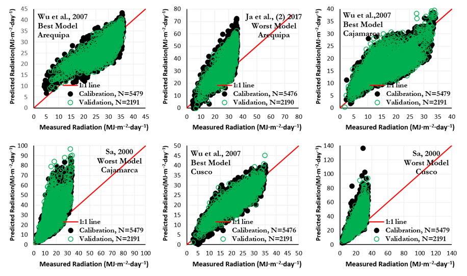
Atmosphere 12 00389 g001
Figure 2. Measured solar radiation versus values estimated by best and poorest empirical models in calibration and validation sets at all stations.
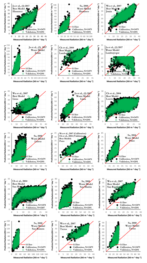
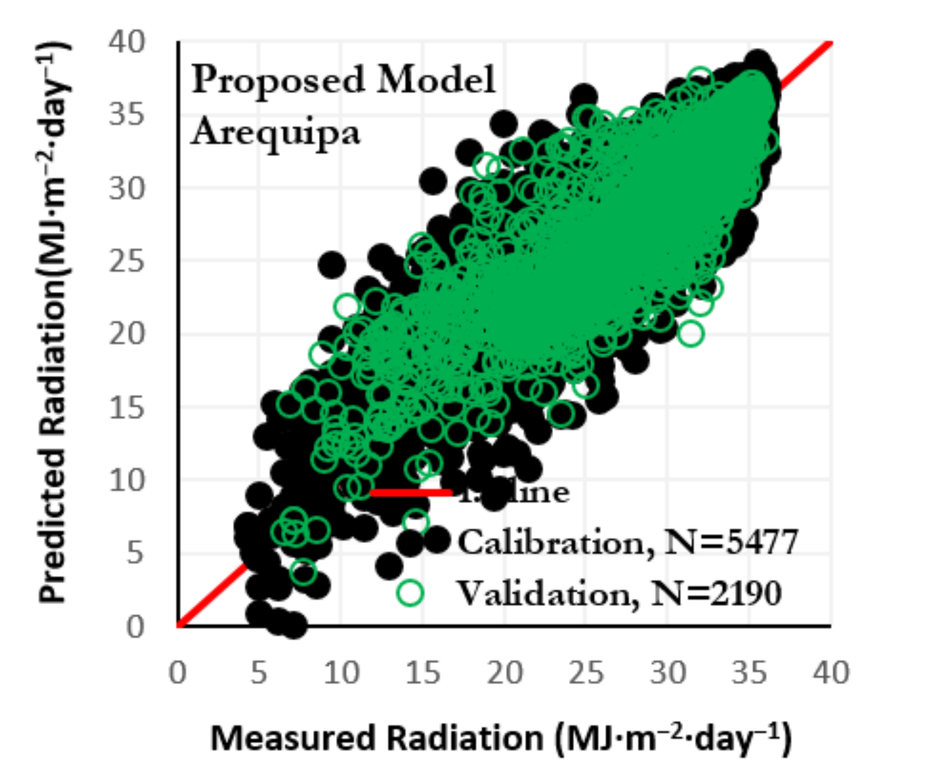
Atmosphere 12 00389 g002aAtmosphere 12 00389 g002bAtmosphere 12 00389 g002c
Figure 3. Solar radiation estimated by proposed model at Arequipa station versus measured values in calibration and validation sets.
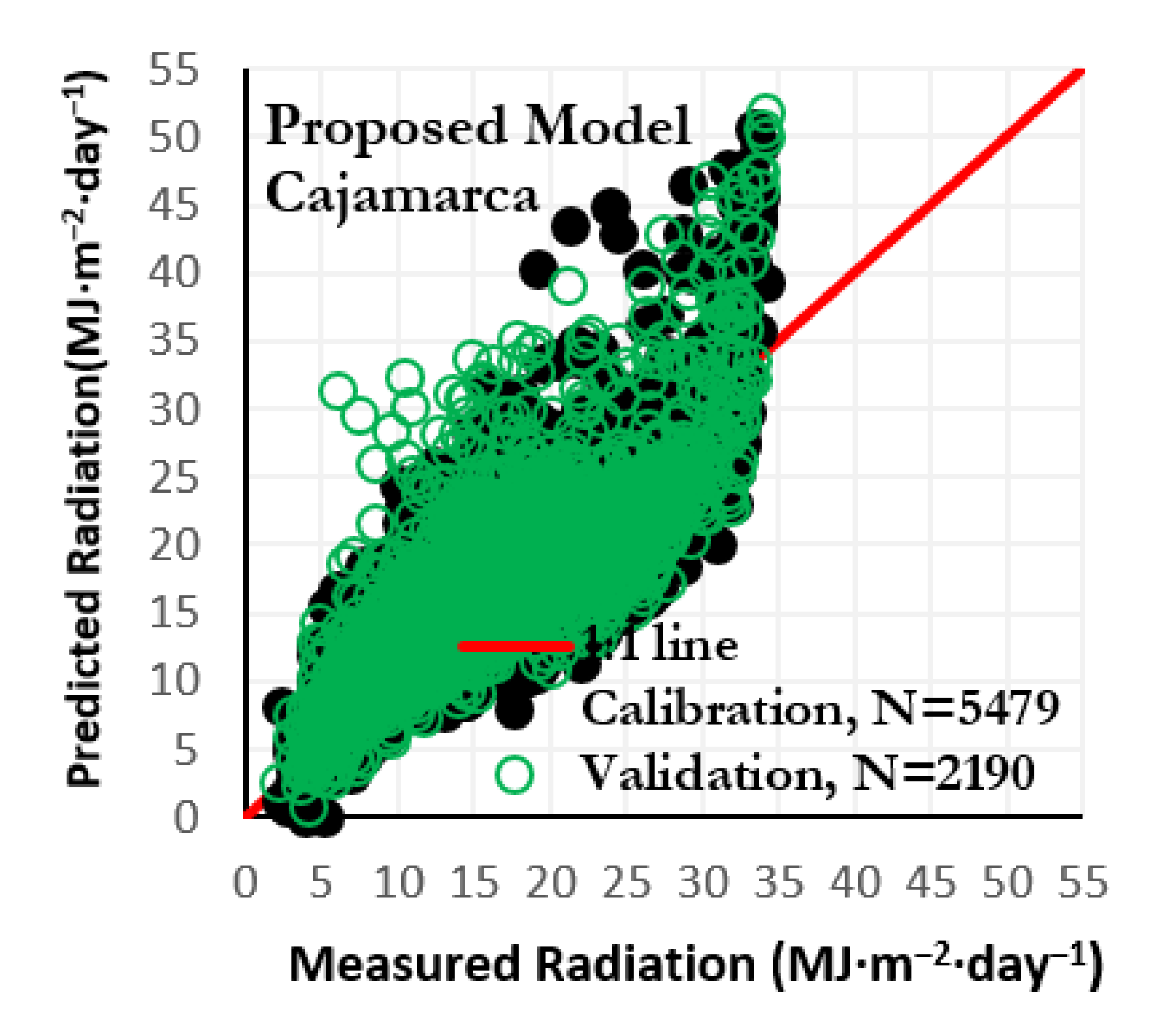
Atmosphere 12 00389 g003
Figure 4. Solar radiation estimated by proposed model at Cajamarca station versus measured values in calibration and validation sets.
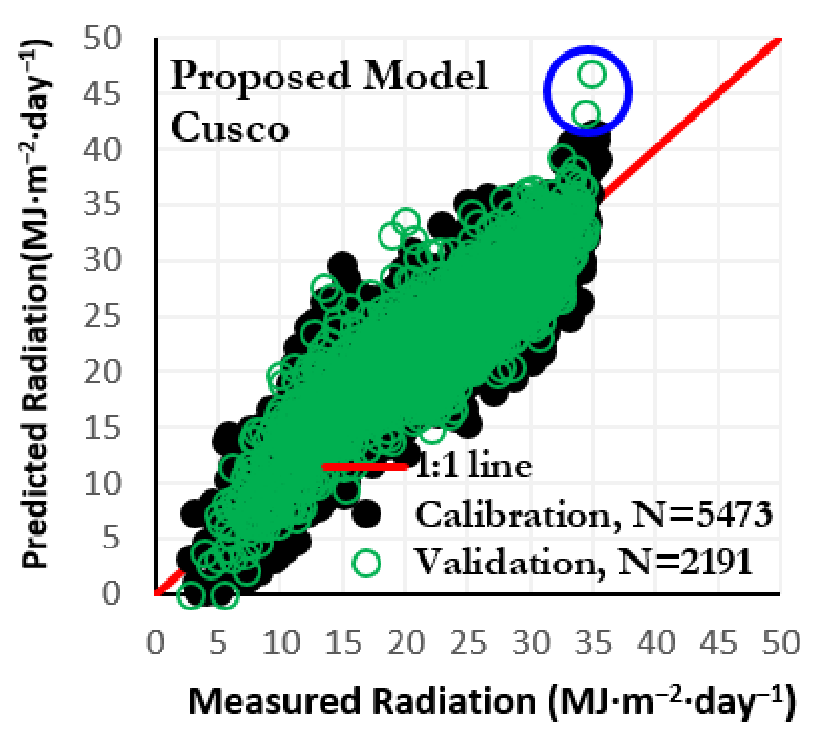
Atmosphere 12 00389 g004
Figure 5. Solar radiation estimated by proposed model at Cusco station versus measured values in calibration and validation sets.
Atmosphere 12 00389 g005
Figure 6. Solar radiation estimated by proposed model at Huanuco station versus measured values in calibration and validation sets.
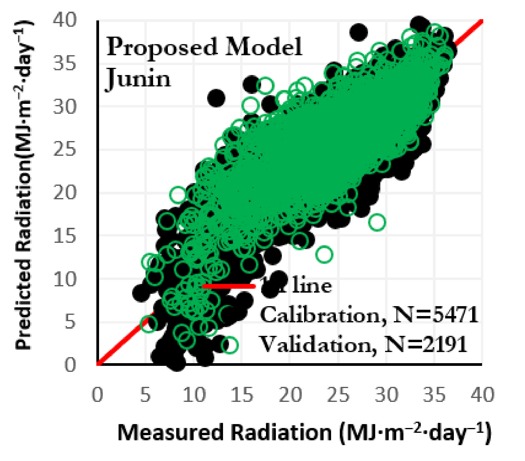
Atmosphere 12 00389 g006
Figure 7. Solar radiation estimated by proposed model at Junin station versus measured values in calibration and validation sets.
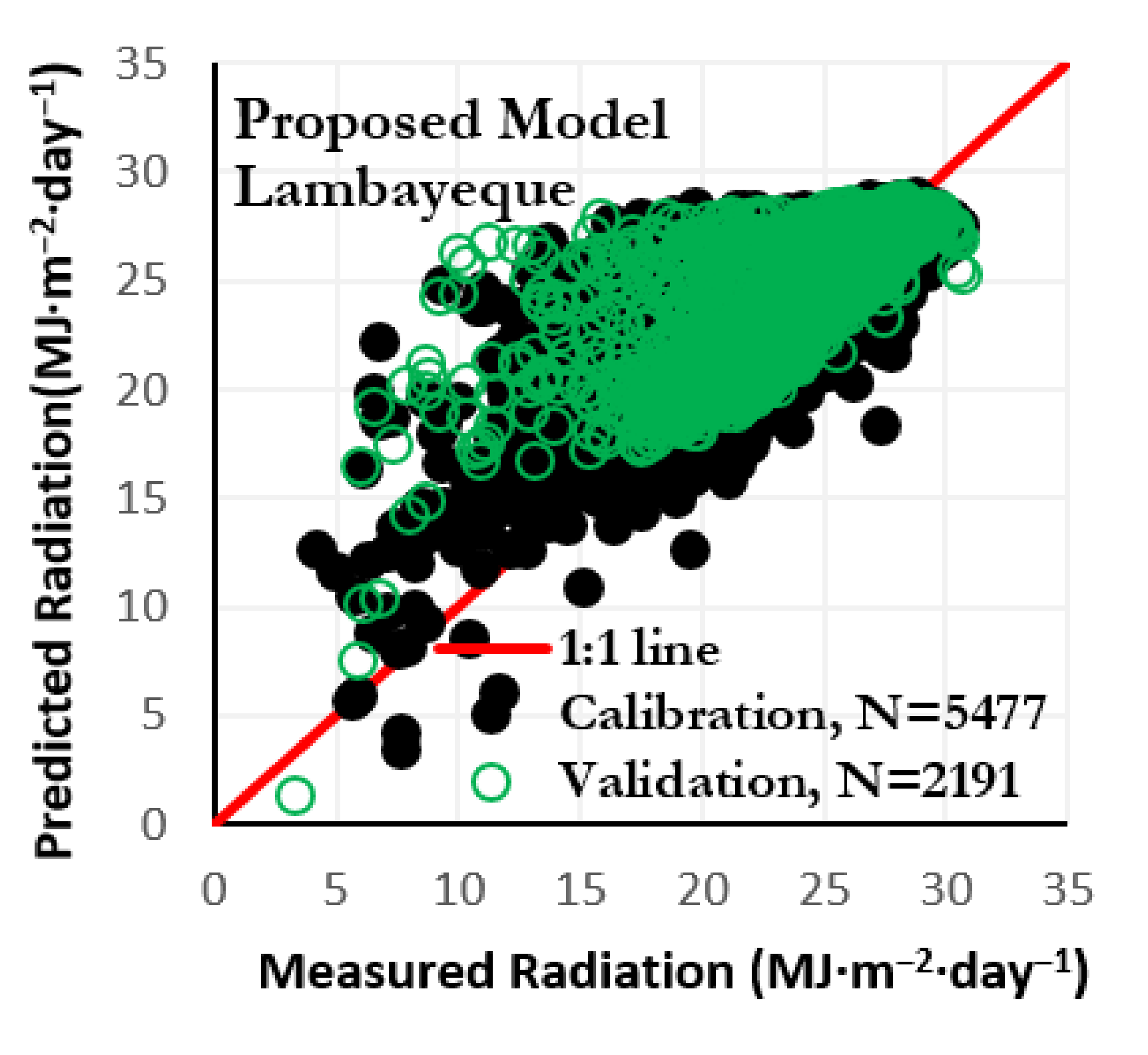
Atmosphere 12 00389 g007
Figure 8. Solar radiation estimated by proposed model at Lambayeque station versus measured values in calibration and validation sets.
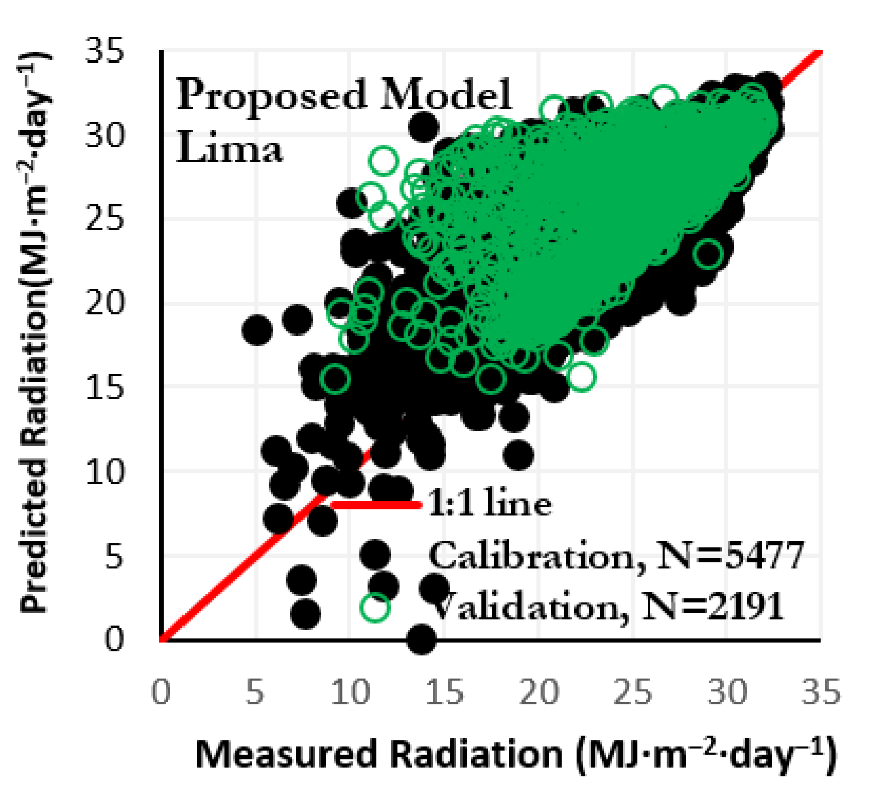
Atmosphere 12 00389 g008
Figure 9. Solar radiation estimated by proposed model at Lima station versus measured values in calibration and validation sets.
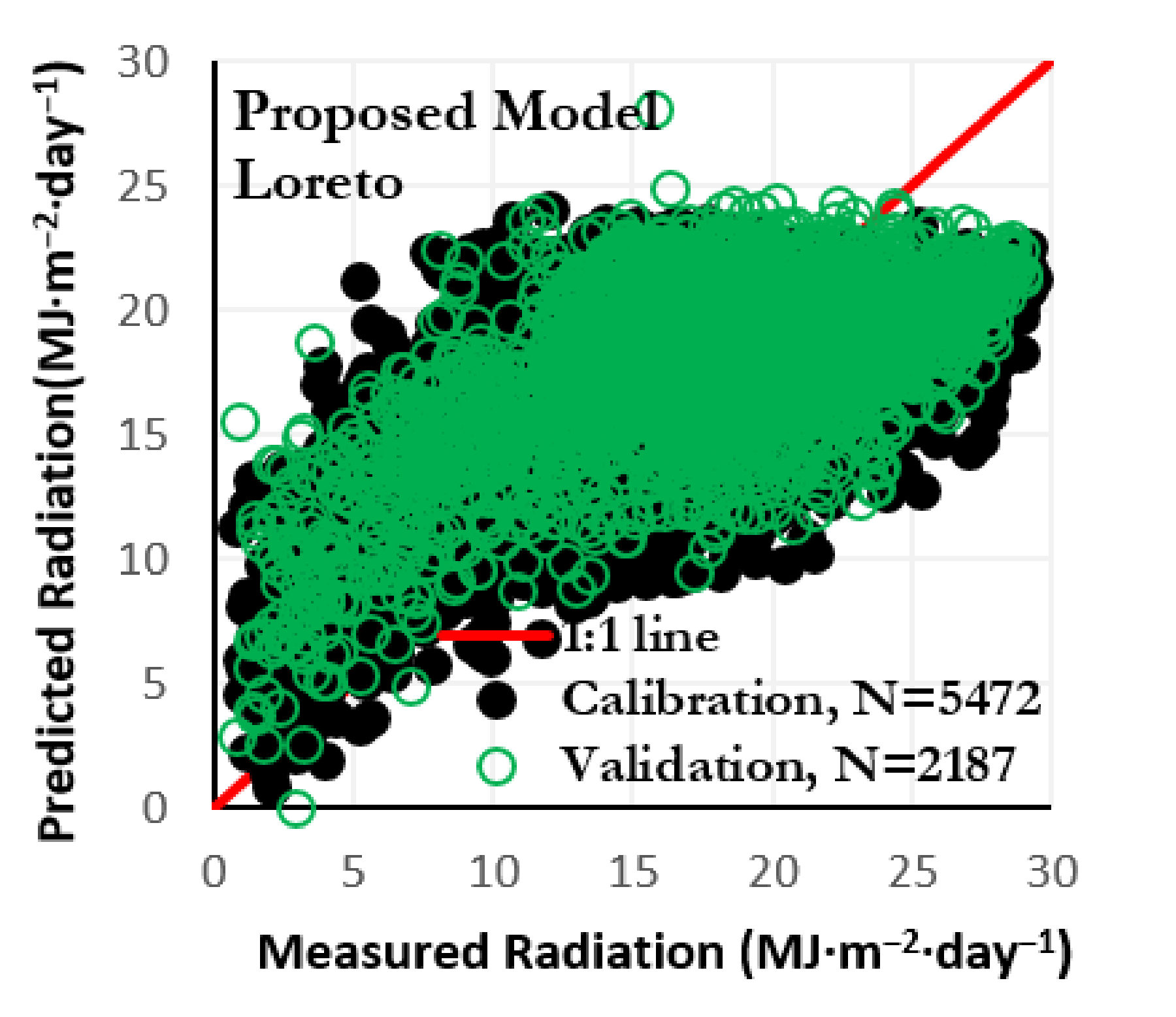
Atmosphere 12 00389 g009
Figure 10. Solar radiation estimated by proposed model at Loreto station versus measured values in calibration and validation sets.
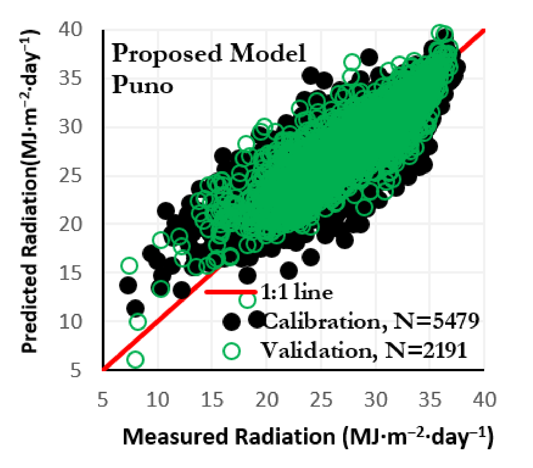
Atmosphere 12 00389 g010
Figure 11. Solar radiation estimated by proposed model at Puno station versus measured values in calibration and validation sets.
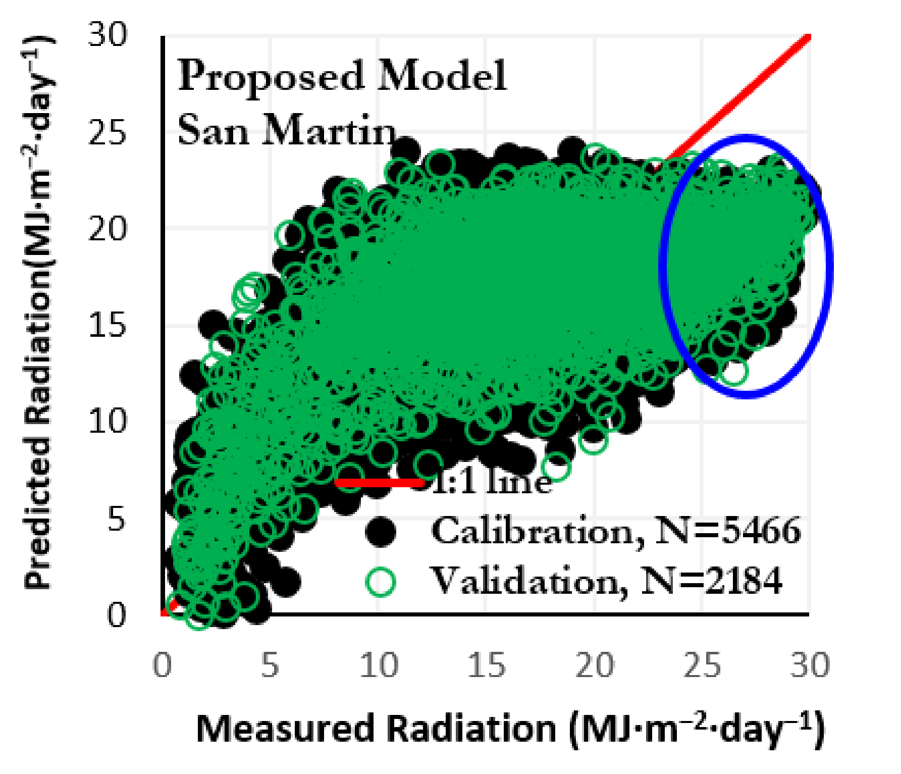
Atmosphere 12 00389 g011
Figure 12. Solar radiation estimated by proposed model at San Martin station versus measured values in calibration and validation sets.
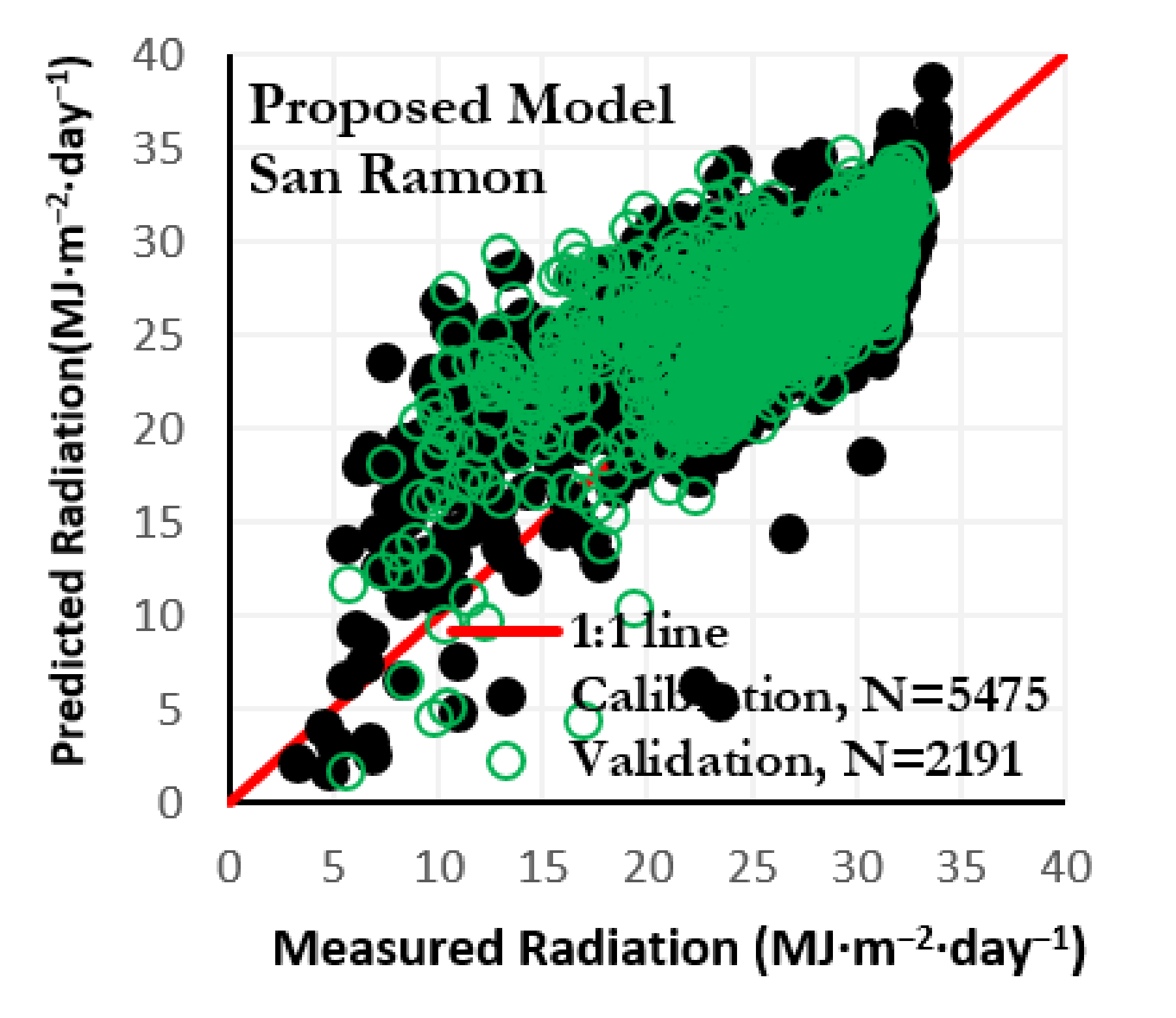
Atmosphere 12 00389 g012
Figure 13. Solar radiation estimated by proposed model at San Ramon station versus measured values in calibration and validation sets.
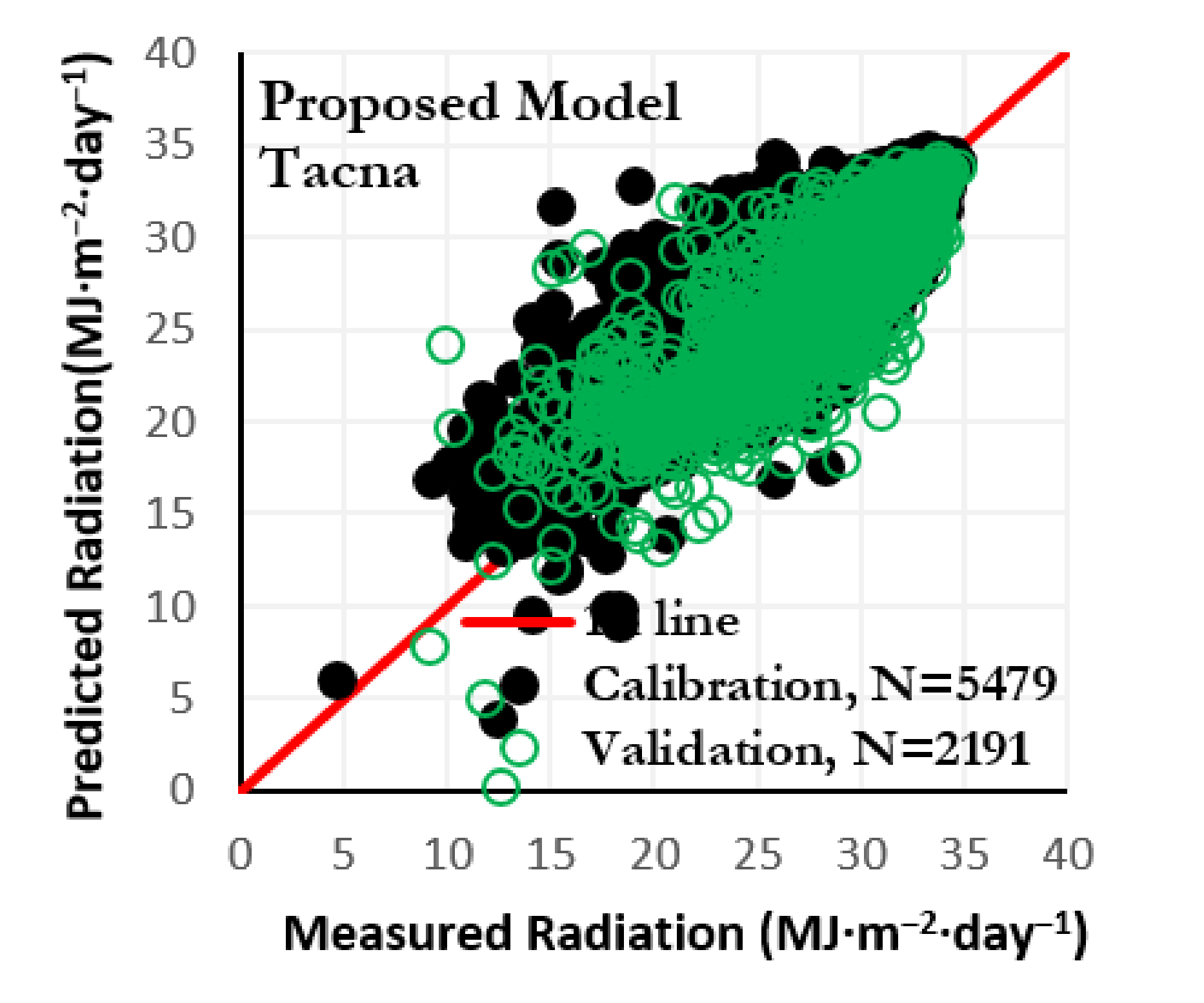
Atmosphere 12 00389 g013
Figure 14. Solar radiation estimated by proposed model at Tacna station versus measured values in calibration and validation sets.
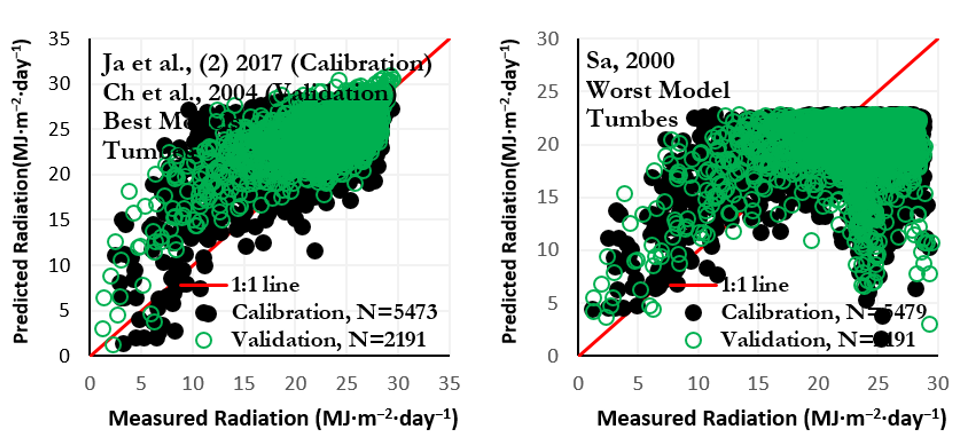
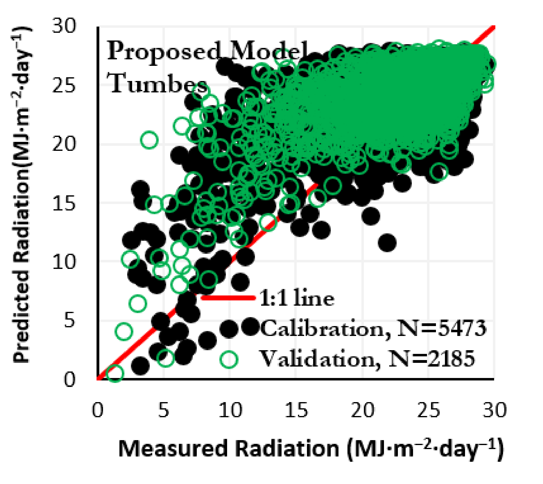
Atmosphere 12 00389 g014
Figure 15. Solar radiation estimated by proposed model at Tumbes station versus measured values in calibration and validation sets.
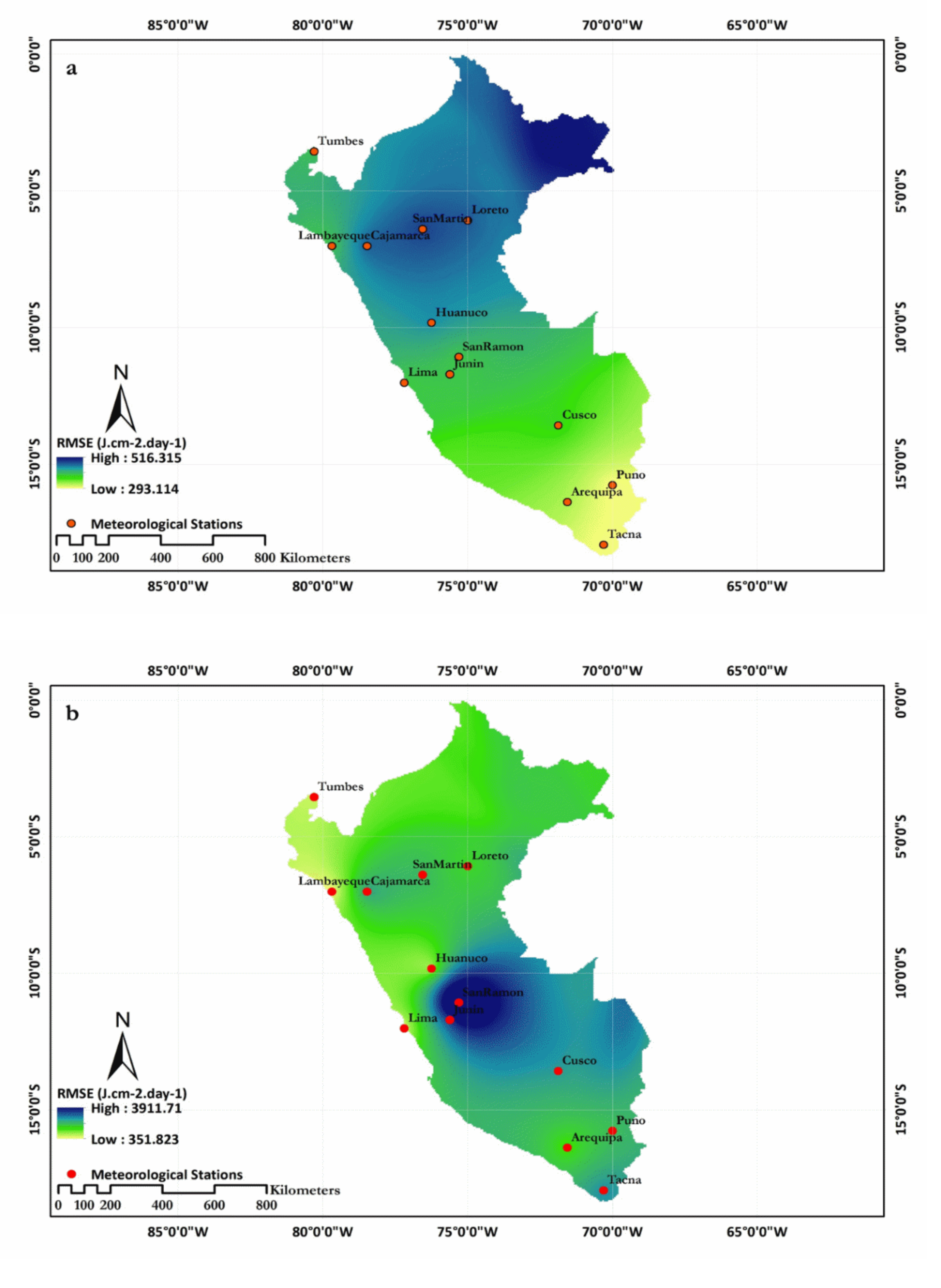
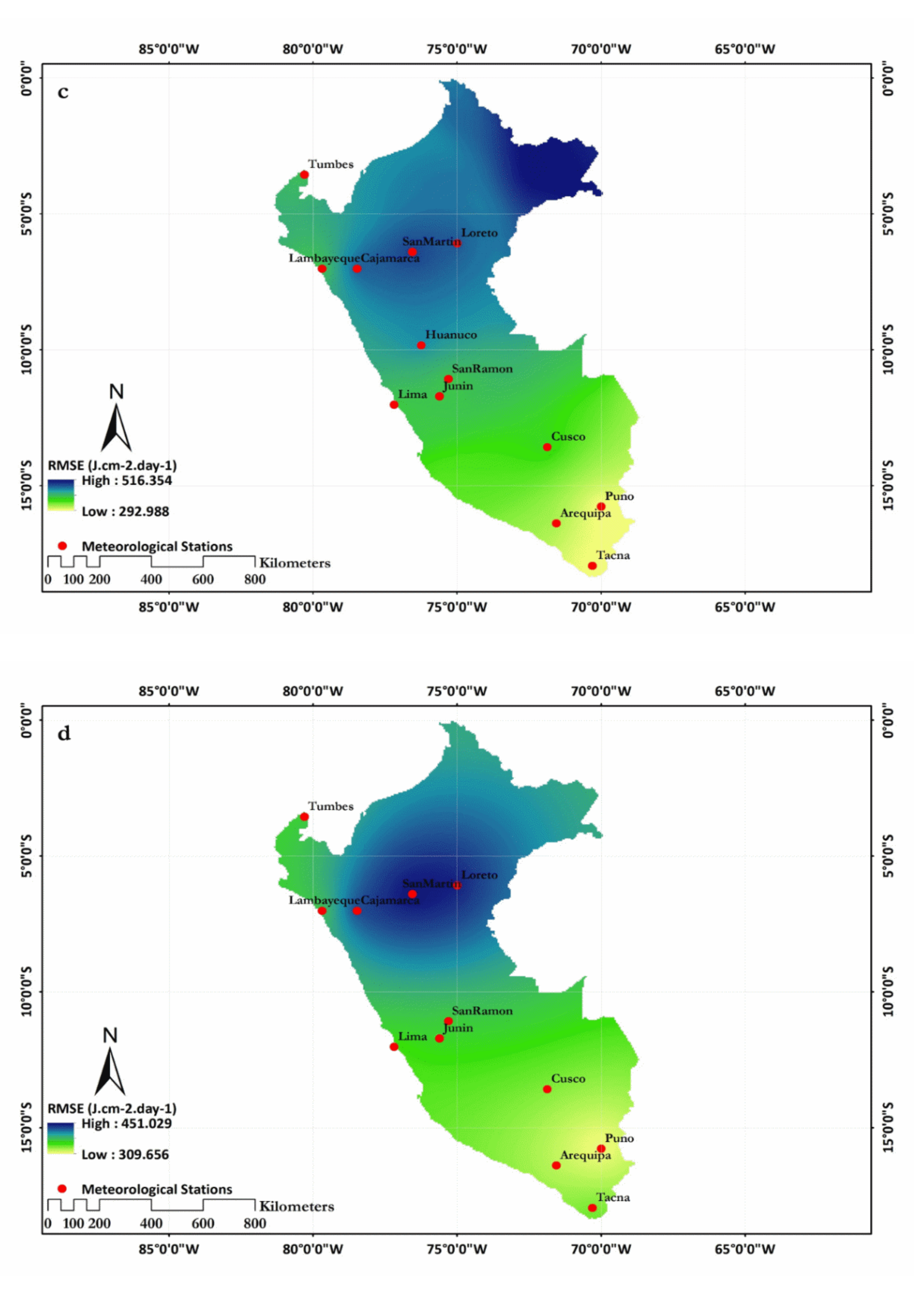
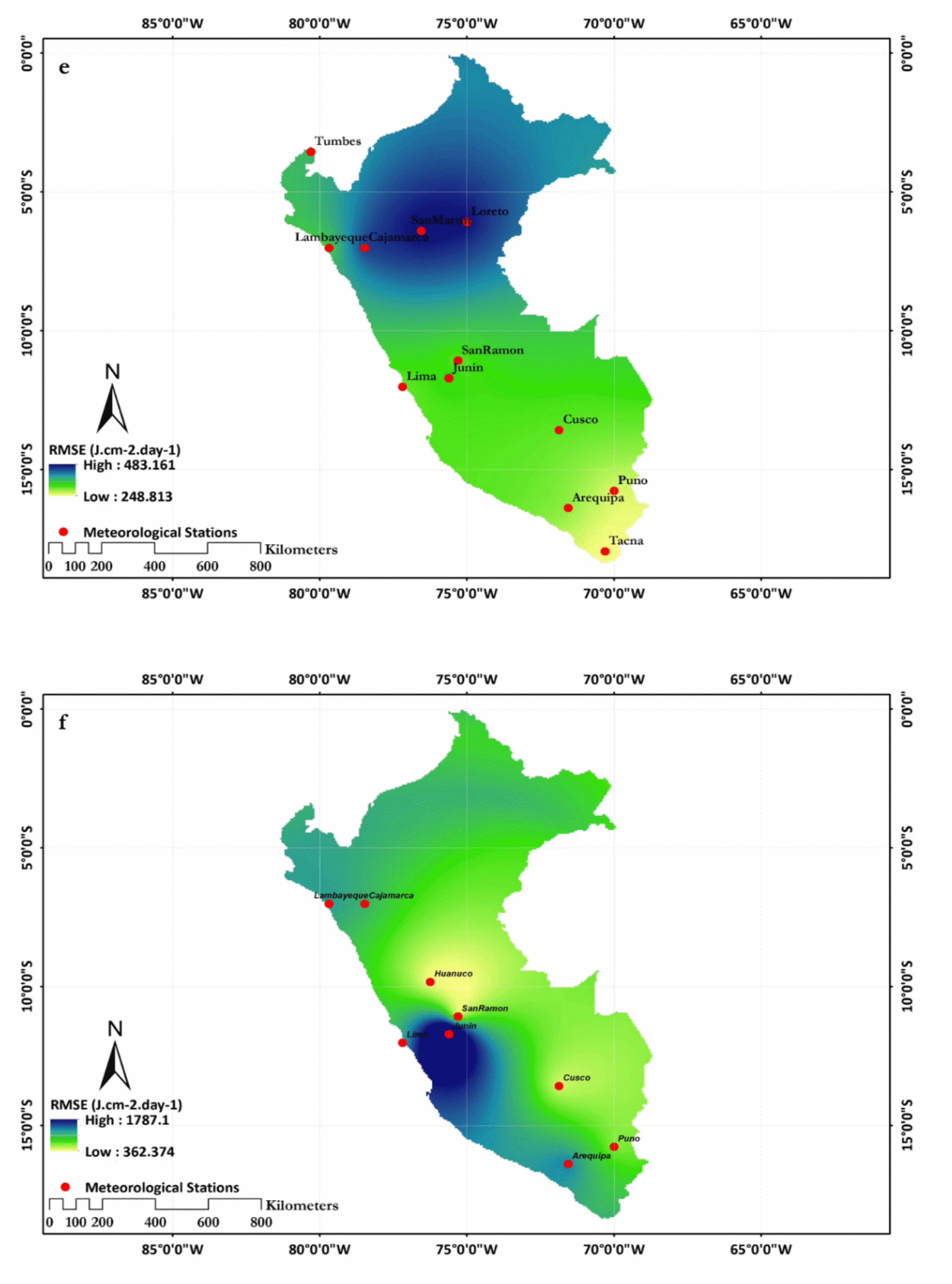
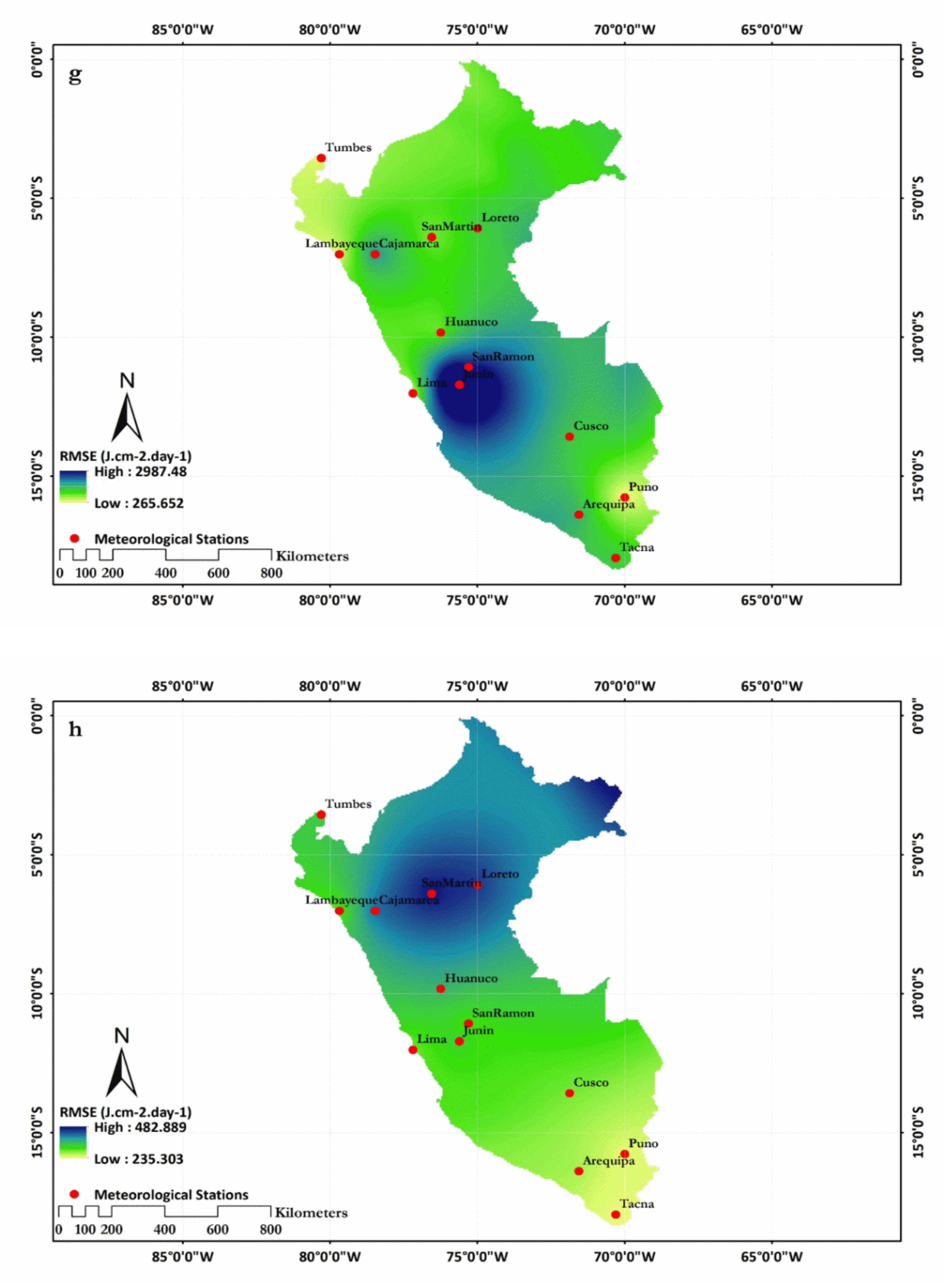
Atmosphere 12 00389 g015
Figure 16. Interpolated spatial distribution of error in solar radiation estimation at all stations using (a) Hargreaves-Samani [30] and (b) Samani [31] models (c) Annandale et al. [32] and (d) Chen et al. [33] models (e) Wu et al. [36] and (f) Jahani et al. 1 [2] models (g) Jahani et al. 2 [2] and (h) proposed models.
Atmosphere 12 00389 g016aAtmosphere 12 00389 g016bAtmosphere 12 00389 g016cAtmosphere 12 00389 g016d
Table 1. Statistical indices for climatic parameters recorded in 13 Peruvian meteorological stations over the time period covered in this study.
ParameterCVSDMeanMaxMin
Min temperature (°C)0.88.4110.4528.9−17.3
Max temperature (°C)0.32721.9642.70.9
Altitude (m)0.861749.492026499017
Relative humidity (%)0.2315.968.1994
Extraterrestrial Radiation (MJ·m−2·day−1)0.194.2135.4741.7125.07
Solar Radiation (MJ·m−2·day−1)0.36.7722.2537.440.65
SD: standard deviation, CV: coefficient of variation.
Table 2. Empirical models used for estimating solar radiation.
Empirical ModelEquation
Hargreaves-Samani [30] R s = R a a Δ T 0.5
Samani [31] R s = R a C 1 Δ T 2.5 + C 2 Δ T 1.5 + C 3 Δ T 0.5
Annandale et al. [32] R s = R a d 1 + 2.7 * 10 6 Z Δ T 0.5
Chen et al. [33] R s = R a e 1 + e 2 l n Δ T
Wu et al. [36] R s = R a i 1 + i 2 Δ T 0.5 + i 3 T m e a n + i 4 P t
Jahani et al. 1 [2] R s = R a β 1 + β 2 Δ T + β 3 Δ T 2 + β 4 Δ T 3
Jahani et al. 2 [2] R s = R a γ 1 + γ 2 Δ T 0.5 + γ 3 Δ T 1.5 + γ 4 Δ T 2.5
Table 3. Calibrated coefficients for the best empirical models for each station.
StationBest ModelModel Coefficients
TumbesJahani et al. 2 (2017)γ1 = −0.827, γ2 = 0.644, γ3 = −0.017, γ4 = 0.000063
CuscoWu et al. (2007)i1 = −0.456, i2 = 0.289, i3 = 0.024, i4 = −0.059
ArequipaWu et al. (2007)i1 = −0.223, i2 = 0.243, i3 = 0.015, i4 = −0.083
LimaWu et al. (2007)i1 = 0.444, i2 = 0.165, i3 = −0.008, i4 = −0.083
LorettoChen et al. (2004)e1 = 0.022, e2 = 0.194
SanRamonWu et al. (2007)i1 = −0.021, i2 = 0.15, i3 = 0.01, i4 = −0.18
PunoWu et al. (2007)i1 = 0.136, i2 = 0.156, i3 = 0.004, i4 = −0.06
TacnaWu et al. (2007)i1 = 0.221, i2 = 0.131, i3 = 0.004, i4 = −0.075
SanMartinChen et al. (2004)e1 = −0.031, e2 = 0.215
LambayequeChen et al. (2004)e1 = 0.215, e2 = 0.238
JuninWu et al. (2007)i1 = −0.148, i2 = 0.234, i3 = 0.006, i4 = −0.078
CajamarcaWu et al. (2007)i1 = 0.044, i2 = 0.223, i3 = −0.015, i4 = −0.122
HuanucoJahani et al. 1 (2017)β1 = −0.002, β1 = 0.05, β1 = 0.002, β1 = −0.000093
Table 4. Root mean square errors (RMSEs) (J·cm−2·day−1) of solar radiation estimated by empirical models in selected meteorological stations (calibration set).
ModelsStations
TumbesCuscoArequipaLimaLorettoSanRamonPunoTacnaSanMartinLambayequeJuninCajamarcaHuanuco
Hg-Sa313.3400.9385.7299504.9310.1261.5242.2525.6252.5364.1524.6481.3
Sa510.21840.5998.4375.21464.63969.51250.71975.11660285.22029.31475.9697.2
An313.3401.1385.8298.5505310.1261.5241.5525.6252.5364.1524.4481.9
Chen302345.3339.7286.1489.7302.1257221.6514.4233.6325.1497-
Wu310.6307.7338.3274501239.7253.7220520.1236.8308.2473.8-
Ja1-400.5901.7658.3-413.2534.8--722.61553.8691.4371.8
Ja2 293980.91026.4296.310871738.8269.5972.1589.1282.926791087645.9
The best values at each station are marked in bold. Hg-Sa (Hargreaves-Samani, [30] 1982), Sa (Samani, [31], An (Annandale et al. [32]), Chen (Chen et al. [33]), Wu (Wu et al. [36]), Ja1 (Jahani et al. [2], first model), and Ja2 (Jahani et al. [2], second model).
Table 5. RMSEs (J·cm−2·day−1) of solar radiation estimated by empirical models in selected meteorological stations (validation set).
ModelsStations
TumbesCuscoArequipaLimaLoretoSanRamonPunoTacnaSan MartinLambayequeJuninCajamarcaHuanuco
Hg-Sa349.1412.1336.7346.6500.6351.1242.4269.6530.6307.6398.8551478.9
Sa546.417601025.6480.61181.63958.41417.51845.21479.6338.62300.71666.7727.6
An 349.2412.6337.5345.1500.5351.9242.2270.7530.3307.6398.9551.2479.7
Chen 336.6345.3315.6324.9488343.9236.3370.5517.6275378.6531.9-
Wu 351.1317.6314.8291.9508272.8246.4227.1517.7281.9364.3505.8-
Ja1 -422.5919.5794.9-412.7539.1--850.31801.8773.5367.1
Ja2 337.2924.81047.9371.5866.91764262.1900.8616.9315.23005.71233.7670.1
The best values at each station are marked in bold.
Table 6. New models proposed for estimating solar radiation in each station.
StationProposed Model
Arequipa R s = R a 0.61 0.16 R H 0.905 t 1 0.352 l n T m e a n 0.007 P r e + 0.699 l n Δ T
Cajamarca R s = R a 1.137 1.079 R H 0.013 T m e a n 0.002 P r e + 0.139 l n Δ T
Cusco R s = R a 0.162 0.673 R H + 0.366 t 1 + 0.04 T m e a n 0.001 P r e + 0.152 l n Δ T
Huanuco R s = R a 0.293 0.496 R H + 1.412 t 1 + 0.088 T m e a n 0.001 P r e 0.293 l n Δ T
Junin R s = R a 0.045 0.236 R H + 0.006 t 1 0.011 P r e + 0.35 l n Δ T
Lambayeque R s = R a 1.572 + 0.057 R H 2.164 t 1 0.536 l n T m e a n 0.005 P r e + 0.683 l n Δ T
Lima R s = R a 2.834 0.356 R H 2.766 t 1 0.871 l n T m e a n 0.06 P r e + 0.816 l n Δ T
Loreto R s = R a 0.588 + 0.242 R H 0.4 t 1 + 0.068 l n T m e a n + 0.001 P r e + 0.337 l n Δ T
Puno R s = R a 0.052 0.157 R H + 0.009 t 1 + 0.002 T m e a n 0.005 P r e + 0.275 l n Δ T
San Martin R s = R a 1.027 + 0.159 R H 0.257 t 1 + 0.245 l n T m e a n + 0.001 P r e + 0.295 l n Δ T
San Ramon R s = R a 0.197 0.185 R H + 0.513 t 1 + 0.024 T m e a n 0.036 P r e + 0.103 l n Δ T
Tacna R s = R a 1.355 0.076 R H 1.508 t 1 0.582 l n T m e a n 0.017 P r e + 0.76 l n Δ T
Tumbes R s = R a 1.076 + 0.058 l n R H 0.472 t 2 0.507 l n T m e a n + 0.533 l n Δ T
Table 7. RMSEs (J·cm−2·day−1) and number of data points (proposed model) in under- and overestimation sets for measured solar radiation values lower or higher than 20 MJ·m−2·day−1 in validation set.
Measured Rs Lower than 20 MJ·m−2·day−1Measured Rs Higher than 20 MJ·m−2·day−1
Data SetUnder-EstimatedOverestimatedUnderestimatedOverestimated
validation284.4 (n = 27)559.6 (n = 197)236.9 (n = 1085)234.5 (n = 881)
Table 8. RMSE values (J·cm−2·day−1) and number of data points in under- and overestimation sets for measured solar radiation values lower or higher than mean (Rs)mea in calibration and validation sets.
Measured Rs Lower than Mean (Rs)meaMeasured Rs Higher than Mean (Rs)mea
Data SetUnderestimatedOverestimatedUnderestimatedOverestimated
calibration189.9 (n = 675)405.5 (n = 2116)371.9 (n = 2012)453.3 (n = 676)
validation188.2 (n = 200)487.6 (n = 946)384.3 (n = 747)598.8 (n = 297)
Table 9. RMSE values (J·cm−2·day−1) and number of data points belonging to under- and overestimation sets in calibration and validation phases using proposed model.
Data SetCalibrationValidation
underestimated242.5 (n = 3061)244 (n = 1170)
overestimated324 (n = 2412)339.5 (n = 1021)
Table 10. RMSE values (J·cm−2·day−1) and number of data points belonging to each group separated by a threshold value (mean of measured solar radiation): lower and higher than the mentioned threshold in calibration and validation sets.
Data SetCalibrationValidation
Rs < Mean (Rs)mea326 (n = 2224)345.4 (n = 867)
Rs > Mean (Rs)mea246.1 (n = 3249)251.7 (n = 1324)
Table 11. RMSE values (J·cm−2·day−1) and number of data points belonging to under- and overestimation sets for measured solar radiation less or higher than mean (Rs)mea in calibration and validation phases using proposed model.
Measured Rs Lower than Mean (Rs)meaMeasured Rs Higher than Mean (Rs)mea
Data SetUnderestimatedOverestimatedUnderestimatedOverestimated
calibration176.9 (n = 865)353.8 (n = 1970)357.3 (n = 1716)327.5 (n = 902)
validation174.3 (n = 248)400 (n = 842)333.3 (n = 644)439.6 (n = 457)
Table 12. RMSE values (J·cm−2·day−1) and number of data points belonging to under- and overestimation sets for measured solar radiation less or higher than mean (Rs)mea in calibration and validation phases using proposed model.
Measured Rs Lower than Mean (Rs)meaMeasured Rs Higher than Mean (Rs)mea
Data SetUnderestimatedOverestimatedTotal Data SetUnderestimatedOverestimatedTotal Data Set
calibration239.6444.2370.8240.2194.5227.5
(n = 1112)(n = 1489)(n = 2601)(n = 2010)(n = 860)(n = 2870)
validation225.8524.7457219.9243.4229.3
(n = 292)(n = 694)(n = 986)(n = 736)(n = 469)(n = 1205)
Table 13. RMSE values (J·cm−2·day−1) and number of data points belonging to under- and overestimation sets in three defined intervals of measured solar radiation (MJ·m−2·day−1) for calibration and validation phases using proposed model.
CalibrationValidation
Data SetRs < 1010 ≤ Rs < 20Rs ≥ 20Rs < 1010 ≤ Rs < 20Rs ≥ 20
underpredicted379 (n = 2)139.2 (n = 221)144.8 (n = 3180)184 (n = 1)60.62 (n = 29)113.3 (n = 1109)
overpredicted750.8 (n = 35)462.7 (n = 565)181.1 (n = 1474)1088.5 (n = 16)559 (n = 264)200.3 (n = 772)
Table 14. RMSE values (J·cm−2·day−1) and number of data points belonging to under- and overestimation sets in three defined intervals of measured solar radiation (MJ·m−2·day−1) for calibration and validation phases using proposed model.
CalibrationValidation
Data SetRs < 1515 ≤ Rs < 25Rs ≥ 25Rs < 1515 ≤ Rs < 25Rs ≥ 25
underestimated534.4 (n = 17)151.1 (n = 1618)159.7 (n = 1859)-101.9 (n = 586)95.7 (n = 663)
(n = 0)
overestimated677.6 (n = 141)371.9 (n = 1163)140 (n = 679)1047.2 (n = 28)469.7 (n = 565)180.6 (n = 349)
Table 15. RMSE values (J·cm−2·day−1) and number of data points belonging to under- and overestimation sets in three defined intervals of measured solar radiation (MJ·m−2·day−1) for calibration and validation phases using proposed model.
CalibrationValidation
Data SetRs < 1010 ≤ Rs < 20Rs ≥ 20Rs < 1010 ≤ Rs < 20Rs ≥ 20
underestimated143.5 (n = 34)290.7 (n = 1024)548.3 (n = 1670)207.6 (n = 3)266.2 (n = 342)501.9
(n = 699)
overestimated673.3 (n = 691)426.8 (n = 1989)103 (n = 64)698.9 (n = 295)416.9 (n = 797)140.4 (n = 51)
Table 16. RMSE values (J·cm−2·day−1) and number of data points belonging to under- and overestimation sets for measured solar radiation less or higher than mean (Rs)mea in calibration and validation phases using proposed model.
Measured Rs Lower than Mean (Rs)meaMeasured Rs Higher than Mean (Rs)mea
Data SetUnderpredictedOverpredictedUnderpredictedOverpredicted
calibration145.6 (n = 1308)321.4 (n = 1577)252.7 (n = 1834)181.5 (n = 760)
validation119.9 (n = 452)321.8 (n = 689)208.4 (n = 585)192.2 (n = 465)
Table 17. RMSE values (J·cm−2·day−1) and number of data points belonging to under- and overestimation sets in three defined intervals of measured solar radiation (MJ·m−2·day−1) for calibration and validation phases using proposed model.
CalibrationValidation
Data SetRs < 1515 ≤ Rs < 30Rs ≥ 30Rs < 1515 ≤ Rs < 30Rs ≥ 30
underpredicted-175.9 (n = 1981)268.2 (n = 1166)181.8140 (n = 682)228.7 (n = 354)
(n = 0)(n = 1)
overpredicted601.8 (n = 49)288 (n = 1990)131.2 (n = 298)642.4 (n = 16)285 (n = 958)151
(n = 180)
Table 18. RMSE values (J·cm−2·day−1) and number of data points belonging to under- and overestimation sets for measured solar radiation less or higher than mean (Rs)mea in calibration and validation phases using proposed model.
Measured Rs Lower than Mean (Rs)meaMeasured Rs Higher than Mean (Rs)mea
Data SetUnderestimatedOverestimatedUnderestimatedOverestimated
calibration214.3 (n = 318)524.7 (n = 2312)563.9 (n = 2220)221.7 (n = 616)
validation196.9 (n = 118)529 (n = 938)551.4 (n = 953)221 (n = 175)
Table 19. RMSE values (J·cm−2·day−1) and number of data points belonging to under- and overestimation sets in three defined intervals of measured solar radiation (MJ·m−2·day−1) for calibration and validation phases using proposed model.
CalibrationValidation
Data SetRs < 1010 ≤ Rs < 20Rs ≥ 20Rs < 1010 ≤ Rs < 20Rs ≥ 20
underestimated169.7310.5 (n = 919)633 (n = 1574)135.8279.8 (n = 370)620.3 (n = 689)
(n = 45)(n = 12)
overestimated632 (n = 741)417.3 (n = 2126)102.7 (n = 61)645.4 (n = 345)411.9 (n = 749)107.2
(n = 19)
Table 20. RMSE values (J·cm−2·day−1) and number of data points belonging to under- and overestimation sets in two defined intervals of measured solar radiation (MJ·m−2·day−1) for calibration and validation phases using proposed model.
CalibrationValidation
Data SetRs < 20Rs ≥ 20Rs < 20Rs ≥ 20
underestimated263.3 (n = 20)180.5 (n = 3513)469.1 (n = 15)167.5 (n = 1410)
overestimated737.5 (n = 277)207.5 (n = 1665)836.6 (n = 142)241.7 (n = 624)
Table 21. RMSE values (J·cm−2·day−1) and number of data points belonging to under- and overestimation sets in three defined intervals of measured solar radiation (MJ·m−2·day−1) for calibration and validation phases using proposed model.
CalibrationValidation
Data SetRs < 1515 ≤ Rs < 25Rs ≥ 25Rs < 1515 ≤ Rs < 25Rs ≥ 25
underestimated552.2101.4 (n = 1453)188.2 (n = 1854)715.7134.9 (n = 725)236.9 (n = 932)
(n = 3)(n = 4)
overestimated583.2 (n = 60)294 (n = 1111)166.6 (n = 998)706.5 (n = 18)318.4 (n = 251)165.3
(n = 261)
Table 22. RMSE values (J·cm−2·day−1) and number of data points belonging to under- and overestimation sets in two defined intervals of measured solar radiation (MJ·m−2·day−1) for calibration and validation phases using proposed model.
CalibrationValidation
Data SetRs < 20Rs ≥ 20Rs < 20Rs ≥ 20
underestimated239.4 (n = 38)200.1 (n = 3442)146 (n = 8)167.2 (n = 1067)
overestimated649.2 (n = 608)198.7 (n = 1385)703.4 (n = 337)222.1 (n = 773)
Table 23. RMSEs (J·cm−2·day−1) of the proposed models and percentage of RMSE reduction by proposed models compared to best, poorest, and average results of empirical models in each of the 13 selected stations at calibration (validation) set.
Percentage of RMSE Reduction Compared to the Average of All Empirical ModelsPercentage of RMSE Reduction Compared to the Poorest-Performing Empirical ModelPercentage of RMSE Reduction Compared to the Best Empirical ModelRMSE (J·cm−2·day−1)Station
53 (54.2)71.4 (73.2)13.2 (10.7)293.7 (281.2)Arequipa
49.6 (45.5)74.3 (72.8)19.9 (10.5)379.6 (452.7)Cajamarca
57.9 (55.5)84.7 (83.4)8.6 (7.9)281.3 (292.4)Cusco
38.6 (31.8)52.8 (44.6)11.6 (1.1)328.8 (371.3)Huanuco
72 (71.6)88.6 (88.3)1.3 (3.8)304.2 (350.6)Junin
32.6 (32.3)69.8 (69.6)6.7 (5.9)218 (258.8)Lambayeque
31.1 (32.2)62.8 (64)10.7 (2.1)244.7 (285.8)Lima
36.6 (30.2)67.2 (60.2)1.8 (3.6)480.9 (470.5)Loreto
44.1 (48.5)80.3 (83.5)2.8 (0.8)246.5 (234.4)Puno
30.3 (27.2)69.7 (65.6)2 (1.7)503.8 (508.8)San Martin
76.1 (73.2)93.7 (92.8)3.7 (4.7)248.5 (285.6)San Ramon
68.6 (65.5)89.7 (87.9)7.8 (1.7)202.9 (223.2)Tacna
15.7 (13.3)43.7 (40)2 (2.6)287 (327.8)Tumbes
Publisher’s Note: MDPI stays neutral with regard to jurisdictional claims in published maps and institutional affiliations.

