Article

GIS-Based Approach to Spatio-Temporal Interpolation of Atmospheric CO2 Concentrations in Limited Monitoring Dataset

1
Faculty of Environmental Engineering, Wroclaw University of Science and Technology, Plac Grunwaldzki 13, 50-377 Wroclaw, Poland
2
Faculty of Earth Science and Environmental Management, University of Wroclaw, Cybulskiego 32, 50-205 Wroclaw, Poland
3
Faculty of Geoengineering, Mining and Geology, Wroclaw University of Science and Technology, Na Grobli 15, 50-421 Wroclaw, Poland
*
Author to whom correspondence should be addressed.
Atmosphere 2021, 12(3), 384; https://doi.org/10.3390/atmos12030384
Submission received: 11 February 2021 / Revised: 4 March 2021 / Accepted: 8 March 2021 / Published: 15 March 2021

Abstract

:
Understanding the magnitude and distribution of the mixes of the near-ground carbon dioxide (CO2) components spatially (related to the surface characteristics) and temporally (over seasonal timescales) is critical to evaluating present and future climate impacts. Thus, the application of in situ measurement approaches, combined with the spatial interpolation methods, will help to explore variations in source contribution to the total CO2 mixing ratios in the urban atmosphere. This study presents the spatial characteristic and temporal trend of atmospheric CO2 levels observed within the city of Wroclaw, Poland for the July 2017–August 2018 period. The seasonal variability of atmospheric CO2 around the city was directly measured at the selected sites using flask sampling with a Picarro G2201-I Cavity Ring-Down Spectroscopy (CRDS) technique. The current work aimed at determining the accuracy of the interpolation techniques and adjusting the interpolation parameters for estimating the magnitude of CO2 time series/seasonal variability in terms of limited observations during the vegetation and non-vegetation periods. The objective was to evaluate how different interpolation methods will affect the assessment of air pollutant levels in the urban environment and identify the optimal sampling strategy. The study discusses the schemes for optimization of the interpolation results that may be adopted in areas where no observations are available, which is based on the kriging error predictions for an appropriate spatial density of measurement locations. Finally, the interpolation results were extended regarding the average prediction bias by exploring additional experimental configurations and introducing the limitation of the future sampling strategy on the seasonal representation of the CO2 levels in the urban area.

1. Introduction

Atmospheric greenhouse gas (GHG) mixing ratio is strongly influenced by multiple human-induced and natural factors. The rising CO2 concentration in the atmosphere is a direct consequence of human activities, including a contribution of fossil fuel-derived emissions into the atmosphere and effects of land-use changes, etc. [1,2,3]. In addition, natural impacts through gas fluxes in ecosystems, carbon uptake and release from soils and sequestration by live vegetation, are also an important part of the terrestrial carbon cycle [4,5,6,7]. Evaluation of the urban carbon cycle, due to the mix of anthropogenic and natural emission effects, is often difficult and shows a greater number of potential uncertainties than in a wider spatial resolution. The accuracy of air quality studies depends on the precision of criteria that are estimated for a certain region meteorological fields and category of emission origins. At the present, the concentration of GHGs is mainly estimated by the measurements from nearest stations or single discrete observations. In practice, ground-based observations include a small number of sampling points in a limited spatial resolution. Datasets gathered in air pollution monitoring are often not complete in certain locations and contain missing value points. As a result, very little is known about the spatio-temporal variation of GHGs at an urban scale.
Given a large amount of daily CO2 variations in the urban environment, the attempt to spatial predictions of air pollution is appropriate [4,5,8]. The overall spatial patterns and the temporal evolution of the average concentration fields (pollution maps) derived from the field measurements with various weight factors (e.g., various meteorological conditions, terrain elevation, etc.) can provide realistic information on air quality in the unmeasured locations. Time information about the typical spatial patterns should also be noted to adequately represent the temporal effects of emission drivers (given emission sources, traffic intensity). The seasonal average CO2 concentration map in particular is assumed to be reasonable to underline the temporal processes of the fine-scale spatial variability of GHG reduction targets in the urban areas.
The problem of filling data gaps in monitoring measure series can be solved by taking the pollutant distribution trend and interpolating the missing data from surrounding values. Building geostatistical spatial prediction models is a tool for achieving higher accuracy in detecting patterns of the transport and distribution of the gaseous compound through the local atmosphere. When a sufficient input measurement dataset is available, the precise predictions of temporal and spatial variation in emission intensity are often undertaken through spatial interpolation techniques. High-performance interpolation is represented as explorative model analysis (comparing observed data to obtained under statistical model) with validation and geo-visualization of estimated values.
Due to the sampling design and/or missing data, there is a need to evaluate the limitations to spatial interpolation tools to better representing gradients of air pollution in unsampled locations and understand the existence of spatial and temporal relationships between air quality and urban land-use patterns. When interpolating ambient air quality concentrations by a kriging scheme or other spatial interpolation techniques, there are a number of important features to be considered: the mechanism of the input datasets generated, spatial representativeness, temporal sampling frequency, spatial dependence of air pollution [9,10].
Geographical information systems (GIS) technology is a tool of great inherent potential for research in all areas of environmental science and engineering. The GIS system allows the dataset to be explored in different ways: description, explanation, prediction of patterns of spatial processes, and model building [11,12,13,14]. GIS spatial interpolation methods have been applied to many disciplines and different fields for decision making and problem-solving [15,16,17,18]. The GIS-based interpolation method is the process of using points with known values to estimate values at other unknown points distributed within an area [19,20]. For example, spatial interpolation can estimate the air quality data at locations without deploying the fine-scale number of monitoring stations or sufficiently detailed data by using known parameters from nearby measured points to cover the entire scale [21,22,23]. The application of the interpolation technique provides conclusions about the geographic differences in distributions of pollutants based on samples from various locations within the study area [24].
GIS is an intelligent and smart technology to evaluate present and future climate impacts. Spatial and temporal variations in GHGs from human activities with land-use changes related to the density of roads, settlements, industries, vegetation covers have been also analyzed in GIS [25,26,27]. A number of atmospheric and climate studies have been conducted to understand the magnitude and distribution of greenhouse gas emissions and trends spatially (land surface structure) and temporally (over diurnal and seasonal timescales) under environmental and weather-dependent dispersion conditions [28,29,30]. Predictions of air quality are often merged with modeling techniques like GIS geospatial meta-analyses [12,31]. Through meta-analysis methodology and spatial data derived from GIS, the long-term environmental analysis would be considered further at a large geographic scale [32]. Most of these investigations use the GIS spatial interpolation techniques as a method of analyzing the variability in the CO2, CH4, and CO species. In particular, the urban CO2 distribution maps based on the original measured and modeled data are often developed to help predict the future air quality patterns in the cities [9].
The current study provides detailed comparison of the performance of five interpolation techniques to visualize and analyse the spatial variability and temporal dynamics of atmospheric CO2 concentration, including inverse distance weighting (IDW), spline, natural neighbour (NB) interpolation, interpolation based on a triangulated irregular network (TIN), Voronoi polygons, and the ordinary kriging method. The interpolated surfaces were created using the ArcGIS software within the Spatial Analyst and the Geostatistical Analyst series of interpolation techniques. Finally, each method was tested with different parameters: weights of sample point structure, a number of measured points included, the size and direction of the search radius, spatial autocorrelation structure; the sensitivity of each method to the input data characteristics was also evaluated.

2. Materials and Methods

2.1. Description of the Study Area

The measurements of atmospheric CO2 concentrations were conducted during the vegetation and heating seasons, from July 2017 to August 2018, within the area of Wroclaw, the fourth-largest city in Poland. Wroclaw covers an area of 292.92 km2; city lies between latitudes 51°2′35″ N and 51°12′38″ N and longitudes 16°48′26″ E and 17°10′34″ E. According to data from the Central Statistical Office, there were about 640,000 inhabitants in Wroclaw in 2018 [33]. The topography of the city is characterized by a flat surface to gently rolling hills in the periphery. The terrain is higher in the western part, defined by an average absolute elevation of 148 m a.s.l. and low in the southeast in the city center, approximately 120 m a.s.l. Wroclaw is situated in the basin of the Oder River that flows in many channels and waterways forming the drainage network of a stream system [34].
The city has temperate continental climatic conditions, with a mean annual precipitation of 567 mm. The annual average temperature of Wroclaw is 10.2 °C (mean by decade 2008–2019), with the coldest month January (−0.1 °C), and the warmest July (20.2 °C) [35]. Warm and humid weather conditions are common in the summer; the winter season is relatively mild with moderate and changeable temperatures [36]. Prevailing wind directions are typically west and south with an average speed of about 2.5 m·s−1, according to records collected by the meteorological station located at the Copernicus Airport Wroclaw [37]. Air temperature and amount of precipitation for the city of Wroclaw recorded by the meteorological station located at the Copernicus Airport Wroclaw between July 2017 and August 2018 are shown in Figure 1 [38].
Wroclaw’s atmospheric pollution issues result mainly from two types of anthropogenic sources, caused by emissions from local household heating and vehicular traffic, as well as from large sources of emissions, such as power and industrial plants, nearby. The two combined heat and power (CHP) stations situated in Wroclaw (CHP “Wroclaw”) and neighboring CHP “Czechnica” are most likely dominant origins of atmospheric carbon dioxide [39]. The local domestic heating, due to the use of poor-quality fossil fuels (coal, oil energy sources), are also main type of air pollution source [8]. Transport operation in the city is a rapidly growing source of energy-related carbon emissions, which constantly contribute to air quality issues in the surrounding areas.

2.2. Experimental Set-Up

In this study, the measured atmospheric CO2 levels were collected between 1 p.m.–5 p.m. local time (when the near-ground atmosphere was well mixed) by using the grab method (flask sampling) during a one-year period from July 2017 to August 2018 on a weekly basis. The air samples were taken into 1-L PTFE bags by using a vacuum pump at about 2 L/min of flow rate passing through a magnesium perchlorate glass water trap. The collected air samples were determined within 24 h using the Picarro CRDS (cavity ring-down spectroscopy) technique with model G2201-I [40]. In order to ensure the accuracy of the measurement results, instrumental calibrations were conducted on the high-accuracy gas cylinders (different levels of standard gases) using the linear calibration curve fits.
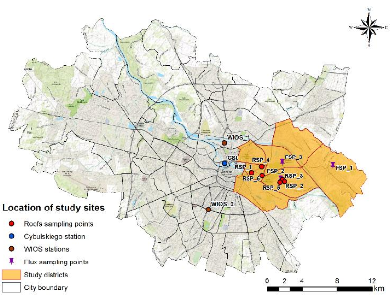
In the case of the limited observation network, the spatial interpolation analysis was covered at the district level in the east part of the city of Wroclaw (Figure 2). The experimental plot in Wroclaw is particularly well suited for this project because it contains a complex mixture of anthropogenic and biogenic sources. The selected sites of the city of Wroclaw were chosen to represent the different degrees of anthropogenic influence on ecosystems in a city. The observations at these urban sites were combined with analysis of meteorological records, studies of local conditions, historical patterns of pollution rates and impacts of land-use changes. The aforementioned variables (meteorological data and topographic trends) were used in the optimization of interpolation results by considering anisotropy and interpolation parameters (e.g., neighbourhood type and number of sectors angle type, effective terrain weights, as specified in the ArcGIS Geostatistical Wizard extension), as well as in the analysis of the reflection of smooth/sharp changes on the interpolated maps.
Anisotropic semivariograms applied during the interpolation validation procedures were used to detected directional trends of seasonal CO2 concentrations by dominant wind routes. Moreover, the aforementioned procedures were undertaken to ensure that the high CO2 concentration events (interpolated surfaces with and without anisotropy) are dependent on the wind as a key meteorological factor that impacts the distribution of air pollutants is and also related to the weather events, e.g., anticyclonic circulations (lower wind speeds and calm conditions). Additionally, a variable search radius during cross-validation was determined based on a topography effect to cover the areas of emission spots (significant sources of GHGs and major roads).
Several analyses have been performed in the investigation of CO2 emissions in the urban environment. The urban CO2 fluxes were estimated using a combination of different measurement approaches: the first one concerned the flask sampling (in gas sampling bags) of atmospheric CO2 mixing ratios, significantly influenced by fossil fuel component; the second one involved collecting samples for analysis of ambient CO2 concentration depending on the contribution of biospheric components (soil-surface CO2 fluxes and dynamics of photosynthesis) under various land use/land cover categories; the third one included continuous measurement of diurnal variations in CO2 concentrations.
The measurements of atmospheric CO2 were considered at three specifications: sampling points on the roofs; experimental sites that show natural emissions of CO2 within an urban location (in the vicinity of the soil respiration sampling plots); and measurements at the nearby automatic measurement stations of air pollutants for the Polish Chief Inspectorate of Environmental Protection. Following that, samples of ambient air were collected from the rooftop of the buildings at various altitudes (height of 15–30 m) at 6 experimental sites. Three plots were established over the area encompassing different biome types—the most typical urban ecosystems: grasslands, forests, arable fields. This study used datasets derived and measured at the nearby two automatic measurement stations of air pollutants for the Chief Inspectorate of Environmental Protection (in Polish, GIOŚ), showing variations in CO:CO2 ratios. Moreover, diurnal measurements of atmospheric CO2 concentration were performed from the laboratory building “Cybulskiego station” located in the city center and surrounded by a dense network of roads and close to the Oder River channel. The measurements at the “Cybulskiego station” were considered as independent check-point of urban CO2 concentrations in seasonal and diurnal cycles over a one-year period. The significant changes in concentration over short periods of time, often higher than the local background signals of CO2 in the heating season, were governed by local anthropogenic sources. Concentrations lower than the background CO2 time series usually reflect local sinks (biological CO2 fixation via plant photosynthesis) in the vegetation season.

2.3. Spatial Analysis and Modelling in the Geographical Information Systems (GIS)

The study investigates the relationships between field-determined seasonal CO2 concentration patterns and interpolated data at the specified sites across the study area, considering both related meteorological conditions and in-between the sampling points distance. The interpolated CO2 distribution is combined with a linear regression (LR) model of spatial and temporal trends of CO2 to estimate the impacts on a variance between time periods (for the vegetation and heating seasons) in response to terrain attributes and climatic variables of the area of interest. The approach is based on simple regressions that assume the relationship between observed mean CO2 concentration and effects of meteorological factors on both the temporal magnitude and spatial patterns of the carbon cycle. The resulting data (residuals of LR model) were then utilized to interpolate seasonal mean CO2 concentrations for the target locations and compared with original interpolator.
The observation size was examined by the distribution of CO2 on samples for the vegetation and heating periods. The Pearson correlation matrix was applied to estimate the relationships between the CO2 level and environmental variables (air temperature, relative humidity, atmospheric pressure, wind direction, and wind velocity) during the measurements. Multiple linear regression was also employed for each individual sampling site to examine the effect of meteorological factors on the seasonal cycle of CO2 in an urban area. The regression and correlation analysis performed using the least-squares method were conducted in the OriginPro 2019 software workspace.
The accuracy of observed and predicted CO2 distribution data within the study area is compared by applying GIS-based interpolation methods for point-sampled values by filling missing values in data sets of atmospheric CO2 monitoring. The interpolation analysis comprises hourly averages of atmospheric CO2 concentrations collected at the nine sites (roofs sampling points and flux sampling points) between July 2017 and August 2018; three sampling points (WIOS stations and Cybulskiego station) were used for verification purposes, as shown in Figure 2. The Tukey pairwise comparison between observations (t-tests: two-sample assuming) was used to evaluate the significance of differences in values of CO2 collected at each of the sampling points. A p-value (p = 0.05) was considered as statistically significant at measurement locations.
The analysis was carried out for the mean daily variation of CO2 levels in the study area. To capture the seasonal pattern of the CO2 concentration, the data attributed to each sampling location were further averaged. The averages for each measurement point were weighted in consideration of the site-specific data quality and completeness rate: missing observations were excluded from the dataset. The weighting factors used in the above calculation were geographic variables, such as topography, and land-uses of sampling sites (urban greenery represented by grasslands, forests, arable fields, e.g., “FSP_1-3” places) and emissions information, including the distance to the nearest major emission sources, and traffic intensity nearby (sites, located near heavy traffic roads, e.g., “RSP_1” and “RSP_6”), other observations with the pollutant of interest (e.g., “WIOS_1-2” measurement stations). Seasonal average CO2 concentrations taken at specific points were then interpolated. Predictions based on seasonal time scale were compared with monitoring data for the assessment of the spatial interpolation methodologies.
The different interpolation methods, such as inverse distance weighting (IDW), the natural neighbor approach, and interpolation based on a triangulated irregular network, Voronoi polygons were tested to analyze capabilities and select which method is best suited for fulfilling data gaps in CO2 measurements from selected nearby sampling locations. The various methods of interpolation work slightly differently, e.g., in a way to the shape of some mathematical function that is applied to the whole area of interest. IDW interpolation and spline are two deterministic methods that create surfaces from samples based on the extent of cell similarity or degree of smoothing [42]. However, a spline mathematical function crosses exactly through each sample point, while IDW crosses through none of the points [43]. In the IDW-based spatial interpolation method, the value at the unknown location (x, y), u(x, y) is calculated as the weighted average of the measurements at the monitoring sites, and the equation is (1) [9]:
u ( x , y ) =   n = 1 N u n ( x n ,   y n ) d n n = 1 N 1 d n  
where d n =   ( ( x x n ) 2 + ( y y n ) 2 ) i is a commonly squared distance (i = 2).
IDW is mostly used in pollution sampling and health science; kriging often used in soil science and geology, as well as in the field of atmospheric data analysis [12]. Spline interpolation is the best method to predict the smoothly varying surfaces of phenomena like temperature [44]. The interpolated value at the spline algorithm can be expressed as (2) [45,46]:
S ( x , y ) = T ( x , y ) + j = 1 N λ j R ( r j )
where j = 1, 2, …, N; N—the number of points; λj—coefficients found by the solution of a system of linear equations; rj—the distance from the point (x, y) to the jth point.
There are two spline methods: regularized and tension. A regularized method creates a more elastic, gradually changing surface, while a tension spline usually creates smoother surfaces of the same sample points [47]. The tension curve is flatter than the regularized curve and forcing the estimates to stay closer to the sample data. The tension spline uses only first (slope) and second derivatives (rate of change in slope), when regularized includes the first second, and third derivative (rate of change in the second derivative) in the Spline computing [47]. Spline with a tension function is given by (3) [48]:
ϕ ( r ) = ln ( σ · r 2 ) + K 0 ( σ · r ) 2 + C E  
where r—distance between the prediction point and the sample; σ—tension parameter; E1—exponential integral function; CE—constant of Eulero (0.577215); K0—modified Bessel function.
The triangulated irregular network (TIN) interpolation typically used for high-precision modelling of smaller areas, e.g., in engineering areas [49]. Natural neighbour interpolation is based on the Voronoi tessellation of irregular distributed points, a network/region generated around each location in the data set can be written as (4) [19,50]:
w i =   Area ( V ( q )   V ( S i ) ) Area ( V ( q ) )  
where si the natural neighbours of q and V(si) their associated regions in the original Voronoi diagram.
A geostatistical method, such as kriging, is one of the most complex interpolators and a powerful statistical technique based on sophisticated weighted average techniques for predicting values derived from the measure of relationship in samples [51]. The method considers both the distance and the degree of variation between sample points when estimating values of unknown samples. The distance and direction between all possible pairs of data points are calculated to provide data on the spatial autocorrelation of the sample point set on a particular surface [49]. The general mathematical formula for a kriging interpolation scheme using weights independent of the data is defined as (5) [52,53]:
Z · ( u ) =   a = 1 n λ ɑ ( u ) Z ( u ɑ )  
where Z(uα) is the random variable model at location uα; the uα’s are the n data locations, the λα(u)’s are the ordinary kriging weights for estimation of Z · (u).
Choosing the correct type of interpolation method depends on many factors e.g., the nature of the observed variable and the representation period; types of surface for modelling; and the features of the geographic area [54]. The characteristic of pollutants affects the determination of the interpolation method to use. The difference in variance between different data sets provides information with regard to the level of data smoothing in the interpolated surfaces. For instance, the Thiessen and IDW techniques stay in the range of the original observations, while kriging and spline can exceed the observed range and produce interpolated values both below and above the measured ones [55,56].
The quality of the sampling set also affects the choice of the interpolation method. The kriging interpolation is more sophisticated than other methods, however, the limited number of sampling points, non-regular datasets, and clustered location of points could affect the quality of the interpolated outputs [57]. In the case of poorly distributed or few sampling points within the study area, then the application of the IDW method is better [58]. The spline interpolation does not work well if observation points are close together and have extreme differences in values [47].
Prediction accuracy of different interpolation methods is often evaluated by a cross-validation technique. The idea of cross-validation is removing one data point and performing the interpolation using the data at the remaining locations [47,59]. Furthermore, a calculation of residuals between the measured value of the removed point and its estimation is executed. The procedure is repeated until each observation in turn out of the sample has been estimated from the remaining observations [60]. After completing cross-validation, some data points can be rejected, such as that contains large errors or requires refitting the trend and autocorrelation models.
The spatial autocorrelation between points must be quantified through the semivariogram model: circular, spherical, exponential, Gaussian, linear [61]. When the semivariance is plotted against the lag distance or separation distance between points, the plot is called semivariogram [59]. The semivariance function characterizes the spatial continuity between points and estimates spatial dependence between observations. These spatial structures of semivariogram help in identifying autocorrelation, replicating samples and finding the optimal parameters of interpolation control parameters [61]. The model error for each interpolation in cross-validation is evaluated by statistical means, such as the mean error (ME) and root mean square error (RMSE) [60]. RMSE indicates an interpolator that calculates the most reliable estimates at an unsampled location and shows a dominant pattern in the data series [62].

3. Results and Discussion

3.1. Summary of the Measured CO2 Concentrations

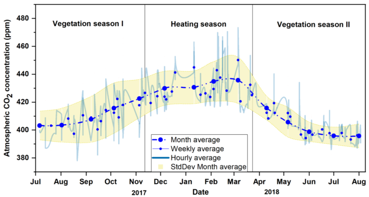
The analysis in this study is based on the average hourly time series of atmospheric CO2 concentrations measured at the surface level. The observation period was divided into the vegetative and non-vegetative phases according to the meteorological data. The vegetative stage (vegetation I: 6 July 2017–7 November 2017 and vegetation II: 29 March 2018–2 August 2018) was defined as the period when the daily mean air temperature increases above +5 °C, whereas the heating stage (8 November 2017–28 March 2018), refers to the phase of low temperatures (drops below +5 °C) when the need for home heating becomes quite high. The measured patterns of atmospheric CO2 concentrations followed a normal distribution for both periods (vegetation and heating), whereas over the whole study period (vegetation I, heating, vegetation II seasons) data were not significantly right-skewed from a normally distributed population (tested with the Shapiro–Wilk test). The overall distribution of observed annual CO2, however, provides statistically acceptable fits to the set of observations, the data kurtosis of a normal population curve was not reported as tested with the Shapiro–Wilk test (p < 0.05) in OriginPro 2019 software.
The time-series of measured CO2 levels indicated clear seasonality as a result of natural processes and human activity. In the vegetative season, the biological impact through the photosynthetic carbon fixation is dominant while the anthropogenic impact is minimized. Conversely, in the heating season, the anthropogenic CO2 sources are predominant, while photosynthesis uptake of CO2 by cover vegetation is negligible. According to the seasonal cycle of carbon dioxide, for most of the measurement sites, a marked increase in CO2 concentrations was observed in late autumn (from November) caused by a decrease in air temperature and related to higher energy consumption for electricity and heating purposes. The decline in concentration was recorded in early spring (at the end of March and April) due to the longer duration of sunshine and coupled changes in the vegetation distribution (plant respiration and uptake). The measured average concentrations for atmospheric CO2 ranged from 380 to 440 ppm with a mean of 412 ± 3.1 ppm for the vegetation season; and the maximum concentrations for CO2 were observed in the heating season, in the range of 410–470 ppm with a mean of about 430 ± 3.8 ppm in winter (Figure 3). Thus, the derived seasonal variation in atmospheric CO2 concentration reaches up to 25–30 ppm, which is consistent with the majority of previous studies [63,64,65,66].
The signals of measured CO2 for the study period also illustrate temporal variability in CO2 values over the sampling sites. Figure 4 shows the box plots of the median and interquartile range of CO2 concentrations at each sampling point. Analysis of variance (ANOVA) and a pairwise comparison Tukey test (p > 0.05) indicated a significant difference in the carbon dioxide rates observed for most of the study sites probably due to the distance between the sampling locations, and the influence of local sources (mainly transport activity and domestic heating sector). When analysing the differences separately for the vegetative and non-vegetative period, the seasonal pattern of CO2 concentrations was quite evident. At all measurement locations, atmospheric CO2 concentration was found to be higher in the heating period (from autumn to winter).
The compared means of atmospheric CO2 across the majority of the study sites were relatively close and do not demonstrate extreme values in the vegetation season (Figure 4). A peak in CO2 concentration (median mean of 414 ppm) was only measured at the “WIOS_2” on-road traffic station. Although slightly higher concentrations were measured in the “RSP_1” and “RSP_6” sites, located near heavy traffic roads. Three stations (“RSP_3”, “CSt”, “WIOS_1”) that were furthest from the heavily congested roads and associated with the urban greenery showed the lowest concentrations of CO2 (median mean below 397 ppm) observed during the vegetation season. From the results of pairwise comparisons of recorded CO2 in most of the observation locations, it can be concluded that there was a significant difference in CO2 measurements in the heating season. The winter CO2 maximum was also observed in the “WIOS_2” measurement station (median mean over 450 ppm). For some sites, such as “RSP_1” and “RSP_6” the measured atmospheric CO2 concentrations were characterized by peaks (median mean up to 440 ppm), predominantly caused by emissions from anthropogenic sources. Furthermore, the amplitude of the CO2 concentrations measured in the heating season indicated that the meteorological episodes (mainly, air temperature fluctuations) contributed significantly to the high variation in CO2 values within sampling groups (interquartile range on box plots).
The difference in the CO2 levels within and between the treatments (vegetative and non-vegetative period) can be explained by the contribution of different physical and physiological processes (respiration and photosynthesis components), complex emission source configuration and other multiple human-induced factors. The higher variability in meteorological conditions (duration of vegetation period, photosynthetically active radiation, precipitation, wind speed and direction) had a direct influence on the temporal patterns of atmospheric CO2 during vegetation and heating seasons. The results of the measurements of atmospheric CO2 were correlated with the meteorological conditions, represented in Table 1.
The Pearson correlation indicated moderately inverse correlation with air temperature (r = −0.43 and ρ = −0.41 for Pearson and Spearman statistics, respectively, p < 0.05) and a direct correlation with relative humidity (r = 0.28 and ρ = 0.22 for Pearson and Spearman statistics, respectively, p < 0.05). The CO2 concentrations were positively correlated with atmospheric pressure (r = 0.17 and ρ = 0.24 for Pearson and Spearman statistics, respectively, p < 0.05) and associated with a negative weak relationship with wind speed and direction (r = −0.22 and ρ = −0.19 for Pearson and Spearman statistics, respectively, p < 0.05). The observation size was examined by the multi-factor ANOVA, with the following model: y = −326.104 − 0.014 × x1 + 0.076 × x2 + 1.168 × x3 + 0.160 × x4 − 0.104 × x5 (where x1—air temperature, x2—air humidity; x3—atmospheric pressure; x4—wind velocity; x5—wind speed); and indicated that the air temperature parameter was the only key factor controlling the intensity of atmospheric CO2 for the vegetation and heating periods (F < 0.05, df = 711, p < 0.05). In general, the regression model results revealed that the local distribution of CO2 is dependent on the weather patterns, however, some meteorological influences were more specific and their effects were less obvious.

3.2. Geostatistical Analysis of Temporal and Spatial Variability of Atmospheric CO2 Concentrations

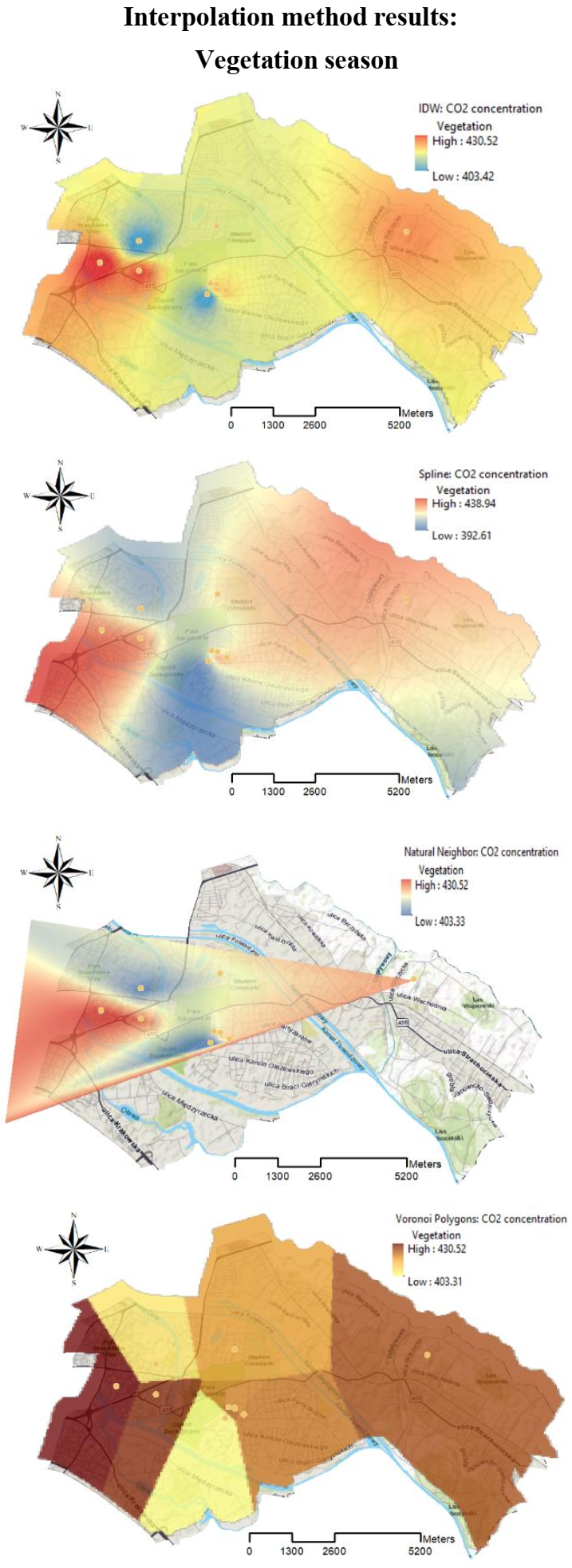
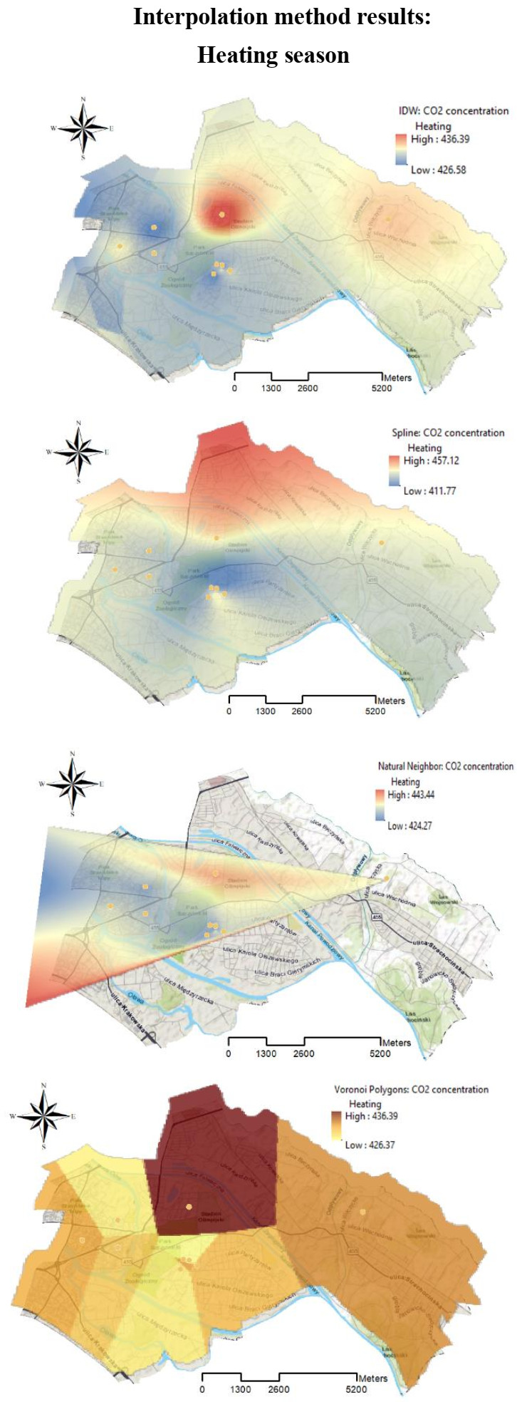
According to the results obtained from different interpolation methods, the quality of various predicted surfaces for the vegetation and heating seasons were identified. IDW, spline, and natural neighbour (NB) approaches showed some similarities in the produced surfaces. However, natural neighbour prediction led to accurate values mainly within a short distance in sample points location. IDW and spline interpolation gave a consistent, but poor performance for the seasonal CO2 distribution since the surface is highly susceptible to edge effects (unsampled locations) and clusterization (clustered sample points). The lowest and highest values obtained by Voronoi (Thiessen) polygons were representative of the original data range, however, the prediction had a much greater morphology of the map (high differentiation between colour ranges) and did not represent realistic dispersion conditions for CO2 emission.
In general, the IDW and spline methods can be accepted for the analysis of CO2 variability in Wroclaw over the vegetation and heating seasons compared to the natural neighbour interpolation and Voronoi (Thiessen) polygons. Prediction of seasonal changes in the atmospheric CO2 concentration using spline and IDW techniques had a relatively accurate level. Regarding the average prediction bias, the low ME values were obtained for the spline technique, which suggests low interpolation errors compared to the chosen interpolation methods. The predictive ability of the IDW method was generally lower compared to spline predictions (higher ME, RMSE values), probably due to a slight underestimation of the observed concentrations. However, it is also worth noting that IDW proves to be effective in identifying pollution hotspots from the interpolated surfaces; moreover, spline tends to have a ‘smoothening’ effect (see Figure 5 and Figure 6).
Every location (points) within a Thiessen polygon, due to the missing data at an unsampled area, had very little obvious trends within the dataset. The range of results obtained by IDW and spline interpolation was characterized by the minimum error variances (Table 2). However, the IDW approach strongly averaged data and did not produce values higher than the maximum and smaller than the minimum values of the observations. Overall, the differences of RMSE between IDW and spline were generally small, but IDW tended to higher errors, probably due to the uneven distribution of input points over the study area (edge effects and clusterization). The lower errors were introduced by natural neighbour estimating, as the interpolated values were close to the observed ones. However, the values predicted by natural neighbour were obtained only for the central part of the study extent, up to the contour of the data points. The absence of extrapolation results affected potentially large errors in the area outside sampling locations by the natural neighbour interpolation method.
The results showed that the choice of the correct type of interpolation method depends on many factors including the nature of the observed variable, size of the sample dataset used on spatial scale and the period on which it is represented. The interpolated surfaces (Figure 3 and Figure 4) of CO2 concentration differed significantly depending on the observation period (with the highest values in the heating season and lowest in the vegetation). The patterns of maximum concentration for vegetation and heating period changed direction angle mainly in the west and north parts of the prediction map. The CO2 values were more dispersed in the central part of the area, probably due to the lack of sampling points. Along with the central part and edges (northeast, southeast part) in the predicted CO2 concentration map, the unconvincing values were estimated.
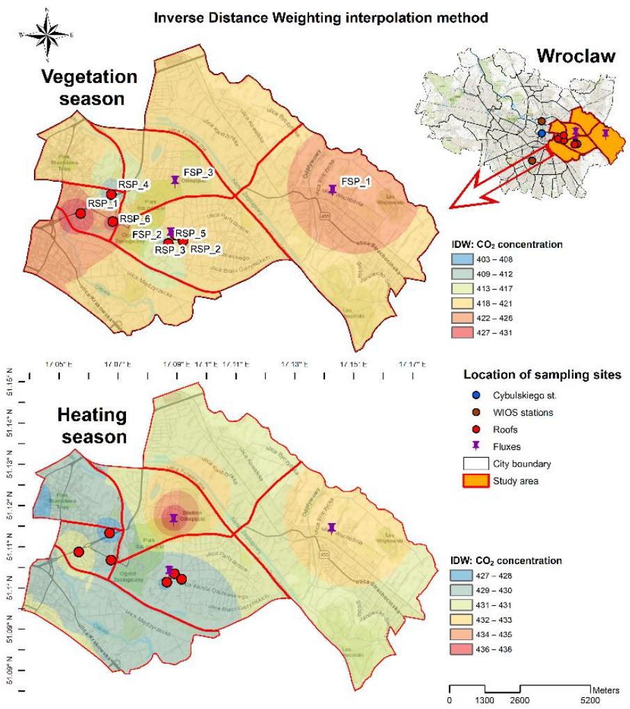
The IDW interpolated surface (Figure 7) represents the best quantitative and accurate results of CO2 dispersion in the atmosphere compared with other interpolators in this study. The predicted mean CO2 values were highest in the heating season (nearly 431 ppm) compared to the vegetation (mean 411 ppm). However, the IDW method works best for the dense enough, evenly-spaced sample point sets, that is why the formatted feature class cannot be sufficient to capture local CO2 concentration variations in the Wroclaw urban area.
We studied the anisotropy by managing search direction and showing its impact on the spatial correlation structure for a given, generally low number of observations (vegetation vs. heating season). The direction of anisotropy was determined by estimating semivariograms in multiplane directions. The semivariograms and semivariogram maps with search direction used to determine the presence and direction of anisotropy in the data in the vegetation and heating season (pattern of spatial correlation to be stronger in certain directions) are shown in Figure 8. Clear anisotropy that was found with direction labeled in semivariogram surface/maps, especially in the heating season, might suggest the spatial variability of the observed data. In general, the spatial correlation of the data in the direction perpendicular to that represented in Figure 8 is lower than that parallel to it, whereas the anisotropic model reaches the sill more rapidly.
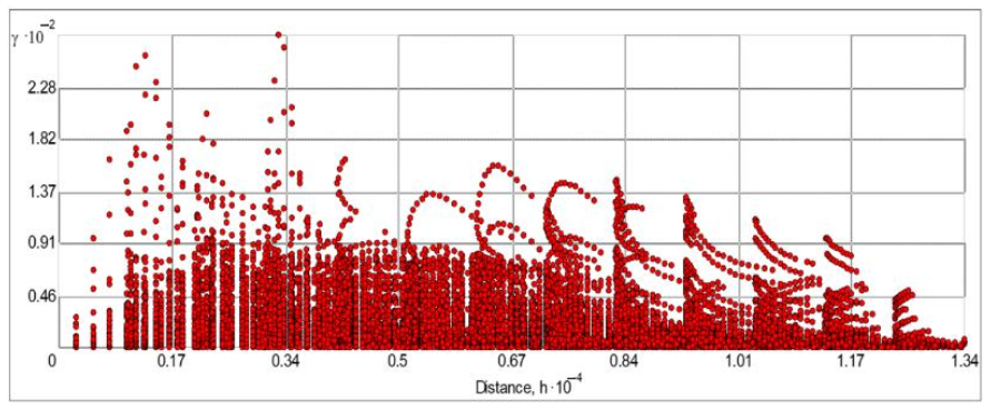
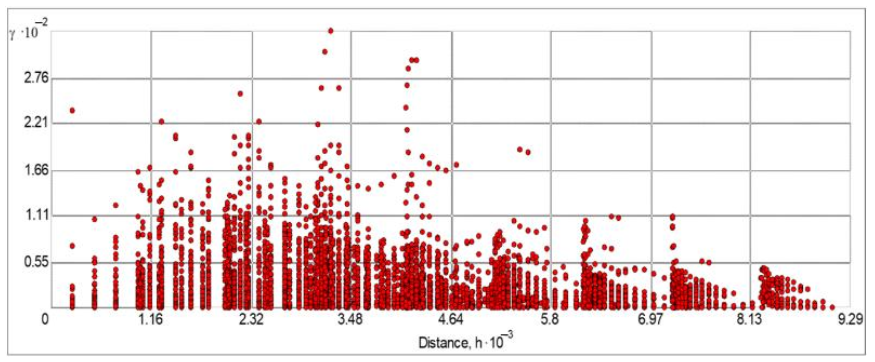
Normally, with the semivariogram, the variation of the values should increase with distance, but in this case, the clouds are not illustrating the expected results. The tendency of the geographic relationships is not within the expected range mainly due to the character of data collection. Some points are unevenly distributed, also located on the edges of the measured network or more influenced by neighboring points when they are more clustered. The semivariogram for the IDW method represents the high average rate of change of data property with distance and not significant consistency of the variable through space (Figure 9).
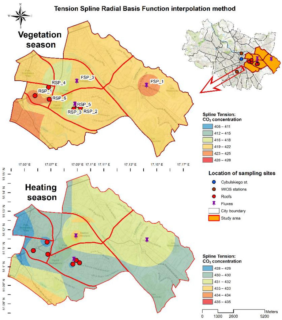
Based on the spatial similarity of the spline interpolated surface, it is difficult to highlight the obvious seasonal cycle of CO2 emissions from an urban area. The spline function modelled spatial distribution map shows no large differences in carbon dioxide concentration under the vegetation and heating conditions (Figure 10). The CO2 values are more dispersed, with higher values (419–420 ppm and 428–431 ppm for vegetation and heating period, respectively) in the central part of the area.
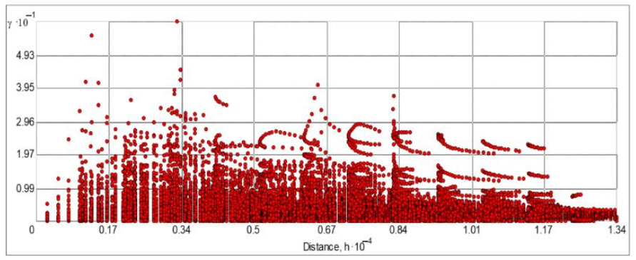
The level of model accuracy was tested also through semivariogram estimates of spatial dependence between observations for a particular spline-created surface. This information again raises the issue of the sampling distribution tendency, as well as reflecting non-uniform geometrical configuration and spatial resolution of the sampling points (Figure 11).
The Natural neighbour (NB) interpolation method was used as it generally works well with clustered scatter points [18]. A disadvantage of this technique is a limited interpolated surface up to data point contour; it does not extrapolate outside of the data locations. The natural neighbour method gives good results within uneven point distribution (Figure 12); it estimates the CO2 concentration in a similar pattern compared to the spline interpolation (an equal part of the produced surface). The general picture of the presented pollutant distribution on the right side and in the central part of the work extent is quite similar that obtained by the previous method. However, the absence of extrapolation results affects potentially large errors in the area outside sampling locations.
The spatial autocorrelation of the data points in the natural neighbour interpolated surface is visualized by the semivariogram in Figure 13. The semivariogram also represents the high average rate of change of the data property with distance and non-significant consistency of the variable through space.
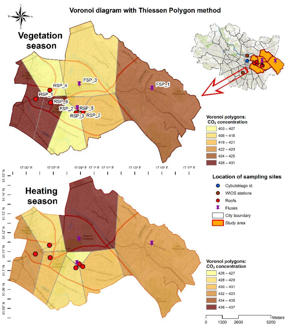
The Voronoi diagram with the Thiessen polygons was used to illustrate the stationarity of the dataset. Each Thiessen polygon contains only a single point input feature and represents the relationship for the data to their environment. Every location within a Thiessen polygon was closer to its associated point than to the input point of any other polygon. The trends shown in the Voronoi map (Figure 14) demonstrate the high variation with the dataset for the study area. The darker colors represent the higher rates of change of the CO2 concentration for the neighboring point dataset. The projected area due to the missing data at an unsampled location from the neighbouring observations had very little obvious trends within the dataset. This trend spreads in sites with no data—mostly north and south and northeast. Furthermore, this method showed the highest differences in observed and estimated CO2 values between vegetation and heating seasons.
The raster surface created with the spatial analyst tool in GIS software does not have semivariogram estimates of spatial dependence between observations for a particular Thiessen Polygons. The statistical model was estimated by calculating mean prediction error (MPE) and root-mean-square prediction errors (RMSE). The experimental results showed the main factors affecting the accuracy of interpolation are sampling density, sampling mode, and sampling location. The specific sampling datasets that do not reflect the complexity of the spatial characteristics rapidly increase errors of interpolation methods and the estimated values could be under-/overestimated. Organizing the sampling mode plays a key role in future predictions, for example, in regular-grid sampling (with cells of equal size), the spline interpolation method has the highest interpolation accuracy, and the IDW has the lowest interpolation accuracy.

3.3. Sampling Strategies for Optimization of the Effect of Interpolation

It is not easy to determine which interpolation is better by looking only at the spatial pattern of the interpolated surfaces. Multiple tools and approaches exist to answer the question about the differences among various methods. Several studies have demonstrated that the various spatial interpolation techniques perform differently depending on the type of inputs, the geometrical configuration of the samples, and spatial resolution [67,68,69]. In general, the performance of the kriging technique is better than the other studied interpolation methods, but it is more effective in predictions when the number of input points is higher in the monitoring network. The predictions of the kriging interpolation are greatly affected by the sampling configuration and spatial orientation of points of interest in the area under study.
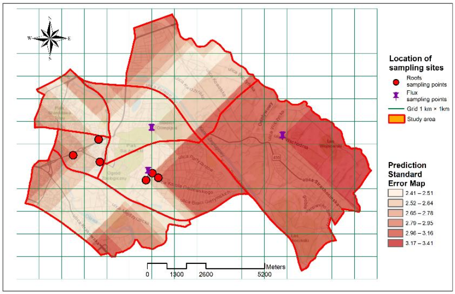
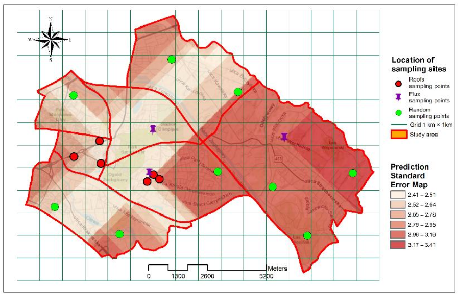
The best-interpolated outputs may only be when datasets used contain a sufficient number of sample points, evenly or high-density located in the study area. The limited number of observation points, as well as the isolated locations, both had a critical influence on the estimated CO2 distribution surface. The performance of chosen interpolators in the absence of spread datasets seems restricted for high-quality predictions. Unmeasured locations have the most impact on interpolated values and significantly entail the largest errors in the surrounding surface. As a result, it is critical that additional sampling points should be incorporated into further spatial estimates, especially in more problematic parts of the study area (edges and central). Regardless of the limitations of kriging interpolation on a number of data locations, the ordinary kriging prediction standard error map was developed in this study for a better representation of the spatial nature of atmospheric CO2 variations (Figure 15).
The design of the new monitoring locations was estimated using the following GIS interpolation methods: kriging technique (a prediction standard error map), create random points, and densify sampling network geoprocessing tools. To decide, which areas have the highest influence on the prediction surface, the prediction standard error (a kriging geostatistical layer) was computed. Furthermore, the spatially continuous prediction error map, associated with the kriging layer, was used as the selection criterion in determining the new sampling sites. The additional monitoring points in areas that are void of air quality measurements were distributed randomly by applying the random sampling approach with the optimization criteria (input weight raster). For this purpose, we prepared a probability raster taking into account additional layers such as land-use characteristics and large-size emission sources allocation and their combination through the use of the appropriate map algebra expressions. In this approach, the new sampling design depends not only on the monitoring network density but also on the importance of land uses, where the probability value is higher. Consistently, the prediction surface created by interpolation was improved by applying the most suitable error statistic layers to determine where the new monitoring sites should be built.
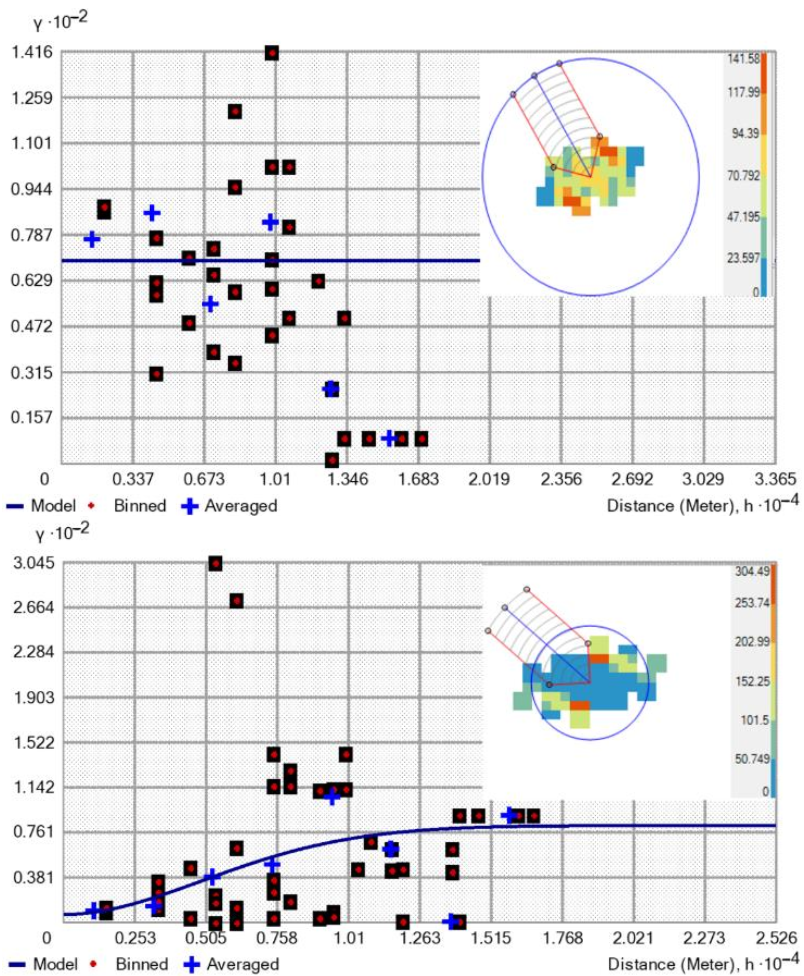
The next step for spatial analysis of these parameters was to form the empirical semivariogram that provides information on the spatial autocorrelation of datasets. The experimental semivariogram of a dataset for the vegetation and heating periods with its semivariogram curves is shown in Figure 16. There can be observed deviations of the points on the semivariogram from the averaged values—some points are above and below of the model curve. These variations could be the result of direction (anisotropy) trends, labeled on semivariogram surface/maps (see maps in a corner), or some unmeasurable physical process of pollution dispersion.
Spatial optimization from the kriging model indicates that there is a need to locate additional sampling points, especially in southern and southeast directions (values of the highest standard errors of prediction). A random sampling strategy was used to determine the new distribution of sample points by the reconstruction of the air sampling network density, especially in unmeasured locations. By using kriging interpolation (Figure 17) and the random points tool in ArcGIS software the error map was created, where the future sampling campaigns can be planned and a more realistic representation of CO2 distribution across the most problematic parts of the study area should be achieved.
This strategy would avoid biases related to data variability in the study area as compared to sampling at regularly spaced intervals. However, a random sampling strategy is largely dependent on the number of points and may not represent the important features of the data in complex terrain (e.g., local conditions, land cover, scope and sources of emission, spatial emission processes, etc.) and requires additional field inspections.
With the change of the sampling mode from regular-grid sampling to combined sampling, significant improvements in interpolation predictions were accomplished. Due to the much better positioning of sample locations in feature space, the reduced interpolation-error variance of the residuals was achieved. In the right-hand corner of the kriging predicted surface, the sampling intensity was increased to ensure adequate coverage of the observation network. The new sample locations were created in the bottom right and top right sides of the work extent to more effectively examine this area and shorten sampling intervals. Finally, the results obtained from the map of the optimal sampling scheme will lead to a better understanding of the spatial distribution pattern of pollutants in the city of Wroclaw and defining zones with differentiated intensity.
The performance of the interpolation techniques can be further improved by having a sufficient observation network with reasonable precision and including parameters related to the variable environmental parameters (e.g., wind, weather patterns). The critical requirements to more accurately capture the temporal and spatial variability of pollutant concentrations are high-density observational data conducted for a long-term period on a regular basis (e.g., daily). Since our measurements of CO2 levels were based on irregular sampling at a few sampling locations, we propose to include in the future sampling strategy unmeasured locations by discovering different spatial conditions (land-use characteristics) regardless of the actual distance to the surroundings of the existing monitoring stations, covering main emission sources in the study area, and capturing dependencies (spatial correlation) between the dispersion of air pollutants and meteorological data.
The future sampling strategy is based on searching for the problem features in areas of high uncertainty. Spatial optimization and validation procedures answered the research question of this part of the study, i.e., how many sample units (points) should be located to decide which interpolation technique is the most suitable for representation spatial and temporal distribution of atmospheric CO2 in given geospatial features, local climate, and meteorological conditions. In general, finding the optimal design of the spatial air quality monitoring network is a significant issue. The advantage is that an optimal sampling strategy leads to fewer sampling points and more cost-effective monitoring. The fact of this matter is that the well-planned urban-scale CO2 in situ emission observations with a focus on emissions according to source and geographic patterns, also comparing the measured data with city emission inventories, are strongly recommended.

4. Conclusions

Spatial interpolation methods are widely used in various fields of science for monitoring, mapping and spatial analysis of air pollution distribution. Five interpolation techniques (inverse distance weighting (IDW), spline, natural neighbour (NB) interpolation, interpolation based on a triangulated irregular network (TIN), Voronoi polygons, ordinary kriging) were compared in the present study for their ability to accurately produce the interpolated surface of atmospheric CO2 concentrations. Each interpolation method was tested for effectiveness in determining the CO2 distribution in the city of Wroclaw in two different periods (vegetation vs. heating seasons) from July 2017 to August 2018. The results obtained demonstrate that the acceptable quantitative and accurate results are obtained by IDW and spline interpolation compared to natural neighbour interpolation and Voronoi (Thiessen) polygons. The interpolated surface of CO2 level differs by almost 30% depending on the observation period (highest in the heating season, nearly 431 ppm, and lowest in the vegetation with mean of 417 ppm).
Because of the limited observation network which partly covers the analysed districts in the present case, there is no confirmed optimal interpolation method, only the optimal choice under certain circumstances. According to cross-validation estimates, the spline tension interpolation is identified as the most suitable tool for spatial, as well as temporal modelling of pollution in the studied geographic area. The high distinction between observed and estimated (interpolated) values for all surfaces was observed as the predicted surface is highly exposed to the present edge effects (unsampled sites) and clusterization (congestion of the sample points). This suggests that the location used to account for variations in atmospheric CO2 plays a critical role. The findings demonstrate that the interpolators should be used when the set of points is dense enough to capture the full extent of local surface variation.
In this study, the new sampling strategy was based on searching for the problem features in areas of high uncertainty. The performance of interpolation techniques was improved by the reconstruction of the air sampling network density, especially in unmeasured locations. By using kriging interpolation, the error map was created to determine where more information is needed when future sampling can be planned if necessary. Furthermore, the optimal number and the new randomly selected locations of sampling points were determined. In this case, the kriging technique was used not only for interpolating values in the site but also to directly estimate the degree of uncertainty associated with a map prediction. As a result of optimization, the more realistic representation of CO2 distribution across the more problematic parts of the study area was achieved. This is due to the much better positioning of sample locations in feature space, which results in a reduction of the interpolation-error variance of the residuals.
In general, based on the GIS tools, the results of in situ measurements can be represented as the data interpretation and visualization of related time series of air CO2 concentrations. Then, the urban air pollution maps with used parameters can accurately identify the areas of high concentration of GHGs, which would likely enable cities to manage their efforts better and set realistic targets of emission reduction. This study, however, left several questions unanswered, in particular regarding the optimal interpolation technique for the specific geospatial features, distribution of local emission source types (anthropogenic and biogenic) and contributions of atmospheric transport to the observed seasonal cycles of CO2. The fact of the matter is that the optimization of the air quality monitoring network for carbon dioxide for a medium-large city is a significant issue and requires advanced interpolation and modelling methods to handle time series with large gaps in measurements.

Author Contributions

Conceptualization: Y.B., J.B.; methodology: Y.B., J.B., M.G., I.S.; software: Y.B., J.B.; validation: Y.B., J.B., M.G., I.S.; formal analysis: Y.B., J.B., M.G., I.S.; investigation: Y.B., M.G., I.S.; resources: I.S.; data curation: Y.B., I.S.; writing—original draft preparation: Y.B.; writing—review and editing: Y.B., J.B., M.G., I.S.; visualization: Y.B.; supervision: J.B., M.G., I.S.; project administration: I.S.; funding acquisition: I.S. All authors have read and agreed to the published version of the manuscript.

Funding

This paper was co-financed within the “Excellent Science” program of the Polish Ministry of Science and Higher Education.
Atmosphere 12 00384 i001

Institutional Review Board Statement

Not applicable.

Informed Consent Statement

Not applicable.

Data Availability Statement

Not applicable.

Acknowledgments

The authors acknowledge the Department of Experimental Petrology, Institute of Geological Sciences at the University of Wroclaw for providing access for the use of CRDS analyzer Picarro G2201-i on CO2 measurements.

Conflicts of Interest

The authors declare no conflict of interest.

References

  1. Brondizio, E.S.; Solecki, W.; Leemans, R. Climate Change: A Virtual Special Issue with Commentary for #COP21. By Eduardo S Brondizio, William Solecki and Rik Leemans. Available online: https://www.elsevier.com/connect/climate-change-a-virtual-special-issue-with-commentary-for-cop21 (accessed on 19 December 2019).
  2. Mbow, H.-O.P.; Reisinger, A.; Canadell, J.; O’Brien, P. Special Report on Climate Change, Desertification, Land Degradation, Sustainable Land Management, Food Security, and Greenhouse Gas Fluxes in Terrestrial Ecosystems; Smith, P., Howden, M., Krug, T., Masson-Delmotte, V., Mbow, C., Pörtner, H., Reisinger, A., Canadell, J., O’Brien, P., Eds.; FAO-IPCC: Rome, Italy, 2017. [Google Scholar]
  3. Ritchie, H.; Roser, M. CO2 and other Greenhouse Gas Emissions. Published online at OurWorldInData.org. Available online: https://ourworldindata.org/co2-and-other-greenhouse-gas-emissions (accessed on 19 December 2018).
  4. Bezyk, Y.; Dorodnikov, M.; Grzelka, A.; Nych, A. Characteristics of temporal variability of urban ecosystem-atmosphere CO2, CH4, and N2O fluxes. E3S Web Conf. 2018, 44, 00013. [Google Scholar] [CrossRef] [Green Version]
  5. Jasek-Kamińska, A.; Zimnoch, M.; Wachniew, P.; Różański, K. Urban CO2 Budget: Spatial and Seasonal Variability of CO2 Emissions in Krakow, Poland. Atmosphere 2020, 11, 629. [Google Scholar] [CrossRef]
  6. Lauvaux, T.; Miles, N.L.; Deng, A.; Richardson, S.J.; Cambaliza, M.O.; Davis, K.J.; Wu, K. High-resolution atmospheric inversion of urban CO2 emissions during the dormant season of the Indianapolis Flux Experiment (INFLUX). J. Geophys. Res. Atmos. 2016, 121, 5213–5236. [Google Scholar] [CrossRef] [Green Version]
  7. Sun, W.; Liu, Z.; Zhang, Y.; Xu, W.; Lv, X.; Liu, Y.; Lyu, H.; Li, X.; Xiao, J.; Ma, F. Study on Land-use Changes and Their Impacts on Air Pollution in Chengdu. Atmosphere 2020, 11, 42. [Google Scholar] [CrossRef] [Green Version]
  8. Górka, M.; Lewicka-Szczebak, D. One-year spatial and temporal monitoring of concentration and carbon isotopic composition of atmospheric CO2 in a Wrocław (SW Poland) city area. Appl. Geochem. 2013, 35, 7–13. [Google Scholar] [CrossRef]
  9. Xie, X.; Semanjski, I.; Gautama, S.; Tsiligianni, E.; Deligiannis, N.; Rajan, R.; Philips, W. A Review of Urban Air Pollution Monitoring and Exposure Assessment Methods. ISPRS Int. J. Geo-Inf. 2017, 6, 389. [Google Scholar] [CrossRef] [Green Version]
  10. EPA. U.S. Environmental Protection Agency. Developing Spatially Interpolated. Surfaces and Estimating Uncertainty. EPA-454/R-04-004. November 2004. Available online: https://nepis.epa.gov/Exe/ZyPDF.cgi/P1002QG4.PDF?Dockey=P1002QG4.PDF (accessed on 1 March 2021).
  11. Mandelmilch, M.; Ferenz, M.; Mandelmilch, N.; Potchter, O. Urban Spatial Patterns and Heat Exposure in the Mediterranean City of Tel Aviv. Atmosphere 2020, 11, 963. [Google Scholar] [CrossRef]
  12. Matejicek, L. Assessment of Energy Sources Using GIS; Springer International Publishing: Berlin, Germany, 2017; pp. 195–220. ISBN 978-3-319-52694-2. [Google Scholar]
  13. Ristanović, B.; Cimbaljević, M.; Miljković, Đ.; Ostojić, M.; Fekete, R. GIS Application for Determining Geographical Factors on Intensity of Erosion in Serbian River Basins. Case Study: The River Basin of Likodra. Atmosphere 2019, 10, 526. [Google Scholar] [CrossRef] [Green Version]
  14. Vizcaino, P.; Pistocchi, A. Use of a Simple GIS-Based Model in Mapping the Atmospheric Concentration of γ-HCH in Europe. Atmosphere 2014, 5, 720–736. [Google Scholar] [CrossRef] [Green Version]
  15. Li, J.; Heap, A.D. Spatial interpolation methods applied in the environmental sciences: A review. Environ. Model. Softw. 2014, 53, 173–189. [Google Scholar] [CrossRef]
  16. Matejicek, L. Spatial modelling of air pollution in urban areas with GIS: A case study on integrated database development. Adv. Geosci. 2005, 4, 63–68. [Google Scholar] [CrossRef] [Green Version]
  17. Stocks, C.E.; Wise, S. The Role of GIS in Environmental Modelling. Geogr. Environ. Model. 2010, 4, 219–235. [Google Scholar] [CrossRef]
  18. Van Der Knijff, J.M.; Younis, J.; De Roo, A.P.J. LISFLOOD: A GIS-based distributed model for river basin scale water balance and flood simulation. Int. J. Geogr. Inf. Sci. 2008, 24, 189–212. [Google Scholar] [CrossRef]
  19. Deligiorgi, D.; Philippopoulos, K. Spatial Interpolation Methodologies in Urban Air Pollution Modeling: Application for the Greater Area of Metropolitan Athens, Greece. In Advanced Air Pollution; Nejadkoorki, F., Ed.; IntechOpen: London, UK, 2011. [Google Scholar]
  20. Li, L.; Zhou, X.; Kalo, M.; Piltner, R. Spatiotemporal Interpolation Methods for the Application of Estimating Population Exposure to Fine Particulate Matter in the Contiguous U.S. and a Real-Time Web Application. Int. J. Environ. Res. Public Health 2016, 13, 749. [Google Scholar] [CrossRef] [Green Version]
  21. Dashtpagerdi, M.; Sadatinejad, S.J.; Zare Bidaki, R.; Khorsandi, E. Evaluation of Air Pollution Trend Using GIS and RS Applications in South West of Iran. J. Indian Soc. Remote Sens. 2014, 42, 179–186. [Google Scholar] [CrossRef]
  22. Kianisadr, M.; Ghaderpoori, M.; Jafari, A.; Kamarehie, B.; Karami, M. Zoning of air quality index (PM10 and PM2.5) by Arc-GIS for Khorramabad city, Iran. Data Brief 2018, 19, 1131–1141. [Google Scholar] [CrossRef]
  23. Nichol, J.E.; Wong, M.S.; Wang, J. A 3D aerosol and visibility information system for urban areas using remote sensing and GIS. Atmos. Environ. 2010, 44, 2501–2506. [Google Scholar] [CrossRef]
  24. Wong, D.W.; Yuan, L.; Perlin, S.A. Comparison of spatial interpolation methods for the estimation of air quality data. J. Expo. Sci. Environ. Epidemiol. 2004, 14, 404–415. [Google Scholar] [CrossRef] [Green Version]
  25. Smolenski, R.; Beaulieu, J.; Townsend-Small, A.; Nietch, C. Spatial and Temporal Variations in Greenhouse Gas Emissions from an Agricultural Reservoir. In Proceedings of the American Geophysical Union Fall Meeting, San Francisco, CA, USA, 3–7 December 2012. [Google Scholar]
  26. Song, S.J. A GIS Based Approach to Spatio-Temporal Analysis of Urban Air Quality in Chengdu Plain. Int. Achieves Photogramm. Remote Sens. Spat. Inf. Sci. 2008, 37, B7. [Google Scholar]
  27. Zhao, Y.; Wu, B.F.; Zeng, Y. Spatial and temporal patterns of greenhouse gas emissions from Three Gorges Reservoir of China. Biogeosciences 2013, 10, 1219–1230. [Google Scholar] [CrossRef] [Green Version]
  28. Hutyra, L.R.; Duren, R.; Gurney, K.R.; Grimm, N.; Kort, E.A.; Larson, E.; Shrestha, G. Urbanization and the carbon cycle: Current capabilities and research outlook from the natural sciences perspective. Earth Future 2014, 2, 2014EF000255. [Google Scholar] [CrossRef] [Green Version]
  29. Levin, K.; Cashore, B.; Bernstein, S.; Auld, G. Playing it forward: Path dependency, progressive incrementalism, and the “super wicked” problem of global climate change. IOP Conf. Ser. Earth Environ. Sci. 2009, 6, 502002. [Google Scholar] [CrossRef]
  30. Pataki, D.E.; Alig, R.J.; Fung, A.S.; Golubiewski, N.E.; Kennedy, C.A.; McPherson, E.G.; Nowak, D.J.; Pouyat, R.V.; Romero Lankao, P. Urban ecosystems and the North American carbon cycle. Glob. Chang. Biol. 2006, 12, 2092–2102. [Google Scholar] [CrossRef]
  31. Fedra, K. Urban environmental management: Monitoring, GIS, and modelling. Comput. Environ. Urban Syst. 1999, 23, 443–457. [Google Scholar] [CrossRef]
  32. Luke, M.B.; Bräuer, I.; Gerdes, H.; Ghermandi, A.; Kuik, O.; Markandya, A.; Navrud, S.; Nunes, P.A.; Schaafsma, M.; Vos, H.; et al. Using Meta-Analysis and GIS for Value Transfer and Scaling Up: Valuing Climate Change Induced Losses of European Wetlands. Environ. Resour. Econ. 2012, 52, 395–413. [Google Scholar]
  33. Statistical Office in Wroclaw. Available online: https://wroclaw.stat.gov.pl/en/ (accessed on 17 December 2019).
  34. Kasprzak, M.; Traczyk, A. LiDAR and 2D Electrical Resistivity Tomography as a Supplement of Geomorphological Investigations in Urban Areas: A Case Study from the City of Wrocław (SW Poland). Pure Appl. Geophys. 2014, 171, 835–855. [Google Scholar] [CrossRef] [Green Version]
  35. Dąbek, P.B.; Jurasz, J. GIS estimated potential of rooftop PVs in urban areas—Case study Wrocław (Poland). E3S Web Conf. 2018, 45, 00014. [Google Scholar] [CrossRef] [Green Version]
  36. Sikora, S. Bioclimate of Wroclaw; Institute of Geography and Regional Development, University of Wroclaw: Wrocław, Poland, 2008; ISBN 978-83-9281193-2-5. [Google Scholar]
  37. Ogimet Weather Service. Available online: http://ogimet.com/cgi-bin/gsynres?ind=12424&lang=en&decoded=yes&ndays=2&ano=2018&mes=07&day=19&hora=12 (accessed on 17 December 2019).
  38. The Weather Online Ltd—Meteorological Services. Available online: https://www.weatheronline.co.uk/ (accessed on 30 November 2019).
  39. Górka, M.; Bartz, W.; Rybak, J. The mineralogical interpretation of particulate matter deposited on Agelenidae and Pholcidae spider webs in the city of Wrocław (SW Poland): A preliminary case study. J. Aerosol Sci. 2018, 123, 63–75. [Google Scholar] [CrossRef]
  40. Picarro G2201-i Analyzer User’s Guide Rev.; Picarro, Inc.: Sunnyvale, CA, USA, 2012; Available online: http://cires1.colorado.edu/jimenez-group/Manuals/PicarroG2401_Manual_rev_1_14_11.pdf (accessed on 9 March 2021).
  41. OpenStreetMap.org. Available online: https://github.com/openstreetmap/openstreetmapwebsite/tree/master/config/locales (accessed on 1 December 2019).
  42. Arseni, M.; Voiculescu, M.; Georgescu, L.P.; Iticescu, C.; Rosu, A. Testing Different Interpolation Methods Based on Single Beam Echosounder River Surveying. Case Study: Siret River. ISPRS Int. J. Geo-Inf. 2019, 8, 507. [Google Scholar] [CrossRef] [Green Version]
  43. Ikechukwu, M.; Ebinne, E.; Idorenyin, U.; Raphael, N. Accuracy Assessment and Comparative Analysis of IDW, Spline and Kriging in Spatial Interpolation of Landform (Topography): An Experimental Study. J. Geogr. Inf. Syst. 2017, 9, 354–371. [Google Scholar] [CrossRef] [Green Version]
  44. Childs, C. Interpolating Surfaces in ArcGIS Spatial Analyst. ESRI Education Services. 2004. Available online: https://www.esri.com/news/arcuser/0704/files/interpolating.pdf (accessed on 3 April 2019).
  45. Mitasova, H.; Mitas, L.; Harmon, R. Simultaneous Spline Approximation and Topographic Analysis for Lidar Elevation Data 6 in Open-Source GIS. IEEE Geosci. Remote Sens. Lett. 2005, 2, 375–379. [Google Scholar] [CrossRef] [Green Version]
  46. ArcGIS Pro. How Spline Works. Available online: https://pro.arcgis.com/en/pro-app/latest/tool-reference/3d-analyst/how-spline-works.htm#:~:text=The%20Spline%20tool%20uses%20an,exactly%20through%20the%20input%20points (accessed on 21 January 2020).
  47. Grundas, S.; Stepniewski, A. (Eds.) Advances in Agrophysical Research; IntechOpen: London, UK, 2013; p. 408. ISBN 978-953-51-1184-9. [Google Scholar]
  48. Garnero, G.; Godone, D. Comparisons between different interpolation techniques. Int. Arch. Photogramm. Remote Sens. Spat. Inf. Sci. 2013, XL-5/W3, 139–144. [Google Scholar] [CrossRef] [Green Version]
  49. ArcGIS Help. Available online: https://doc.arcgis.com/en/arcgis-online (accessed on 3 April 2019).
  50. Ledoux, H.; Gold, C. An Efficient Natural Neighbour Interpolation Algorithm for Geoscientific Modelling. In Developments in Spatial Data Handling; Springer: Berlin/Heidelberg, Germany, 2005; pp. 97–108. [Google Scholar]
  51. Kiš, I.M. Comparison of Ordinary and Universal Kriging interpolation techniques on a depth variable, case study of the Šandrovac Field. Min. Geol. Pet. Eng. Bull. 2016, 31, 41–58. [Google Scholar]
  52. Kumar, A.; Gupta, I.; Brandt, J.; Kumar, R.; Dikshit, A.; Patil, R.S. Air quality mapping using GIS and economic evaluation of health impact for Mumbai city, India. J. Air Waste Manag. Assoc. 2016. [Google Scholar] [CrossRef] [Green Version]
  53. Tyagi, A.; Singh, P. Applying kriging approach on pollution data using GIS software. Int. J. Electron. Electr. Eng. 2013, 4, 185–190. [Google Scholar]
  54. Wu, C.-Y.; Mossa, J.; Mao, L.; Almulla, M. Comparison of different spatial interpolation methods for historical hydrographic data of the lowermost Mississippi River. Ann. GIS 2019, 25, 133–151. [Google Scholar] [CrossRef]
  55. GIS Resources. A Knowledge Archive. Available online: http://www.gisresources.com/choosing-the-right-interpolation-method_2/ (accessed on 11 September 2019).
  56. Anselin, L.; Le Gallo, J. Interpolation of Air Quality Measures in Hedonic House Price Models: Spatial Aspects. Spat. Econ. Anal. 2006, 1, 31–52. [Google Scholar] [CrossRef]
  57. Meng, Y.; Cave, M.; Zhang, C. Comparison of methods for addressing the point-to-area data transformation to make data suitable for environmental, health and socio-economic studies. Sci. Total Environ. 2019, 06, 452. [Google Scholar] [CrossRef]
  58. Srivastava, P.K.; Pandey, P.C.; Petropoulos, G.P.; Kourgialas, N.N.; Pandey, V.; Singh, U. GIS and Remote Sensing Aided Information for Soil Moisture Estimation: A Comparative Study of Interpolation Techniques. Resources 2019, 8, 70. [Google Scholar] [CrossRef] [Green Version]
  59. Rodriguez, R. Integration of Topographic and Bathymetric Digital Elevation Model using ArcGIS Interpolation Methods: A Case Study of the Klamath River Estuary. Ph.D. Thesis, Geographic Information Science and Technology, University of Southern California, Los Angeles, CA, USA, 2015. [Google Scholar]
  60. Peckham, R.J.; Gyozo, J. Digital Terrain Modelling: Development and Applications in a Policy Support Environment; Springer: Berlin, Germany; New York, NY, USA, 2007. [Google Scholar]
  61. Karl, J.W.; Maurer, B.A. Spatial dependency of predictions from image segmentation: A variogram-based method to determine appropriate scales for producing land-management information. Ecol. Inform. 2010, 5, 194–202. [Google Scholar] [CrossRef]
  62. Luo, W.; Taylor, M.C.; Parker, S.R. A comparison of spatial interpolation methods to estimate continuous wind speed surfaces using irregularly distributed wind speed and direction data from the United Kingdom. Int. J. Climatol. 2008, 28, 947–959. [Google Scholar] [CrossRef]
  63. Jeleń, D. Anthropogenic Carbon Dioxide in Krakow City. Ph.D. Thesis, University of Science and Technology, Krakow, Poland, 2012. [Google Scholar]
  64. Pérez, I.A.; Sánchez, M.L.; García, M.Á.; Pardo, N.; Fernández-Duque, B. Statistical Analysis of the CO2 and CH4 Annual Cycle on the Northern Plateau of the Iberian Peninsula. Atmosphere 2020, 11, 769. [Google Scholar] [CrossRef]
  65. Butler, M.P.; Lauvaux, T.; Feng, S.; Liu, J.; Bowman, K.W.; Davis, K.J. Atmospheric Simulations of Total Column CO2 Mole Fractions from Global to Mesoscale within the Carbon Monitoring System Flux Inversion Framework. Atmosphere 2020, 11, 787. [Google Scholar] [CrossRef]
  66. Vardag, S.N.; Gerbig, C.; Janssens-Maenhout, G.; Levin, I. Estimation of continuous anthropogenic CO2: Model-based evaluation of CO2, CO, d13C(CO2) and d14C(CO2) tracer methods. Atmos. Chem. Phys. 2015, 15, 12705–12729. [Google Scholar] [CrossRef] [Green Version]
  67. Helfter, C.; Tremper, A.H.; Halios, C.H.; Kotthaus, S.; Bjorkegren, A.; Grimmond, C.S.B.; Nemitz, E. Spatial and temporal variability of urban fluxes of methane, carbon monoxide and carbon dioxide above London, UK. Atmos. Chem. Phys. 2016, 16, 10543–10557. [Google Scholar] [CrossRef] [Green Version]
  68. Super, I.; Stijn, N.C.D.; Visschedijk, A.J.H.; Denier van der Gon, H.A.C. Uncertainty analysis of a European high-resolution emission inventory of CO2 and CO to support inverse modelling and network design. Atmos. Chem. Phys. Discuss. 2019, 20, 1795–1816. [Google Scholar] [CrossRef] [Green Version]
  69. Rosenstock, T.S.; Sander, B.O.; Butterbach-Bahl, K.; Rufino, M.C.; Hickman, J.; Stirling, C.; Richards, M.; Wollenberg, E. Methods for Measuring Greenhouse Gas Balances and Evaluating Mitigation Options in Smallholder Agriculture. Introduction to the SAMPLES Approach; Springer International Publishing AG: Berlin/Heidelberg, Germany, 2016; pp. 1–13. [Google Scholar]
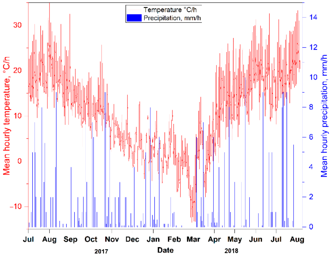
Figure 1. Monthly trends of the air temperature and precipitation observed at a meteorological station located at the Copernicus Airport Wroclaw from July 2017–August 2018.
Atmosphere 12 00384 g001
Figure 2. Location of study districts in the Wroclaw urban area. The measurement points are marked as: soil flux observation set/biogenic fluxes (violet pushpins), rooftop-level measurement sites (red points), location with on-site continuous diurnal series measurements (blue point); measurement stations operating by Inspectorate of Environmental Protection (dark red). The marks “RSP_1-6” indicate rooftop-level measurement sites, “FSP_1-3” soil flux sampling places, “CSt” means a location with continuous diurnal series measurements (“Cybulskiego station”), WIOS_1-2 are, respectively, measurement stations operating by Inspectorate of Environmental Protection. Base map source [41].
Atmosphere 12 00384 g002
Figure 3. Seasonal patterns of the measured mean atmospheric CO2 concentration in the sampling sites over the study period (vegetation I, heating, vegetation II, respectively) in July 2017–August 2018. A city-wide average for CO2 was computed by averaging daily values across all sites. Error areas indicate the standard deviation (2σ) of the means.
Atmosphere 12 00384 g003
Figure 4. Box plot of the measured atmospheric CO2 concentration in the sampling sites over the study period (vegetation vs. heating) in July 2017–August 2018. The box components indicate the median (horizontal line) and range between the 25th and 75th percentile of the measured values, respectively. The whiskers represent the highest and lowest 1.5 × IQR (interquartile range) of the mean data values. The various lower-case letters show which measurements for individual sampling points by comparing seasonal CO2 trends were significantly different. The marks “RSP_1-6” indicate rooftop-level measurement sites, “FSP_1-3” soil flux sampling places, “CSt” means a location with continuous diurnal series measurements (“Cybulskiego station”), WIOS_1-2 are respectively measurement stations operated by the Inspectorate of Environmental Protection.
Atmosphere 12 00384 g004
Figure 5. Interpolated surfaces of CO2 distribution in the Vegetation season. 3-D view in ArcScene obtained for selected interpolation techniques (top to bottom): Inverse Distance Weighting (IDW), Spline, Natural Neighbour (NB) interpolation, Voronoi (Thiessen) Polygons.
Atmosphere 12 00384 g005
Figure 6. Interpolated surfaces of CO2 distribution in the Heating season. 3-D view in ArcScene obtained for selected interpolation techniques (top to bottom): Inverse Distance Weighting (IDW), Spline, Natural Neighbour (NB) interpolation, Voronoi (Thiessen) Polygons.
Atmosphere 12 00384 g006
Figure 7. Geographic information system (GIS) coupling mapping of spatial CO2 distribution in the vegetation and heating seasons, a surface produced using the IDW interpolation method.
Atmosphere 12 00384 g007
Figure 8. The semivariogram cloud and anisotropic model based on the semivariogram maps of collected data in the vegetation season (top) and heating season (bottom).
Atmosphere 12 00384 g008aAtmosphere 12 00384 g008b
Figure 9. The semivariogram graph of the predicted points for average CO2 variation with distance, obtained from the IDW interpolated raster.
Atmosphere 12 00384 g009
Figure 10. GIS coupling mapping of spatial CO2 distribution in the vegetation and heating seasons, a surface produced using the tension spline radial basis function interpolation method.
Atmosphere 12 00384 g010
Figure 11. The semivariogram graph of the predicted points for average CO2 variation with distance, obtained from the spline tension interpolated raster.
Atmosphere 12 00384 g011
Figure 12. GIS coupling mapping of spatial CO2 distribution in the vegetation and heating seasons, a surface produced using the natural neighbor interpolation method.
Atmosphere 12 00384 g012
Figure 13. The semivariogram graph of the predicted points for average CO2 variation with distance, obtained from the natural neighbor interpolated raster.
Atmosphere 12 00384 g013
Figure 14. GIS coupling mapping of spatial CO2 distribution in the vegetation and heating seasons, a surface produced using the Voronoi diagram with the Thiessen polygons method.
Atmosphere 12 00384 g014
Figure 15. Ordinary kriging prediction standard error map with the grid (1 km × 1 km) within a particular study area.
Atmosphere 12 00384 g015
Figure 16. The empirical semivariograms with averaged values (fitted models by solid lines) and semivariogram maps of the ordinary kriging method from the dataset for the vegetation season (top) and heating season (bottom).
Atmosphere 12 00384 g016
Figure 17. A new sample locations pattern optimized with the ordinary kriging interpolation model within the study area.
Atmosphere 12 00384 g017
Table 1. Relationship between meteorological variables and observed CO2 concentrations at the study sites.
Environmental FactorsCorrelation CoefficientsAtmospheric CO2 Concentration
RSP_1RSP_2RSP_3RSP_4RSP_5RSP_6CStFSP_1FSP_2FSP_3WIOS_1WIOS_2Average of Sites
Vegetation season
Air temperature (°C)Pearson−0.19−0.30−0.51−0.47−0.57−0.52−0.62−0.21−0.11−0.16−0.31−0.49−0.43
Spearman−0.20−0.46−0.46−0.62−0.35−0.57−0.64−0.19−0.12−0.13−0.30−0.55−0.41
Atmospheric humidity (%)Pearson−0.08−0.070.310.210.560.320.120.28−0.28−0.170.170.360.28
Spearman−0.23−0.070.190.140.310.240.320.24−0.30−0.210.210.380.22
Atmospheric pressure (hPa)Pearson0.130.350.150.380.350.11−0.06−0.320.060.510.100.140.17
Spearman0.140.300.220.420.530.27−0.14−0.330.020.300.240.320.24
Wind velocity (m·s−1)Pearson0.110.230.11−0.22−0.48−0.160.510.270.320.24−0.21−0.23−0.22
Spearman0.120.210.09−0.15−0.37−0.110.330.210.390.11−0.18−0.18−0.19
Wind direction (deg)Pearson−0.21−0.13−0.31−0.12−0.25−0.160.060.05−0.19−0.45−0.29−0.11−0.19
Spearman−0.29−0.15−0.38−0.10−0.42−0.120.030.09−0.25−0.39−0.36−0.14−0.23
Heating season
Air temperature (°C)Pearson−0.13−0.16−0.31−0.19−0.18−0.41−0.21−0.31−0.36−0.19−0.26−0.35−0.37
Spearman−0.15−0.12−0.32−0.32−0.19−0.40−0.17−0.50−0.34−0.24−0.35−0.32−0.39
Atmospheric humidity (%)Pearson0.190.190.300.510.390.290.130.110.090.090.130.390.29
Spearman0.360.170.310.410.430.320.140.120.160.110.190.410.31
Atmospheric pressure (hPa)Pearson0.140.190.110.390.260.190.090.090.260.080.150.340.19
Spearman0.270.150.120.290.130.180.100.110.260.160.180.330.17
Wind velocity (m·s−1)Pearson−0.17−0.16−0.13−0.17−0.18−0.19−0.33−0.28−0.16−0.17−0.11−0.27−0.16
Spearman−0.19−0.13−0.11−0.18−0.21−0.23−0.34−0.27−0.25−0.19−0.18−0.16−0.14
Wind direction (deg)Pearson−0.15−0.11−0.18−0.14−0.17−0.26−0.35−0.48−0.39−0.15−0.26−0.17−0.17
Spearman−0.17−0.14−0.14−0.15−0.16−0.28−0.36−0.44−0.29−0.17−0.29−0.20−0.18
Table 2. Summary statistics of the selected interpolation methods: vegetation vs. heating season.
CO2 Concentration (ppm), Vegetation Season
Interpolation MethodsMinMaxMeanStd. dev.MERMSE
Observed Values384.31430.62407.418.35--
IDW403.42430.52416.972.39−0.138.74
Spline392.61438.94415.771.66−0.418.27
Natural Neighbor403.51420.51412.017.440.134.22
Voronoi Polygons403.31430.52418.411.61−0.659.17
CO2 Concentration (ppm), Heating Season
Interpolation MethodsMinMaxMeanStd. dev.MERMSE
Observed Values411.35455.93433.646.05--
IDW426.57436.39431.481.68−1.747.05
Spline411.76457.12434.441.37−0.856.88
Natural Neighbor424.27443.43433.854.640.833.81
Voronoi Polygons426.36436.39431.372.53−1.617.74
Publisher’s Note: MDPI stays neutral with regard to jurisdictional claims in published maps and institutional affiliations.