A Novel Convective Storm Location Prediction Model Based on Machine Learning Methods

Abstract

A weather radar is a frequently used device in remote sensing to identify meteorological phenomena using electromagnetic waves. It can observe atmospheric conditions in a wide area with a remarkably high spatiotemporal resolution, and its observation results are useful to meteorological research and services. Recent research on data analysis using radar data has concentrated on applying machine learning techniques to solve complicated problems, including quality control, quantitative precipitation estimation, and convective storm prediction. Convective storms, which consist of heavy rains and winds, are closely related to real-life and cause significant loss of life and property. This paper proposes a novel approach utilizing the given convective storms’ temporal properties based on machine learning models to predict future locations. The experimental results showed that the machine learning-based prediction models are capable of nowcasting future locations of convective storms with a slight difference.

1. Introduction

Convective storms are hazardous meteorological events that are accompanied by heavy precipitation, lightning, and strong winds. They influence various fields ranging from stopping human activities to losses of life and property. Consequently, it has been considered one of the primary goals in meteorological fields to make a short-term forecasting (or nowcasting) model. Despite the various approaches that have been introduced and widely used in practice over the years, nowcasting convective storms remains a challenging problem due to the complexity of the atmospheric conditions and relevant dynamical processes [1]. Although many devices and methods, including satellite, Doppler radar, and numerical weather prediction (NWP), are available to obtain useful meteorological information, the Doppler radar is the most preferred selection because it provides three-dimensional structures of the convective storms with a high spatiotemporal resolution by using rapid volumetric scanning with broad coverage [2]. These exceptional properties of the Doppler radar allow monitoring and analyzing properties of convective storms. Traditional radar-based nowcasting approaches consist of two broad categories: cross-correlation and centroid-based methods.

The cross-correlation based nowcasting method uses two-dimensional radar reflectivity data. It partitions the data into features and identifies the vector field that maximizes the correlation between identified features along consecutive time. A representative example of this type of method is TREC (Tracking Radar Echo by Correlation) [3,4]. The advantage of this method is that it can derive more precise speed and direction information. On the other hand, it is incapable of identifying and tracking individual convective storms, which cannot extract each convective storm’s quantitative characteristics. The centroid-based nowcasting method analyzes a series of radar reflectivity data obtained along time to identify convective storms and find their past trajectories. After that, it extrapolates the identified convective storms’ motion using a linear trend model to predict where they will be in the future. The advantages of this method are that it tracks individual convective storms effectively and provide their temporal properties. Indicative examples of this method are TITAN (Thunderstorm identification, tracking, analysis, and nowcasting) [5], SCIT (Storm Cell Identification and Tracking) [6], and TRACE3D [7].

Among those methods, TITAN has significantly influenced its post-researches by providing the following assumptions to predict future locations of convective storms: A storm tends to move along a straight line; A storm growth or decay follows a linear trend; Unexpected departures from the above behavior occur. Although those assumptions make the given problem straightforward, they make the forecasting model vulnerable to predicting the convective storms’ complicated movements. Recent research has been aware of these facts and suggested ways to improve the situation by applying machine learning, which can solve complex and nonlinear problems [8]. For example, Rossi et al. [9] uses the Kalman filter for probabilistic nowcasting to overcome the limited ability of deterministic approaches. Also, Han et al. [10] applies the support vector machine to predict one of the contiguous boxes containing a centroid of a convective storm in the future. Furthermore, Xingjian et al. [11] and Han et al. [12] utilize deep learning methods, which show superior performances in various practical fields, in a different context. Xingjian et al. [11] adopts a Convolutional LSTM to switch the nowcasting problem to a sequence-to-sequence problem, while Han et al. [12] utilizes a convolutional neural network to solve a problem caused by the manual construction of spatiotemporal features.

This paper proposes a novel approach using machine learning-based models to predict a convective storm’s future location. In other words, the proposed approach forecasts future centroid coordinates of the given convective storm using temporal properties from its trajectory. First, we derive distances and contained angles from vectors through centroid coordinates that lie nearby over time and have similar characteristics: they represent the given convective storms’ movement between sampling time. We selected several machine learning-based models as an autoregressive model [13] using the computed distances and contained angles. Furthermore, it is difficult to derive a sufficient number of time-varying characteristics when few convective storms in the given trajectory. Three distances and two contained angles can be derived, for instance, when the given convective storm has three observation results in the past. Therefore, this paper proposes additional novel method for dealing with insufficient time-varying characteristics (less than two observation results in the past) using machine learning-based models and other temporal features consisting of physical properties and descriptive statistics of the radar observation results between contiguous times. In summary, this paper provides four main contributions, as shown below.

• Machine learning-based approach to predicting future centroid coordinates of the given convective storm using temporal properties derived from its trajectory
• Flexible adjustments of sampling interval and maximum nowcasting range by increasing or decreasing the number of prediction models
• Applicable to analyze time-varying properties of the given convective storm along the same lines of the proposed method, including size-related parameters and variance of peak intensity
• Applicable to much meteorological analysis of which the future movement matters

This paper is organized as follows. Section 2 describes the data used in this paper. Section 3 introduces the methodology, and Section 4 analyzes and discuss the experimental results. Finally, the conclusions are presented in Section 5.

2. Data

The data used in this paper consists of 1872 three-dimensional composite radar data from 13 independent observation days from June to August 2018. The selected dates are concentrated in the summer because Korean summers are scorching and humid that are optimal conditions for forming convective storms. It is also necessary to obtain a more extensive observation range for precise analysis, mostly when the convective storms live long, although it is possible to examine trajectories of convective storms using observation data from a single radar. Therefore, as shown in Figure 1, this paper uses the composite radar data provided by Korea Meteorological Administration (KMA) combined with ten dual-polarization Doppler radars that observe the entire Korean region’s overall weather conditions. The size of composite radar data is 2049 × 2049 × 200, where the spatial resolution in x-axis, y-axis, and z-axis are 500 m, 500 m, and 50 m, respectively. Moreover, the observation interval is ten minutes.

From the three-dimensional composite radar data, 768 reference tracks consisting of 5384 convective cells, are manually extracted and verified by meteorological experts. As shown in Figure 2, many convective cells in the reference tracks survive for 70 min on average. The longest life in the observation is 340 min, and the shortest is 10 min. Considering that the machine learning model needs a sufficient amount of learning data, it is challenging to predict the given convective storm’s future locations further than a specific time due to a lack of observation cases with verification. Therefore, this paper limits prediction bounds up to 60 min at an interval of ten minutes.

Table 1. The number of learning data pairs for each model (Training:Test = 8:2).

Model	$(\mathit{t}+1)$	$(\mathit{t}+2)$	$(\mathit{t}+3)$	$(\mathit{t}+4)$	$(\mathit{t}+5)$	$(\mathit{t}+6)$
Number of data pairs	2004	1458	999	685	486	344
Training data pairs	1603	1166	799	548	389	275
Test data pairs	401	292	200	137	97	69

indicates the number of learning data pairs for each prediction model. From those data pairs, it is possible to extract various types of features, including descriptive statistics. Moreover, this paper divides training data and test data for each model because one of the essential issues for designing a machine learning model is to split training and test data. If not, the model delivers unreliable and over-optimistic prediction results due to the overfitting problem [14]. Table 1 shows that each data pair is divided into training and test data by applying an 8:2 ratio. For instance, 2004 data pairs for the $(t+1)$ prediction model are divided into 1603 and 401 data pairs for training and test.

3. Methods

In this section, the entire process for convective storm location prediction is elucidated. The operating principles of the proposed method follows the centroid-based method. Its process consists of three primary components as shown in Figure 3: identification, tracking, and location prediction.

Four kinds of observations obtained by dual-polarization radars are applied for the proposed convective storm prediction: corrected reflectivity (CZ), differential reflectivity (DR), cross-corrlation (RH), and vertically integrated liquid (VIL). CZ data is selected among the observations because the centroid-based prediction method [5] uses CZ data for the identification process. It groups contiguous points in the given radar data sequentially along the x-axis, y-axis, and z-axis. It is equivalent to hierarchical clustering with a single-linkage method using the three-dimensional kernel in a bottom-up fashion. The single-linkage clustering is adopted in this paper because it is better than the sequential approach in the time and computational complexities perspective.

It is crucial to match CZ’s coordinates to DR, RH, and VIL because there is a possibility not to one-to-one correspondence. In other words, the observed coordinate in CZ may not exist in DR, RH, or VIL due to observation properties. In the spatial feature extraction process, various properties are derived: two-dimensional and three-dimensional centroid coordinates, size-related features, and their descriptive statistics. Because CZ, DR, RH, and VIL have nonnegative values, entropies in image processing with base-2 logarithm are also computed as shown in Equation (1) by contemplating them as gray-scale images.

$$H\left(X\right)=\sum _{x}p\left(x\right){log}_2\left(\frac{1}{p\left(x\right)}\right)$$

(1)

where $p\left(x\right)$ indicates the normalized histogram counts of each identified convective storm in observation results.

Moreover, there are other newly proposed characteristics, named cluster VIL. The standard VIL in existing method is computed using Equation (2).

$$\mathrm{VIL}={\int }_{h_B}^{h_T}Md{h}^{\prime }=a{\int }_{h_B}^{h_T}{Z}^{b}d{h}^{\prime }=3.44\times {10}^{-6}{\int }_{h_B}^{h_T}{Z}^{\frac{4}{7}}d{h}^{\prime }$$

(2)

where $Z,h_B,h_T$ indicate CZ values, top and bottom altitudes, respectively. As shown in Equation (2), VIL integrates the reflectivity on the z-axis, which means that the altitude-based information will become indistinguishable. In other words, if several convective storms exist in the overlapping region on xy-plane with different altitudes, their distinctive characteristics can be squashed. Therefore, it is beneficial to utilize another VIL property of individual convective storm. As a result, two kinds of VIL-related features are generated in this paper. The identification method is straightforward: determine as a convective storm if a given object has a larger volume and higher reflectivity than thresholds $\{{\theta }_{\nu },{\theta }_Z\}=\{50{\mathrm{km}}^3,35\mathrm{dBZ}\}$ based on a sensitivity analysis presented by [5].

After the identification process, many valuable features can be extracted. Based on those features, it is possible to derive temporal features to understand the development of changes and trends of identified storms’ characteristics. As shown in

Table 2. The extracted temporal features from consecutive convective storms between (t) and $(t-1)$.

Number	Features	Descriptions
1	dist_3d	Euclidean distance (3D)
2	dist_w3d	Weighted Euclidean distance (3D)
3	dist_m3d	3D Euclidean distance (maximum reflectivity)
4	dist_ed	2D Euclidean distance (ellipse)
5	d_volume	Volume difference
6	d_area	Area difference (ellipse)
7	d_ecc	Eccentricity difference (ellipse with k=1)
8	d_mean_CZ	Mean CZ difference
9	d_max_CZ	Maximum CZ difference
10	d_min_CZ	Minimum CZ difference
11	d_median_CZ	Median CZ difference
12	d_iqr_CZ	IQR CZ difference (Inter-Quartile Range)
13	d_mode_CZ	Mode CZ difference
14	d_entropy_CZ	Entropy CZ difference
15	d_std_CZ	Standard deviation CZ difference
16	d_cv_CZ	CV CZ difference (Coefficient of Variation)
17	d_mean_DR	Mean DR difference
18	d_max_DR	Maximum DR difference
19	d_min_DR	Minimum DR difference
20	d_median_DR	Median DR difference
21	d_iqr_DR	IQR DR difference (Inter-Quartile Range)
22	d_mode_DR	Mode DR difference
23	d_entropy_DR	Entropy DR difference
24	d_std_DR	Standard deviation DR difference
25	d_cv_DR	CV DR difference (Coefficient of Variation)
26	d_mean_RH	Mean RH difference
27	d_max_RH	Maximum RH difference
28	d_min_RH	Minimum RH difference
29	d_median_RH	Median RH difference
30	d_iqr_RH	IQR RH difference (Inter-Quartile Range)
31	d_mode_RH	Mode RH difference
32	d_entropy_RH	Entropy RH difference
33	d_std_RH	Standard deviation RH difference
34	d_cv_RH	CV RH difference (Coefficient of Variation)
35	d_mean_VIL	Mean VIL difference
36	d_max_VIL	Maximum VIL difference
37	d_min_VIL	Minimum VIL difference
38	d_median_VIL	Median VIL difference
39	d_iqr_VIL	IQR VIL difference (Inter-Quartile Range)
40	d_mode_VIL	Mode VIL difference
41	d_entropy_VIL	Entropy VIL difference
42	d_std_VIL	Standard deviation VIL difference
43	d_cv_VIL	CV VIL difference (Coefficient of Variation)
44	d_mean_clus_VIL	Mean cluster VIL difference
45	d_max_clus_VIL	Maximum cluster VIL difference
46	d_min_clus_VIL	Minimum cluster VIL difference
47	d_median_clus_VIL	Median cluster VIL difference
48	d_iqr_clus_VIL	IQR cluster VIL difference (Inter-Quartile Range)
49	d_mode_clus_VIL	Mode cluster VIL difference
50	d_entropy_clus_VIL	Entropy cluster VIL difference
51	d_std_clus_VIL	Standard deviation cluster VIL difference
52	max_cv_VIL	CV cluster VIL difference (Coefficient of Variation)

, 52-dimensional temporal features are derived, such as Euclidean distances, trends of size-related and fundamental statistical features-related changes and trends. By including distance metrics, it is unnecessary to set a specific decision boundary by the users, unlike the traditional methods mostly refer to the TITAN method that uses a Hungarian algorithm. Instead of finding all possible links of given convective storms, this paper converts the problem as a binary classification. In other words, the tracking method in this paper finds a connection between a given identified convective storm at the time $\left(t\right)$ and identified convective storms at the time $(t-1)$ based on the extracted temporal features. When all connections between the identified storms at the time $\left(t\right)$ and $(t-1)$ are considered, the process is moved to the time $(t-1)$ and $(t-2)$. With the iterative manner, it is possible to track the convective storm in reverse order of time, as shown in Figure 3.

There are several successful prediction methods for the convective storm’s future location. Those methods are mostly based on the box-based method, which selects one of the adjacent boxes that will contain the future centroid coordinate of the given convective storm. This paper proposes a novel approach for convective storm location prediction from the time $(t+1)$ to $(t+6)$ by utilizing temporal properties in two-dimensional space. Finding the centroid coordinate of time $(t+1)$ at time $\left(t\right)$ needs to apply trigonometrical functions and $L_2$-norm. As shown in Figure 4, for instance, assuming that the goal is to find E coordinate using $A,B,C,$ and D, using Equations (3)–(6) can be derived coordinates for each axis.

$$x_E=x_D+{∥\overrightarrow{DE}∥}_2·cos\left({tan}^{-1}\left(\frac{y_D-y_C}{x_D-x_C}\right)-\theta (E,D,C)\right)$$

(3)

$$y_E=y_D+{∥\overrightarrow{DE}∥}_2·sin\left({tan}^{-1}\left(\frac{y_D-y_C}{x_D-x_C}\right)-\theta (E,D,C)\right)$$

(4)

$$\theta (E,D,C)=\widehat{\theta }(t+1)=f_{\mathrm{Angle}}\left(\theta (C,B,A),\theta (D,B,C)\right)$$

(5)

$${∥\overrightarrow{DE}∥}_2=\widehat{d}(t+1)=f_{\mathrm{Distance}}\left({∥\overrightarrow{CD}∥}_2,{∥\overrightarrow{BC}∥}_2,{∥\overrightarrow{AB}∥}_2\right)$$

(6)

where $\theta$ indicates the contained angle, ${∥·∥}_2$ implies $L_2$-norm, $f_{\mathrm{Angle}}(·)$, $\widehat{\theta }(t+1)$, $f_{\mathrm{Distance}}(·)$ and $\widehat{d}(t+1)$ mean the prediction models and their results of the contained angle and distance at time $(t+1)$, respectively. Repeatedly applying the same principle to time, it is possible to extend the model’s prediction range. In this paper, the maximum limit of prediction range is $(t+6)$, considering the given ground-truth dataset’s condition.

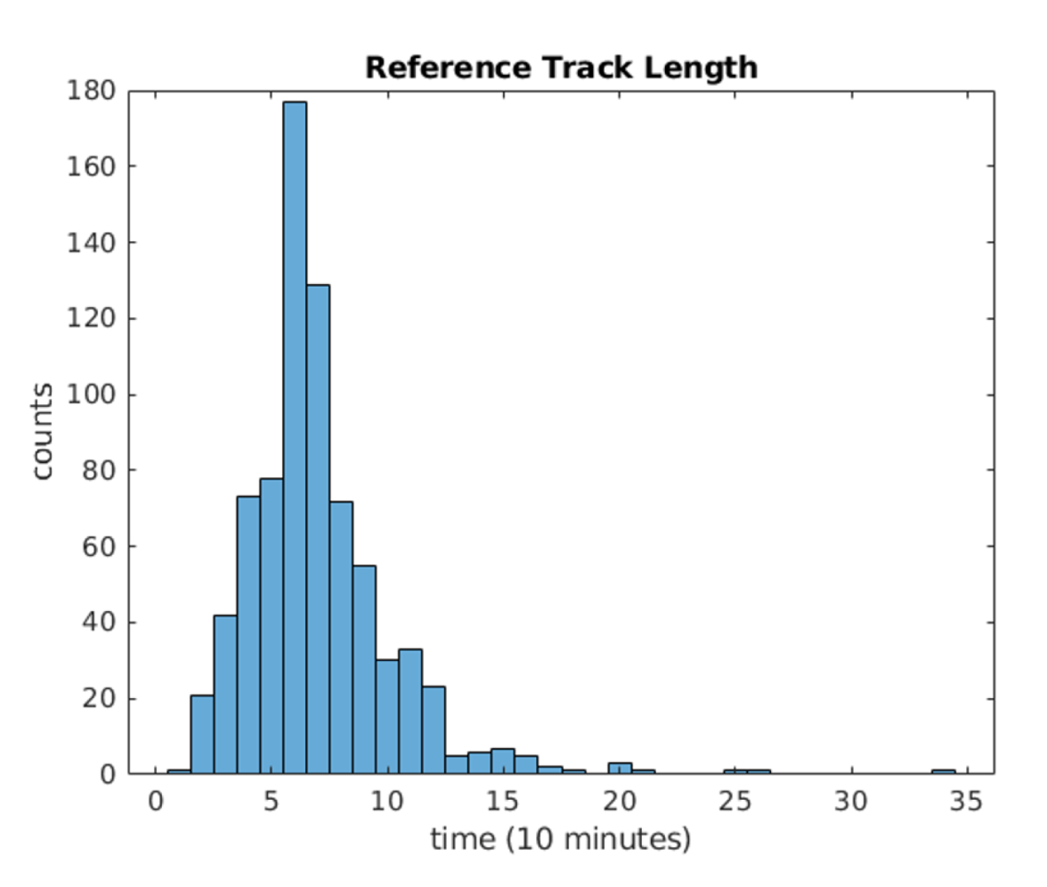
As shown in Equations (5) and (6), the three previous centroid coordinates can provide two contained angles and three $L2$-norms to angle and distance prediction models. It is a prerequisite of the proposed location prediction method: it must have a sufficient number of tracked centroid coordinates, more than three previous coordinates, for deriving temporal properties. However, at the beginning of the convective storm’s development, it is impossible to provide enough coordinates to derive temporal properties because its track has a short length.

This paper resolves the situation by dividing the trajectories into three occurrence cases, as shown in Figure 5: “Case 01” when the track has $\left(t\right)$ and $(t-1)$ coordinates, “Case 02” when the track has $\left(t\right)$, $(t-1)$, and $(t-2)$ coordinates, and “Case 03” when the track has $\left(t\right)$, $(t-1)$, $(t-2)$, $(t-3)$, and more coordinates. The track, which consists of only a coordinate at $\left(t\right)$, leaves out of consideration because it can be a noise signal and has insufficient properties to derive its movements through time. Considering that “Case 01” and “Case 02” have not enough previous centroid coordinates, they predict a distance between the current location and future location of given convective storms using 52-dimensional temporal features and machine learning-based models as shown in Table 2. Also, they adopt previous advancing angles by following the TITAN method’s first assumption: A storm tends to move along a straight line.

When the number of coordinates satisfies a specific condition regardless of observed and predicted, angles and distances are derived using nonlinear autoregressive models. In other words, the nonlinear autoregressive model forecasts the third future coordinate $({\widehat{x}}_{t+3},{\widehat{y}}_{t+3})$ in “Case 01”, the second future coordinate $({\widehat{x}}_{t+2},{\widehat{y}}_{t+2})$ in “Case 02”, and the first future coordinate $({\widehat{x}}_{t+1},{\widehat{y}}_{t+1})$ in “Case 03”, as shown in Figure 5.

4. Results and Discussion

This paper selected four representative machine learning methods: artificial neural networks (ANN) [15], linear regression model (LM) [16], random forests (RF) [17], and support vector regression (SVR) [18]. Those methods are well-known machine learning-based models and prove their capabilities to solve classification and regression problems in the real world. Moreover, this paper implemented the linear regression model with double exponential smoothing [19], which is the nowcasting method of TITAN, for comparison with maximum number of time points $n_t$ is 6 and weight parameter $\alpha$ is $0.5$. It can be a good criterion for evaluating the proposed machine learning-based methods because TITAN is a standard model for convective storm prediction. Considering that the proposed machine learning-based methods’ goal is to predict the future location of the convective storm, the nowcasting method of TITAN forecasts only the centroid coordinates by using Equation (7).

$$p_t=p_0+\left(\frac{dp}{dt}\right)\delta t$$

(7)

where $p_t$ and $p_0$ indicate the predicted and the current value, and $dp/dt$ is the estimated rate of change.

The nowcasting method of TITAN can also predict storm volume and the parameters of the projected-area ellipse. The predicted results are combined and evaluated like dealing with binary classification results. Namely, the prediction result is right when the forecasted storm position and actual radar echoes at the forecast time exist in a specific grid area. On the other hand, the prediction result indicates wrong when either the forecasted (failure case) or the actual echoes (false alarm case) at the forecast time does not exist in a specific grid area. It is not easy to apply the same evaluation process to the proposed methods because they predict only the centroid coordinates, making no way to derive failure and false alarm cases which allow deriving evaluation metrics such as the probability of detection (POD), critical success index (CSI), and false alarm ratio (FAR). Therefore, the root mean squared error (RMSE) is selected for performance verification in this paper, as shown in Equation (8).

$$\mathrm{RMSE}=\sqrt{\frac{1}{n}\sum _{i=1}^n{\left(\widehat{x_i}-x_i\right)}^2+{\left(\widehat{y_i}-y_i\right)}^2}$$

(8)

Table 3. Performance evaluations using root mean squared error (RMSE) for location prediction results.

			Case 01	Case 02	Case 03
Model	Hyper- Parameters	Predicted Time	Distance	Distance	Angle	Distance
ANN	1 hidden layer 10 neurons	$(t+1)$	0.6784	-	1.7012	0.3818
		$(t+2)$	-	0.1824	2.9922	0.7689
		$(t+3)$	-	-	1.9005	0.3814
		$(t+4)$	-	-	0.5228	3.9906
		$(t+5)$	-	-	1.4420	0.0269
		$(t+6)$	-	-	3.6229	1.7449
		Avg.	-	-	2.0303	1.2158
		Std.	-	-	1.1140	1.4822
LM	-	$(t+1)$	2.0859	-	6.0777	1.3242
		$(t+2)$	-	0.4730	2.6389	0.0714
		$(t+3)$	-	-	3.6844	0.6866
		$(t+4)$	-	-	0.8749	0.6694
		$(t+5)$	-	-	6.9876	0.2317
		$(t+6)$	-	-	10.4492	1.0764
		Avg.	-	-	5.1188	0.6766
		Std.	-	-	3.4364	0.4782
RF	25 subtrees 10 splits each	$(t+1)$	0.6121	-	4.8406	0.3120
		$(t+2)$	-	0.0913	0.1398	0.2722
		$(t+3)$	-	-	5.6896	0.3742
		$(t+4)$	-	-	0.5762	0.2214
		$(t+5)$	-	-	5.3583	0.5860
		$(t+6)$	-	-	9.1702	0.7567
		Avg.	-	-	4.2958	0.4204
		Std.	-	-	3.4128	0.2078
SVR	RBF kernel	$(t+1)$	2.5191	-	5.5931	0.3209
		$(t+2)$	-	0.1824	1.9501	0.1533
		$(t+3)$	-	-	3.7806	1.0203
		$(t+4)$	-	-	3.3121	1.1352
		$(t+5)$	-	-	5.3855	1.5833
		$(t+6)$	-	-	10.1840	2.0986
		Avg.	-	-	5.0342	1.0519
		Std.	-	-	2.8637	0.7386
TITAN	-	$(t+1)$	-	-	-	-
		$(t+2)$	-	-	-	-
		$(t+3)$	-	-	-	1.7137
		$(t+4)$	-	-	-	2.2190
		$(t+5)$	-	-	-	3.3513
		$(t+6)$	-	-	-	3.9340
		Avg.	-	-	-	2.8045
		Std.	-	-	-	1.0178

describes the performance of five models. As shown in Table 3, The hyperparameters of each machine learning-based model were empirically set to produce better results from the simple structure: ANN with a single hidden layer contained ten neurons with hyperbolic tangent sigmoid activation function, and an output layer contained a single neuron with linear activation function; RF with 25 subtrees with ten maximum splits; and SVR with radial basis function kernel. And the nowcasting method of TITAN has only four RMSE-based performances from $(t+3)$ to $(t+6)$ because it needs five historical data for predictions as mentioned above. On average, ANN shows better than others in the contained angle prediction, and RF is better than others in the distance prediction. Furthermore, almost all machine learning-based models proposed in this paper have better performance than the nowcasting method of TITAN. Considering that the angle and distance models are mutually independent, it is unnecessary to utilize homogeneous models for prediction. Therefore, this paper also conducts experiments using both ANN and RF for angle and distance prediction, respectively.

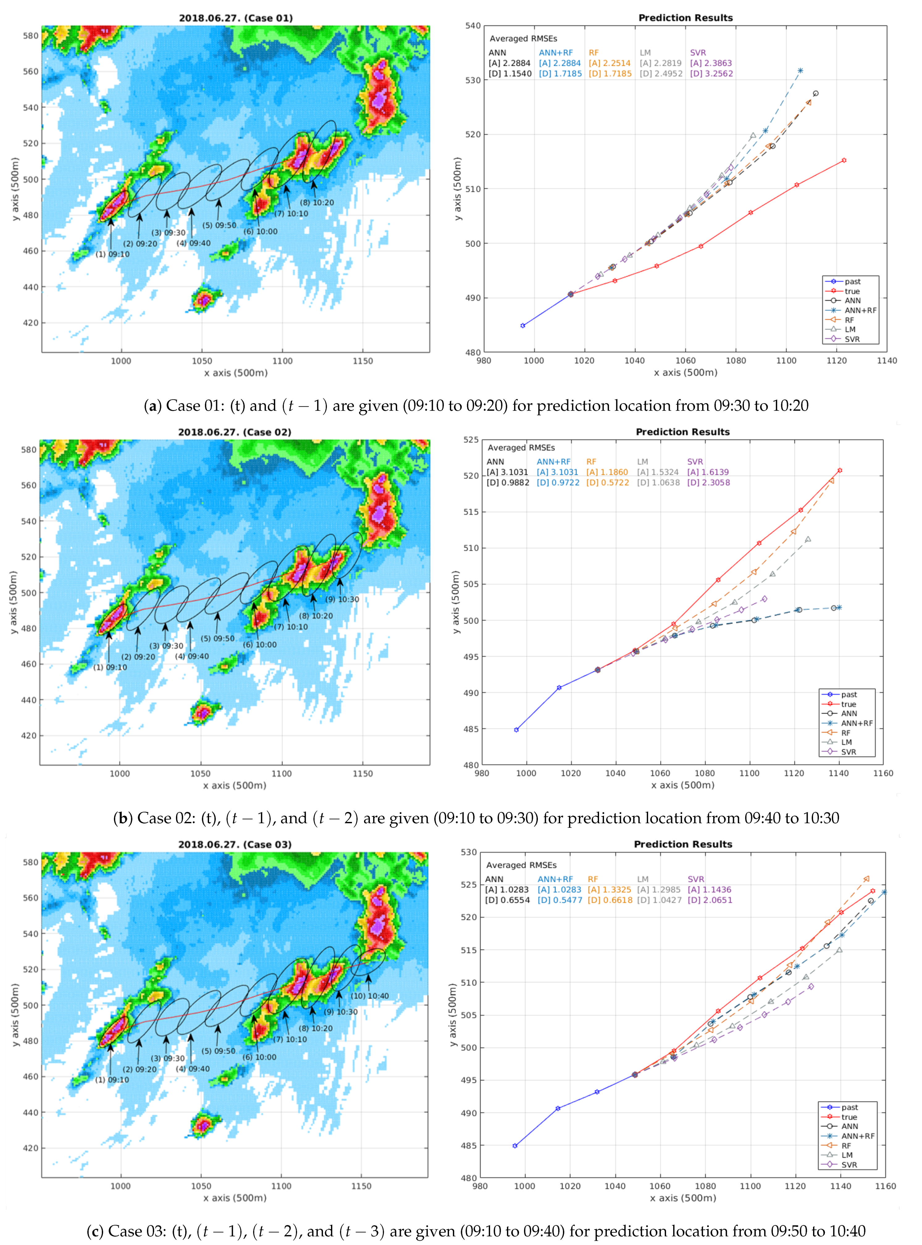
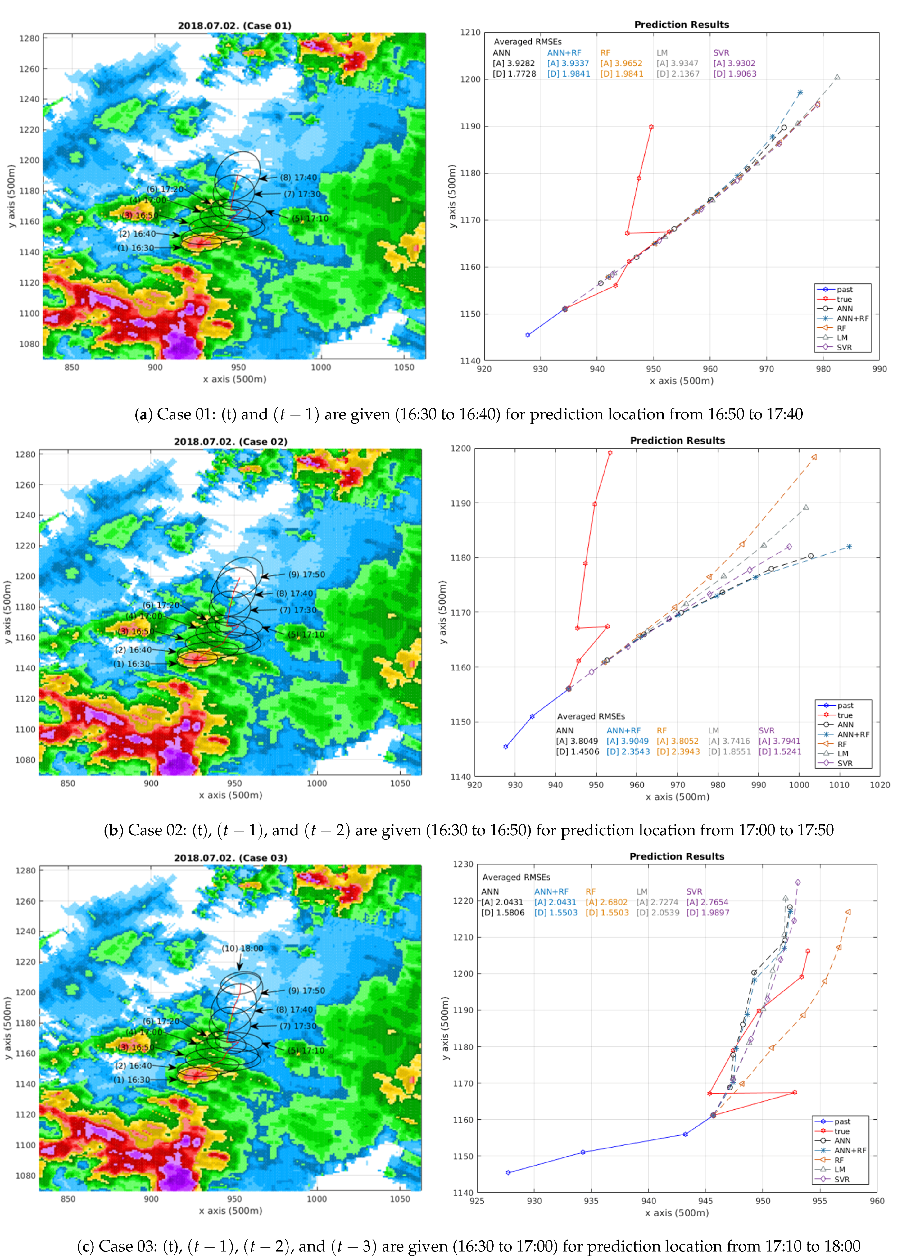
This paper selected two representative trajectory examples in the test data to visually compare and analyze the experimental results: the convective storm in the first example, as shown in Figure 6, moves linearly for 90 min along the coastline in the southern region of Korea; the convective storm in the second example, as shown in Figure 7, shows the sudden movement of the centroid coordinates along the inland area in the capital region of Korea. The different shapes of the trajectory and the different geographical characteristics can help analyze the accuracy and the efficiency of the proposed methods. Moreover, the experimental results, as shown in Figure 8, comparing the nowcasting method of TITAN as the standard model can demonstrate the proposed machine learning-based methods’ superiority.

Figure 6a illustrates the experimental results at “Case 01” when (t) and $(t-1)$ are given. As shown on the left side of Figure 6a, the objective is to derive future locations of (2), which are (3) to (8), using information derived from (1) and (2). Due to a lack of temporal movement information, all models draw deviated results from the reference track coordinates, as shown on the right side of the Figure 6a. Figure 6b indicates the experimental results at “Case 02” when (t), $(t-1)$, and $(t-2)$ are given. As shown on the left side of Figure 6b, the objective is to derive future locations of (3), which are (4) to (9), using information derived from (1) to (3). In this case, the RF-based method derives better results, as shown on the right side of Figure 6b, because the predicted locations exist near the reference track coordinates. The lowest RMSE values of the RF-based method provide numerical evidence for the results in Figure 6b. Other methods, which have greater RMSE values than the RF-based method, draw somewhat deviated (ANN, ANN+RF, and LM) or shrunk results (SVR). On the other hand, Figure 6c describes the successful experimental results at “Case 03” when (t), $(t-1)$, $(t-2)$, and $(t-3)$ are given. As shown on the left side of Figure 6c, the objective is to derive future locations of (4), which are (5) to (10), using information derived from (1) to (4). In this case, the combined method of ANN and RF derives better results, as shown on the right side of Figure 6c, because the predicted locations exist near the reference track coordinates. Although the RF-based method and ANN-based method seem to show similar performances, the trajectory’s detailed results prove the combined method slightly better than the RF-based or ANN-based method alone. Moreover, the RMSE values of the combined method substantiate the results, as shown in Figure 6c. Other methods draw somewhat deviated and shrunk trajectory results (LM and SVR). In summary, the RF-based method is useful when there are insufficient temporal properties, whereas the combined method of ANN and RF derives optimistic predictions when sufficient temporal data is guaranteed.

Likewise, Figure 7a describes the experimental results at “Case 01” when (t) and $(t-1)$ are given. As shown on the left side of Figure 7a, the objective is to derive future locations of (2), which are (3) to (8), using information derived from (1) and (2). Although all models draw nowcasting results close to the reference track coordinates from (3) to (5), they keep moving away from the reference after (6) due to insufficient temporal movement information, as shown on the right side of the Figure 7a. Figure 7b indicates the experimental results at “Case 02” when (t), $(t-1)$, and $(t-2)$ are given. As shown on the left side of Figure 7b, the objective is to derive future locations of (3), which are (4) to (9), using information derived from (1) to (3). In this case, all models draw more deviated results from the reference track coordinates, as shown on the right side of Figure 7b. On the other hand, Figure 7c represents the optimistic experimental results at “Case 03” when (t), $(t-1)$, $(t-2)$, and $(t-3)$ are given. As shown on the left side of Figure 7c, the objective is to derive future locations of (4), which are (5) to (10), using information derived from (1) to (4). In this case, the combined method of ANN and RF derives better results, as shown on the right side of Figure 7c, because the predicted locations exist near the reference track coordinates. The lowest RMSE values of the combined method of ANN and RF, as shown in Figure 7c, also verify the results. Other methods draw somewhat deviated results (ANN, RF, LM, and SVR). In summary, it is difficult to forecast when the centroid coordinates show sudden movements and there are insufficient temporal properties, whereas the combined method of ANN and RF derives promising results when sufficient temporal data is guaranteed.

Figure 8 illustrates the experimental results for comparison between the nowcasting method of TITAN and the proposed methods. As mentioned above, each model employs information derived from (1) to (6) because the hyperparameter ($n_t$) for the nowcasting method of TITAN is set to 6. Naturally, the common objective is to derive future location of (6), which are (7) to (10). As shown in Figure 8a, the nowcasting method of TITAN shows the worst result due to overpredict the distance, although it shows a similar linear movement. Furthermore, as shown in Figure 8b, the nowcasting method of TITAN not only deviates from the reference track coordinates but draws shrunk trajectory results due to the centroid’s abrupt direction change. Furthermore, the highest RMSE values of the nowcasting method of TITAN corroborate the results that the proposed machine learning-based prediction models are better, as shown in Figure 8a,b.

From the experimental results in Table 3, Figure 6, Figure 7 and Figure 8, the proposed machine learning-based method proves the following advantages than the nowcasting method of TITAN: First, it can relieve restrictions on the maximum number of time points. Second, it can learn how to deal with nonlinear and abrupt movements from data. Third, it can predict the given convective storms’ future locations more accurately under the same condition. Fourth, it can derive prediction results efficiently when the model has completed its learning process, whereas the nowcasting method of TITAN needs to compute the weighted linear regression every time.

5. Conclusions

Convective storms are hazardous meteorological events that are accompanied by torrential rain and strong winds. They influence various fields and have been considered primary goals in meteorological fields to make a nowcasting model. This paper proposes a novel method using machine learning-based models to predict a convective storm’s future location. In other words, the proposed approach forecasts future centroid coordinates of the given convective storm using temporal properties from its trajectory. The experimental results showed that the machine learning-based prediction models could forecast future locations of convective storms with superior performance to the nowcasting method of TITAN. As future work, we will consider exogenous variables as inputs, including satellite images, thermodynamic-related variables, numerical weather prediction results, wind, and buoyancy. The exogenous variables may derive promising results, such as improving prediction performance and dealing with more complicated trajectories.

Moreover, this paper proved that the machine learning-based model in a nonlinear autoregressive fashion utilizing only the dual-polarization radar data could derive the given convective storm’s future locations. However, there is a strong underlying assumption in the reference tracks: the connections between identified convective storms in contiguous time have a one-to-one correspondence. It is critical to deal with the mergers and splits of the convective storm in practical fields. Unfortunately, the splitting and merging cases of convective storms were insufficient, and most of them did not drastically influence the changes of the centroid coordinates’ positions. Considering that the machine learning-based methods cannot achieve expected performances if the learning data is insufficient and indistinguishable, we trained the proposed models under the mentioned assumption. As future work, we will apply classification methods based on machine learning for dealing with the splitting and merging cases of convective storms: classifier will determine the given convective storm will split, merge, or keep as it goes. We expect that the size-related input variables and their temporal trends significantly influence the classifier. With collecting a sufficient number of merging and splitting cases with meteorological experts’ verification, we expect that it is possible to derive promising results to handle the split-merge condition. Furthermore, it is possible to apply the proposed machine learning-based nonlinear autoregressive model to predict essential information, such as peak intensity of each convective cell and the trend of size changes through time.