Article

Maximum Instantaneous Wind Speed Forecasting and Performance Evaluation by Using Numerical Weather Prediction and On-Site Measurement

by
Atsushi Yamaguchi
and
Takeshi Ishihara
*
Department of Civil Engineering, School of Engineering, The University of Tokyo, Tokyo 113-8656, Japan
*
Author to whom correspondence should be addressed.
Atmosphere 2021, 12(3), 316; https://doi.org/10.3390/atmos12030316
Submission received: 3 January 2021 / Revised: 19 February 2021 / Accepted: 24 February 2021 / Published: 28 February 2021
(This article belongs to the Section Meteorology)

Abstract

:
A maximum instantaneous wind speed forecast methodology based on the autoregressive with exogenous inputs (ARX) model is proposed, in which numerical weather prediction and on-site measurement are used as inputs and the model parameters are estimated using non-parametric regression with forgetting factors. The accuracy of prediction using a proposed dynamic model is then evaluated and compared to the conventional static model output statistics (MOS) model. It is found that the prediction accuracy is improved by utilizing numerical weather prediction with a higher horizontal resolution. Finally, the predictability of the maximum instantaneous wind speed higher than 15m/s is evaluated using the receiver operating characteristic (ROC) curve and the area under the curve (AUC). The optimal quantile level of the maximum instantaneous wind speed is derived using a cost function.

1. Introduction

Many forms of infrastructure such as railways and roads are constructed in complex terrain in Japan. The operation and maintenance of these infrastructures are influenced by strong gusts of wind. For example, train operation has to be suspended when a certain value of instantaneous wind speed is recorded. This requires the forecasting of strong gusts of wind, including information on when the strong gust of wind happens and the intensity of the gust, with a forecast horizon of up to 24 h. Since decisions concerning operation are usually based on the instantaneous wind speed, forecasting of instantaneous wind speed is needed, as shown in Misu and Ishihara [1].
Kobayashi and Shimamura [2] proposed a method of predicting the instantaneous wind speed up to 15 min ahead based on the on-site measurement data and the Kalman filter for the application of train operation regulation. Hoppmann et al. [3] proposed a method for the prediction of instantaneous wind speed with a confidence interval up to two minutes based on past measurement data using a linear trend model for railway operations in Germany. Nevertheless, these methods based on previously measured data do not have the ability to perform forecasts up to 24 h ahead, and for this it is necessary to use forecast methods which can consider weather conditions, such as numerical weather prediction data.
Accordingly, much research has been conducted on wind power forecasting of up to 24 h, which is needed for power grid operation and power trading [4,5]. The most important part of wind power forecasting is the forecasting of the wind speed, which can be done using a combination of a physical model, such as numerical weather prediction (NWP) and a statistical model based on on-site measurement. Landberg [6,7] predicted the wind speed in a wind farm based on numerical weather prediction and measured wind speed using a statistical method called model output statistics (MOS). In MOS, the accuracy of the forecast is improved by using a linear regression model based on the available measurement data for each wind direction. Although this method reduces the bias of the forecast, long-term measurement data are required and the method cannot be used for cases in which the regression model changes depending on the season or in which the linear regression model is not applicable. Advances in wind power forecasting have been summarized by Sideratos and Hatziargyriou [8], Soman et al. [9], Giebel and Kariniotakis [10], Dittner and Vasel [11] and Dhiman et al. [12].
The autoregressive with exogenous inputs (ARX) model was proposed by Joensen et al. [13], in which the real-time measurement of the power generation output and numerical weather prediction are used as the input, and parametric regression with forgetting factors is used for the estimation of the model parameters and functions. They performed the forecast of the 1-h average wind power output up to 24 h ahead and verified the results at a wind farm in Denmark. The properties required for non-parametric probabilistic forecasts of wind power were pointed out by Pinson et al., along with an evaluation of their use [14]. Although the average power output can be forecasted with high accuracy by this model, no model has been proposed for the forecasting of the maximum instantaneous wind speed. Moreover, its applicability in complex terrain has not been clarified.
In this study, a forecast model for the maximum instantaneous wind speed using the ARX model is proposed in Section 2. Its applicability to maximum instantaneous wind speed forecasting in a mountainous area in Japan is then clarified and the effects of horizontal resolution on the numerical weather forecast data, used as inputs on the forecast accuracy, are investigated in Section 3. Furthermore, the predictability of strong gusts of wind with wind speeds higher than 15 m/s is quantitatively evaluated using receiver operating characteristic (ROC) curves and the area under the curve (AUC). The optimal quantile level of the maximum instantaneous wind speed is derived using a cost function.

2. Forecast Model

In this study, a model to forecast the maximum instantaneous wind speed up to 24 h ahead is developed based on the numerical weather prediction and on-site measurement of wind speed. Figure 1 shows an overview of the model. The first step of this model consists of a mean wind speed forecast model, a fluctuating wind speed forecast model and a peak factor forecast model. Each model performs a forecast based on numerical weather prediction and on-site measurement. Then, a maximum instantaneous wind speed forecast model calculates the expected valued of the maximum instantaneous wind speed by adding the fluctuating wind speed multiplied by the peak factor to the mean wind speed. Finally, the maximum instantaneous wind speed with a quantile level is evaluated by considering the forecast error of the expected value.
The numerical weather prediction and the on-site measurement, which are used as the input to the model, are first presented in Section 2.1. The mean wind speed forecast model, fluctuating wind speed forecast model, peak factor forecast model and the maximum instantaneous wind speed forecast model are then described in Section 2.2. Finally, non-parametric regression with forgetting factors is presented in Section 2.3.

2.1. Input Data

The Japan Meteorological Agency provides several numerical weather prediction datasets with different resolutions and forecast horizons, as shown in Table 1. In this study, the GPV-MSM dataset, which has the finest horizontal resolution of about 5 km at the surface, and the GPV-GSM dataset (Japan area), which has the second-finest horizontal resolution of about 20 km at the surface, are used in order to investigate the effect of the resolution of the NWP. The forecast interval of the GPV-MSM is three hours (i.e., eight forecasts per day), though only four forecasts per day are used for the sake of the comparison with GPV-GSM (Japan area). Among the forecast variables available in these NWPs, only the east–west component and the north–south components of the surface wind velocity are used as input data for the forecast model in this study.
In the proposed model, real-time on-site measurement of average wind speed, average wind direction, standard deviation of the wind speed and maximum instantaneous wind speed are used as input data. As described in Figure 1, the average wind speed and wind direction are the inputs to the average wind speed forecast model, the standard deviation of the wind speed is the input to the fluctuating wind speed forecast model, and the average wind speed and the standard deviation of the wind speed, as well as the maximum instantaneous wind speed, are the inputs to the peak factor forecast model. The averaging time of the wind speed can be set between 10 min and 1 h. In this study the averaging time is set to 30 min because the maximum instantaneous wind speed is forecasted every 30 min based on the 30-min average wind speed and the standard deviation of the wind speed for every 30 min. The forecast is also conducted every 30 min.
Figure 2 shows the forecast schedule when GPV-MSM is used as the input NWP. Forecast data is delivered online from the Meteorological Service Support Center approximately three hours after the initial time but may be delayed for up to three hours. For this reason, each forecast dataset is considered to become available six hours after the initial time and can be used for the wind speed forecast. For example, if the question of whether a strong wind event will occur during the daytime has to be determined at 6:00 am, the NWP data that can be used is based on the initial time at 21:00. This data is the forecast value from the initial value (21:00 the previous day) until 12:00 the next day, which is 39 h after the initial time.

2.2. Forecast Model

The NWP does not contain the effects of high-resolution terrain and surface roughness because of the limitation of the spatial resolution. In this study, the local forecast is used in which the local wind speed, affected by the high-resolution topography and surface roughness, is expressed as a function of wind speed and direction of NWP and is identified by non-parametric regression using the measurements and the NPW data. After k ^ steps ( k hours) at time t , the local wind speed forecast value | | u ¯ t + k | t local | is modeled as a function of the NWP wind speed | u ¯ t + k | t nwp | and NWP wind direction θ t + k | t nwp as shown in Equation (1), where the nearest neighbor of the output grid is used to extract exact-location wind forecasts from the NWP and is expressed as
| u ¯ t + k | t local | = f ( | u ¯ t + k | t nwp | , θ t + k | t nwp )
Note that k = k ^ Δ t . | u ¯ t + k | t nwp | and θ t + k | t nwp are the absolute value of the mean wind speed and wind direction of NWP, which can be calculated from the east–west component u t + k | t nwp and the northsouth component v t + k | t nwp of the wind speed, as shown in Equation (2).
| u t + k | t nwp | = ( v t + k | t nwp ) 2 + ( u t + k | t nwp ) 2 ,   θ t + k | t nwp = tan 1 ( v t + k | t nwp ,   u t + k | t nwp )
The function f ( | u ¯ t + k | t nwp | , θ t + k | t nwp ) is estimated using non-parametric regression with a forgetting factor, which is set to the value of 0.999, as proposed by Joensen et al. [13].
The local wind speed obtained using Equation (1) is considered to contain no bias component of error, but the phase error, which is originally included in NWP, is still included. To reduce this error for short-term forecasts, a model in which the weighted sum of the persistent forecast, which is a forecast that the future weather condition will be the same as the present condition, and the local forecast obtained by Equation (1) are used as the final forecast value, as
| u ¯ t + k | t pred | = a ( k , θ t + k | t nwp ) | u ¯ t meas | + b ( k , θ t + k | t nwp ) | u ¯ t + k | t local | ,
where a and b are the smooth functions of the forecast horizon k and the wind direction of NWP, and are estimated by non-parametric regression with the forgetting factor of 0.999 [13].
The fluctuating component of the wind speed σ t + k | t local is also assumed to be a function of the mean wind speed and wind direction of NWP.
σ t + k | t local = f σ ( | u t + k | t nwp | , θ t + k | t nwp )
Similar to the average wind speed, the forecast value of the fluctuating wind speed σ t + k | t pred is modeled as the weighted sum of the persistent forecast and the local forecast so that the phase error of the forecast can be reduced by Equation (5).
σ t + k | t pred = a σ ( k , θ t + k | t nwp ) σ t meas + b σ ( k , θ t + k | t nwp ) σ t + k | t local ,
where a σ and b σ are the smooth functions of the forecast horizon k and the wind direction of the NWP, and are estimated by non-parametric regression with the forgetting factor of 0.999 [13].
Based on the average wind speed | u ¯ t + k | t pred | and the fluctuating component of the wind speed σ t + k | t pred , the expected value of the maximum instantaneous wind speed u t + k | t max , pred is obtained using Equation (6).
u t + k | t max , pred = | u ¯ t + k | t pred | + p t σ t + k | t pred
where p t is a peak factor and is assumed to be a value that depends only on the initial forecast time, not on the wind speed, wind direction or forecast period. It can be estimated as a constant value by using the regression with the forgetting factor, in which the error shown in Equation (7) is minimized. Since the peak factor fluctuates greatly depending on the weather conditions, the forgetting factor corresponds to a relatively short time scale, and 0.917 is used.
ϵ = p t u t max , meas | u ¯ t meas | σ t meas
where u t max , meas , σ t meas and | u ¯ t meas | are the maximum instantaneous, standard deviation and mean of the measured wind speed.
Since the proposed model is based on the average relationship between the predicted and measured wind speeds, the final output will be the expected value of the maximum instantaneous wind speed. During an actual strong wind event, the maximum instantaneous wind speed may fluctuate around this value. In this study, the standard deviation of this fluctuation can be modeled by using the mean square error of the maximum instantaneous wind speed forecast of the past ϵ t ( k ) and only the function of the forecast horizon k , as shown in Equation (8). When the maximum instantaneous wind speed forecast is carried out, Equation (9) is used to estimate the quantile level of the maximum instantaneous wind speed, which is important for engineering applications. The value of γ should be determined depending on the application and will be discussed in Section 3.
ϵ t ( k ) = 1 N t ( u t + k max , meas u t | t + k max , pred ) 2
u t + k | t max = u t + k | t max , pred + γ ϵ t ( k )

2.3. Non-Parametric Regression with Forgetting Factor

In this study, non-parametric regression with a forgetting factor is used to estimate the parameters or functions of each forecast model described in Section 2.2. This method can be formulated in the form of Equation (10).
y s = z s ϕ T ( q s ) + ϵ s ,
where z s = ( z s ( 1 )   z s ( 2 ) z s ( M ) ) T and q s = (   q s ( 1 ) q s ( 2 ) q s ( N ) ) are the explanatory variables, y s is the objective variable, ϕ T ( q s ) = ( ϕ ( 1 ) ( q ) ϕ ( 2 ) ( q ) ϕ ( M ) ( q ) ) is a smooth function of q s estimated by non-parametric regression and ϵ s is an model error modeled as white noise. The subscript s is the index of time series data. The models proposed in Section 2.2 can be expressed in the form of Equation (10). For example, Equation (1) can be shown as Equation (10) with the parameters defined in Equation (11):
M = 1 , N = 2 , ϕ ( 1 ) ( q ) = f ( q ( 1 ) , q ( 2 ) ) , { q ( 1 ) = u t + k | t q ( 2 ) = θ t + k | t , z ( 1 ) = 1 ,
Equation (3) can be shown as Equation (10) with the parameters defined in Equation (12) as
M = 2 , N = 2 , { ϕ ( 1 ) ( q ) = a ( q ( 1 ) , q ( 2 ) ) ϕ ( 2 ) ( q ) = b ( q ( 1 ) , q ( 2 ) ) { q ( 1 ) = k                 q ( 2 ) = θ t + k | t { z ( 1 ) = u t + k | t local z ( 2 ) = u t + k | t meas
In non-parametric regression, a function ϕ ( q s ) is estimated by using the pair of explanatory variables and training data obtained in the past locally around the described points q p = ( q p ( 1 ) q p ( 2 ) q p ( N ) ) T   . When the training data obtained at the time s is defined as y s , z s and q s = ( q s ( 1 ) q s ( 2 ) q s ( N ) ) T , the function ϕ ^ p , t ( q ) near q p at time t is obtained by minimizing the weighted error, as shown in Equation (13).
ϵ = s = 1 t λ t s w ( q s , q p ) ( y s z s T ϕ ^ p , t ( q ) ) 2
where the weight λ t s w ( q s , q p ) can be divided into two parts as follows.
λ is a model parameter called a forgetting factor that takes a value in the range of 0 < λ 1 . Since t is the current time and s is the time when the measurement data were obtained, λ t s is small for the old measurement data and large for the new data. By using this forgetting factor, a dynamic model which forgets past measurement data and emphasizes the weight of new measurement data is realized. When a larger value of λ is used, longer period data is remembered, and when a smaller value of λ is used, the training focuses more on the latest data. An index N e f f has been proposed [12], as shown in Equation (14), to show the effective number of data used for the training when different λ values are used.
N e f f = λ 1 λ
For example, if λ = 1 , the effective number of data used will be infinite, which is equivalent to using all the past measurement data. In the field of wind power forecasting, 0.999 is used as a forgetting factor [12].
w ( q s , q p ) is a weight function that takes a large value when the distance is small between the training data q s at time s and the point q p , in the vicinity of which the function is estimated as small, and takes a small value when the distance is large. With this weight function, it is possible to increase the weight of the training data in the vicinity of the estimation point of the function. The multidimensional weight function w ( q s , q p ) is expressed as the product of the one-dimensional weight function W ( x ) , as shown in Equation (15).
w ( q s , q p ) = j = 1 N W ( | q s ( j ) q p ( j ) | j )
where j is a quantity called bandwidth, which is a parameter that determines the smoothness of the estimated function. A function shown in Equation (16) is used as the one-dimensional weight function W ( x ) .
W ( x ) = { ( 1 x 3 ) 3 0 x < 1 0 1 x
z s and λ , which minimize the error shown in Equation (13), can be calculated using the recurrence formula. The details are shown in Appendix A.

3. Forecast Results and Error Evaluation

First, the strong wind events and analysis conditions used in this study are explained in Section 3.1. Next, examples of forecasts performed in the study and models for comparison are introduced and the effect of differences in numerical weather forecast data used as inputs on forecast accuracy is clarified in Section 3.2. The performance of the forecast of the strong wind event with a maximum gust wind speed of 15 m/s or more is then quantitatively evaluated using the ROC curve and AUC in Section 3.3. Finally, the optimal quantile level of the maximum instantaneous wind speed is discussed in Section 3.4.

3.1. Analysis Conditions

In this study, we used the wind speed measured by an anemometer at a height of 10 m above the ground level in the mountainous region in East Japan during three winters, i.e., from 6 January, 2014 to 31 March, 2014; from 6 December, 2014 to 31 March, 2015; and from 6 December, 2015 to 31 March, 2016. The anemometer used was a N-262LVS from Nippon Electric Instruments, set at 138.769167 degrees East and 36.944089 degrees North. The sampling frequency was 4 Hz and a 3-s averaged value was used as the instantaneous wind speed. Table 2 shows a list of the 36 strong wind events with a maximum instantaneous wind speed of 15 m/s or more during the measurement campaign. All the 36 events are targeted for the maximum instantaneous wind speed forecast. The weather conditions for 36 strong wind events and corresponding weather conditions are also shown in Table 2. Figure 3 shows an aerial photograph and elevation contours of the area. The center of Figure 3 is the location of the anemometer. The measurement data required for correction of the local average wind speed and the local fluctuation wind speed were updated every 30 min using the latest data obtained at the time of the forecast. The initial values of the forecast model were trained by using the measurement data from December 2013 prior to the forecast evaluation.
The non-parametric regressions for each model were carried out under the conditions listed in Table 3. The forgetting factor λ was set to 0.999 in the models other than the peak factor forecast model. The effective number of data in Equation (14) corresponds to approximately 20 days, i.e., the models are always trained by using the past 20 days of data, approximately. On the other hand, 0.917 was used for estimating the peak factor, which corresponds to about 5.5 h. When performing non-parametric regression, it is necessary to set the initial values of the local wind speed conversion and the wind speed correction functions. In this study, a forecast was performed in advance from 1 December to 31 December 2013, prior to the analysis period, and the initial values of each model were obtained by training.

3.2. Forecast Examples and Comparative Models

In this section, model functions are identified by non-parametric regression and an example of the identified functions is discussed. Figure 4 shows the function f ( | u ¯ t + k | t nwp | , θ t + k | t nwp ) identified by the mean wind speed prediction model for the case of θ t + k | t nwp = 0 ° and θ t + k | t nwp = 180 ° . It is found that the local wind speed generally does not vary linearly with the wind speed forecasted by the numerical weather prediction and also depends on the wind direction.
In the mean wind speed forecast model, the functions a ( k , θ t + k | t nwp ) and b ( k , θ t + k | t nwp ) , which are used to take into account the on-site measurement, are also trained. Figure 5 shows the training results of these functions for θ t + k | t nwp = 180 ° . When the forecast horizon k is short, the weight of the latest measurement data is large, and if the forecast horizon k time becomes longer, the weight of the forecast value based on the numerical weather forecast increases.
The concept of using the wind speed ratio for each wind direction has been widely used to evaluate the influence of local topography on wind conditions [1]. In addition, in the wind power output forecast model MOS, the wind speed is multiplied by a constant for each wind direction. Based on this idea, it is possible to perform the forecast by multiplying the coefficient, which is a function of each wind direction, to the numerical weather forecast data released by the Japan Meteorological Agency. In this study, MOS is a function of the NWP with GPV-GSM, and the maximum instantaneous wind speed forecast model based on this concept is constructed as shown in Equations (17) to (19) and is used as the forecast model for comparison. Average wind speed | u ¯ t + k | t MOS | is expressed as
| u ¯ t + k | t MOS | = C ( θ t + k | t nwp ) | u ¯ t + k | t nwp |
where C ( θ t + k | t nwp ) is a function of the wind direction. S ( θ t + k | t nwp ) in Equation (18), which is used to forecast the fluctuating wind speed σ t + k | t MOS , is also a function of the wind direction and is identified basd on the past measurement data.
σ t + k | t MOS = S ( θ t + k | t nwp ) | u ¯ t + k | t nwp |
The peak factor p MOS is a constant and was determined based on the research by Ishizaki [15]. The maximum instantaneous wind speed u t + k | t max , MOS based on the static MOS model can be calculated by
u t + k | t max , MOS = | u ¯ t + k | t MOS | + p MOS σ t + k | t MOS
Figure 6 shows a comparison between the forecasted maximum instantaneous wind speed at 6:00 a.m. and measurement on the days when a typical strong wind event occurred. It is found that the prediction accuracy is improved by using the dynamic model proposed in this study compared to the conventional static MOS model, in which there is a large difference between the forecast value based on the numerical forecast and the observed value at 6:00 in the morning. There is also a significant difference between the MOS model and the dynamic model immediately after the start of the forecast. In addition, the prediction accuracy is better when the GPV-MSM data is used as the input NWP.
It is noted that the forecasted maximum instantaneous wind speeds in Figure 6 express the expected values at γ = 0 as shown in Equation (9) and are lower than the optimal values. In this study, γ = 0.9 was used as an optimal quantile level. This implies that the optimal forecasted maximum instantaneous wind speeds can match the measured ones, as shown in Figure 6. However, all model significantly underestimated the maximum instantaneous wind speeds on 30 March, 2014. This strong wind event was caused by atmospheric stratification and the mountain, as pointed out Saito and Ikawa [16]. The operational forecast models such as JMA-GSM or JMA-MSM utilize data assimilation of the global forecast data at all levels to achieve a high forecast score. However, this may be not the best solution for all cases. The use of an ensemble of models may improve the overall performance, as mentioned by Meng and Zhang [17], Mohrlen and Jorgensen [18].

3.3. Evaluation of Forecast Results

In this study, the accuracy of the forecast is evaluated using the root mean square error (RMSE) of the maximum instantaneous wind speed as a function of forecast horizon and the ROC curve of the strong wind event. The root mean square error of the maximum instantaneous wind speed is calculated for the entire forecast period of 11 months as a function of the forecast horizon k . Figure 7 shows the RMSE of maximum instantaneous wind speed predicted by the conventional static MOS model and the proposed dynamic method as functions of the forecast horizon. The static MOS model is almost constant regardless of the forecast horizon, whereas the proposed dynamic model uses the most up-to-date measurement data, and the forecast error within 6 h is greatly reduced. In addition, the use of the GPV-MSM forecast value as the input improves the forecast error for all forecast horizons compared to the GPV-GSM forecast value. This is due to the high horizontal resolution of the GPV-MSM model, which reflects the effects of mountainous terrain on the prediction.
The model for estimating the quantile level of the maximum instantaneous wind speed described in Section 2.2 is important for the capability of forecasting strong wind events, as shown in Table 2. Since the proposed dynamic model predicts the average value of the maximum instantaneous wind speed, it is necessary to estimate the quantile level of the maximum instantaneous wind speed in order to predict whether a strong wind event will occur. When the larger value of the parameter γ is used, the high quantile level of the maximum instantaneous wind speed is predicted, and the number of predicted strong wind events increases. On the other hand, when the smaller value of the parameter γ is used, the low quantile level of the maximum instantaneous wind speed decreases, and the number of predicted strong wind events is reduced.
It is common to use ROC curves [19,20] to evaluate forecasts including such model parameters. The ROC curve shows the false positive rate on the horizontal axis and the true positive rate (also called sensitivity) on the vertical axis and shows the change in the false positive rate and the true positive rate when the model parameters are changed. Table 4 shows the definitions of the true positive a , false positive b , false negative c and true negative d . The false positive rate is defined as b / ( b + d ) , which means b cases were predicted with a strong wind event, in a total of ( b + d ) cases in which no strong wind event occurred. On the other hand, the true positive rate can be defined as a / ( a + c ) , which means a cases of strong wind events were predicted among ( a + c ) cases in which the strong wind event occurred. With a perfect forecast, the true positive rate is 1 and the false positive rate is 0, which means the ROC curve passes through the upper left corner of the figure and the value of the AUC is equal to one. For the random model, the true positive rate and the false positive rate are expected to be equal and the ROC curve is a straight line which connects the lower left corner and the upper right corner. The ROC curve of the actual forecast model is located between these two curves. With a better forecast model, the ROC curve approaches the upper left corner. The forecast model can be evaluated quantitatively using the AUC. A larger AUC value indicates a better model [21].
In this study, the definition of the occurrence and forecast of a strong wind event is as follows. If a maximum instantaneous wind speed of 15 m/s or more is recorded between 6:00 a.m. and 18:00 p.m., it is defined as an occurrence of a strong wind event. Similarly, if a maximum instantaneous wind speed of 15 m/s or more is forecasted, it is defined as a forecast of a strong wind event. Figure 8 shows the ROC curves for the static MOS model and the proposed dynamic models, with GPV-GSM and GPV-MSM as the input NWPs. Regardless of the model used, the true positive rate can be increased by increasing the model parameter γ , but this also causes an increase in the false positive rate. When GPV-MSM is used as the input NWP, the ROC curve is the closest to the upper left corner, indicating that the true positive rate shows the highest value, whereas false positive rate has been kept low. Table 5 shows the AUC for each model. The AUC values were improved from 0.84 in the static MOS model to 0.94 in the proposed dynamic model with GPV-MSM, since NWP with GPV-MSM increases the resolution of land use and topography, resulting in the improvement of NWP performance, as mentioned by Kikuchi et al. [22]. Moreover, it should be noted that NWPs with very high resolution may not improve the performance of predictions, as shown in Goit et al. [23], in which the resolution of the NWP was increased from 2 km to 333 m and an accuracy improvement was not observed.

3.4. Optimal Quantile Level of the Maximum Instantaneous Wind Speed

In order to find an optimal quantile level of the maximum instantaneous wind speed for engineering applications, the cost function of Pinson et al. [24] was used. The total loss caused by the false negative c and the false positive b is considered as the cost function. Assuming that the loss caused by one false negative event is l and the loss caused by one false positive is α l , the total loss l total   over the forecast period can be written as Equation (20). In this study, by changing the value of α , the cost function as function of γ is investigated.
l total = c l + b α l
Figure 9 shows the dimensionless loss l total / l as a function of γ when α is 0.5 and 1. There is an optimum value at γ = 0.9 when α = 1 and at γ = 0.7 when α = 0.5 . Since the number of occurrences of strong wind events is limited and the number of false negatives is limited, whereas the number of false positives is not limited, the graph is asymmetrical. It is obvious that the optimal quantile level of the maximum instantaneous wind speed depends on the losses by misses and false alarms. When α = 1 , i.e., the losses by misses are equal to those by false alarms, the cost decreases when using a higher quantile level of the maximum instantaneous wind speed. However, when α = 0.5 , i.e., the losses by false alarms are lower than those by misses, the cost decreases when using a lower quantile level of the maximum instantaneous wind speed.

4. Conclusions

In this study, a maximum instantaneous wind speed forecast model has been proposed, based on numerical weather prediction data and on-site measurement data, and validated using data measured in a mountainous area. The conclusions obtained are as follows:
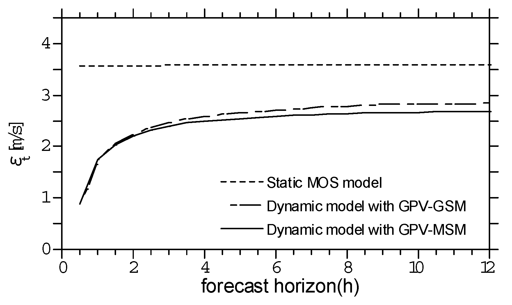
  • The maximum instantaneous wind speed forecast model is constructed using the ARX model. A non-parametric regression with multiple time scale forgetting factors is proposed to identify the model parameters. The maximum instantaneous wind speeds calculated using the proposed dynamic model show favorable agreement with the measurements, whereas the conventional static MOS model underestimates them.
  • The prediction accuracy of the maximum instantaneous wind speed forecast is improved when high-resolution forecast data are used as the input NWP and when multiple time scale forgetting factors are adopted for the proposed dynamic model.
  • The predictability of a strong wind event with a maximum instantaneous wind speed of 15 m/s or more has been evaluated using the ROC curve and the AUC. The proposed dynamic model increases the true positive rate and the AUC increases from 0.84 in the static MOS model to 0.94 in the proposed dynamic model.

Author Contributions

Conceptualization, T.I. and A.Y.; methodology, T.I and A.Y.; software, A.Y.; validation, A.Y.; investigation, A.Y.; data curation, A.Y.; writing—original draft preparation, A.Y.; writing—review and editing, T.I.; visualization, A.Y.; supervision, T.I.; project administration, T.I.; funding acquisition, T.I. All authors have read and agreed to the published version of the manuscript.

Funding

This research received no external funding.

Acknowledgments

This study was conducted as part of the joint research with East Japan Railway Company (JR East) and the University of Tokyo. Yayoi Misu and Yosuke Nagumo of JR East cooperated in providing online measurement data. The authors wish to express their deepest gratitude to the concerned parties.

Conflicts of Interest

The authors declare no conflict of interest.

Appendix A. Non-Parametric Regression with Forgetting Factors

The function ϕ ^ p , t ( q ) , which estimates local q p near the observation at time t so as to minimize the error in Equation (13), is approximated by a quadratic equation in this study. When the vector q is one-dimensional ( Ν = 1 ), the local estimation approximation function ϕ ^ p , t ( q ) can be expressed by the following equation.
ϕ ^ p , t ( q ) = ( ϕ ^ p , t , 1 ( 0 ) + ϕ ^ p , t , 1 ( 1 ) q + ϕ ^ p , t , 1 ( 2 ) q 2 ϕ ^ p , t , 2 ( 0 ) + ϕ ^ p , t , 2 ( 1 ) q + ϕ ^ p , t , 2 ( 2 ) q 2 ϕ ^ p , t , M ( 0 ) + ϕ ^ p , t , M ( 1 ) q + ϕ ^ p , t , M ( 2 ) q 2 )
Estimating the function ϕ ^ p , t ( q ) is equivalent to estimating the coefficient ϕ ^ p , t , m ( l )   ( 0 l 2 ,   0 m M ) . Substituting Equation (A1) into Equation (13), when q is two-dimensional, the error can be written as follows.
ϵ = s = 1 t λ t s w ( q s , q p ) ( y s z s T ϕ ^ p , t ( q ) ) 2
This error ϵ can be calculated as follows.
ϵ = s = 1 t λ t s w ( q s , q p ) [ y s z s T ( ϕ ^ p , t , 1 ( 0 ) + ϕ ^ p , t , 1 ( 1 ) q + ϕ ^ p , t , 1 ( 2 ) q 2 ϕ ^ p , t , 2 ( 0 ) + ϕ ^ p , t , 2 ( 1 ) q + ϕ ^ p , t , 2 ( 2 ) q 2 ϕ ^ p , t , M ( 0 ) + ϕ ^ p , t , M ( 1 ) q + ϕ ^ p , t , M ( 2 ) q 2 ) ] 2
= s = 1 t λ t s w ( q s , q p ) [ y s ( z s , 1 z s , 2 z s , M ) ( ϕ ^ p , t , 1 ( 0 ) + ϕ ^ p , t , 1 ( 1 ) q + ϕ ^ p , t , 1 ( 2 ) q 2 ϕ ^ p , t , 2 ( 0 ) + ϕ ^ p , t , 2 ( 1 ) q + ϕ ^ p , t , 2 ( 2 ) q 2 ϕ ^ p , t , M ( 0 ) + ϕ ^ p , t , M ( 1 ) q + ϕ ^ p , t , M ( 2 ) q 2 ) ] 2
= s = 1 t λ t s w ( q s , q p ) [ y s ( z s , 1 z s , 1 q z s , 1 q 2 z s , M z s , M q z s , M q 2 ) ( ϕ ^ p , t , 1 ( 0 ) ϕ ^ p , t , 1 ( 1 ) ϕ ^ p , t , 1 ( 2 ) ϕ ^ p , t , M ( 0 ) ϕ ^ p , t , M ( 1 ) ϕ ^ p , t , M ( 2 ) ) ] 2
Thus, the error can finally be written as
ϵ = s = 1 t λ t s w ( q s , q p ) ( y s z ˜ s T ϕ ~ p , t ) 2
where
z ˜ s T = ( z s , 1 z s , 1 q z s , 1 q 2 z s , M z s , M q z s , M q 2 ) T , ϕ ˜ p , t = ( ϕ ^ p , t , 1 ( 0 ) ϕ ^ p , t , 1 ( 1 ) ϕ ^ p , t , 1 ( 2 ) ϕ ^ p , t , M ( 0 ) ϕ ^ p , t , M ( 1 ) ϕ ^ p , t , M ( 2 ) ) T
The solution that minimizes ϵ, shown in Equation (A2), can be obtained by Equation (A4) using the least squares method.
ϕ ˜ p , t = ( Z t T Λ t W t , i Z t ) 1 Z t T Λ t W t , i y t
where the matrices Z t , Λ t , W t , i and the vector y t are given by the following equations
Z t = ( z ˜ 1 z ˜ t )
Λ t = ( λ t 1 0 0 λ t t )
W t , i = ( w ( q 1 , q p ) 0 0 w ( q t , q p ) )
y t = ( y 1 y t ) T
Although it is possible to estimate the function by solving Equation (A2) as it is, this requires all the past training data to be stored, which is computationally expensive and inefficient. Instead, recurrence formulae (Equations (A10) and (A11)) have been proposed by using the intermediate matrix R t , i as defined in Equation (A12), which only requires us to store the latest estimation result ϕ ˜ p , t 1 , the latest intermediate matrix R t 1 , i and the newly obtained data.
R t , i = Z t T Λ t W t , i Z t
ϕ ˜ p , t = ϕ ˜ p , t 1 +   w ( q s , q p ) R t , s 1 z t ( y t z t T ϕ ˜ p , t 1 )
R t , i = λ w ( q s , q p ) R t 1 , i + w ( q s , q p ) Z t Z t T
R 0 , i , the initial value of R t , i , has the form shown in Equation (A12):
R 0 , i = ( R 0 0 0 R 0 )
R 0 = 10 was used in this study.

References

  1. Misu, Y.; Ishihara, T. Prediction of frequency distribution of strong crosswind in a control section for train operations by using onsite measurement and numerical simulation. J. Wind Eng. Ind. Aerodyn. 2018, 174, 69–79. [Google Scholar] [CrossRef]
  2. Kobayashi, N.; Shimamura, M. Study of a strong wind warning system. JR East. Tech. Rev. 2003, 2, 61–65. Available online: https://www.jreast.co.jp/e/development/tech/pdf_2/61-65.pdf (accessed on 31 December 2020).
  3. Hoppmann, U.; Koenig, S.; Tielkes, T.; Matschke, G. A short-term strong wind prediction model for railway application: Design and verification. J. Wind Eng. Ind. Aerodyn. 2002, 90, 1127–1134. [Google Scholar] [CrossRef]
  4. Giebel, G.; Landberg, L.; Kariniotakis, G.N.; Brownsword, R. State-of-the-art on methods and software tools for short-term prediction of wind energy production. In Proceedings of the European Wind Energy Conference & Exhibition EWEC, Madrid, Spain, 16–19 June 2003. [Google Scholar]
  5. Giebel, G.; Brownsword, R.; Kariniotakis, G.N.; Denhard, M.; Draxl, C. The State of the Art in Short-Term Prediction of Wind Power: A Literature Overview; ANEMOS.plus: Roskilde, Denmark, 2011. [Google Scholar] [CrossRef]
  6. Landberg, L. Short-Term Prediction of Local Wind Conditions; Risø-R-702(EN); Risø National Laboratory: Roskilde, Denmark, 1994; ISBN 87-550-1916-1. [Google Scholar]
  7. Landberg, L. Short-term prediction of local wind conditions. J. Wind Eng. Ind. Aerodyn. 2001, 89, 235–245. [Google Scholar] [CrossRef] [Green Version]
  8. Sideratos, G.; Hatziargyriou, N.D. An advanced statistical method for wind power forecasting. IEEE Trans. Power Syst. 2007, 22, 258–265. [Google Scholar] [CrossRef]
  9. Soman, S.S.; Zareipour, H.; Malik, O.; Mandal, P. A review of wind power and wind speed forecasting methods with different timehorizons. In Proceedings of the North-American Power Symposium 2010, Arlington, TX, USA, 26–28 September 2010; pp. 1–7. [Google Scholar] [CrossRef]
  10. Giebel, G.; Kariniotakis, G. Wind power forecasting—A review of the state of the art. In Renewable Energy Forecasting: From Models to Applications; Woodhead Publishing: Cambridge, UK, 2017; ISBN 978-0081005040. [Google Scholar]
  11. Dittner, M.E.; Vasel, A. Advances in Wind Power Forecasting. In Advances in Sustainable Energy; Springer: Cham, Switzerland, 2019; ISBN 978-3-030-05635-3. [Google Scholar]
  12. Dhiman, H.S.; Deb, D.; Balas, V.E. Supervised Machine Learning in Wind Forecasting and Ramp Event Prediction; Academic Press: Cambridge, MA, USA, 2020; ISBN 9780128213674. [Google Scholar]
  13. Joensen, A.; Madsen, H.; Nielsen, T.S. Non-parametric Statistical Method for Wind Power Prediction. In Proceedings of the European Wind Energy Conference, Dublin Castle, Ireland, 6–9 October 1997. [Google Scholar]
  14. Pinson, P.; Nielsen, H.A.; Møller, J.K.; Madsen, H.; Kariniotakis, G.N. Non-parametric probabilistic forecasts of wind power: Required properties and evaluation. Wind Energy 2007, 10, 497–516. [Google Scholar] [CrossRef]
  15. Ishizaki, H. Wind profiles, turbulence intensities and gust factors for design in typhoon-prone regions. J. Wind Eng. Ind. Aerodyn. 1983, 13, 55–66. [Google Scholar] [CrossRef]
  16. Saito, K.; Ikawa, M. A numerical study of the local downslope wind “Yamaji-kaze” in Japan. J. Meteorol. Soc. Jpn. 1991, 69, 31–56. [Google Scholar] [CrossRef] [Green Version]
  17. Meng, Z.; Zhang, F. Tests of an ensemble Kalman filter for mesoscale and regional-scale data assimilation. Part III: Comparison with 3DVAR in a real-data case study. Mon. Weather Rev. 2008, 136, 522–540. [Google Scholar] [CrossRef]
  18. Mohrlen, C.; Jorgensen, J. A new algorithm for upscaling and short-term forecasting of wind power using ensemble forecasts. In Proceedings of the 8th International Workshop on Large Scale Integration of Wind Power and on Transmission Networks for Offshore Wind Forms, Bremen, Germany, 14–15 October 2009. [Google Scholar]
  19. Sweats, J.A. Indices of discrimination or diagnostic accuracy: Their ROCs and implied models. Psychol. Bull. 1986, 99, 100–117. [Google Scholar] [CrossRef]
  20. Donaldson, R.J.; Dyer, R.M.; Kraus, M.J. An objective evaluator of techniques for predicting severe weather events. In Proceedings of the 9th Conference on Server Local Storms; American Meteorological Society: Boston, MA, USA, 1975; pp. 321–326. [Google Scholar]
  21. Swets, J.A. Measuring the accuracy of diagnostic systems. Science 1988, 240, 1285–1293. [Google Scholar] [CrossRef] [PubMed] [Green Version]
  22. Kikuchi, Y.; Fukushima, M.; Ishihara, T. Assessment of a coastal offshore wind climate by means of mesoscale model simulations considering high-resolution land use and sea surface temperature data sets. Atmosphere 2020, 11, 379. [Google Scholar] [CrossRef] [Green Version]
  23. Goit, J.P.; Yamaguchi, A.; Ishihara, T. Measurement and prediction of wind fields at an offshore site by scanning Doppler LiDAR and WRF. Atmosphere 2020, 11, 442. [Google Scholar] [CrossRef]
  24. Pinson, P.; Chevallier, C.; Kariniotakis, G.N. Trading Wind Generation from Short-Term Probabilistic Forecasts of Wind Power. IEEE Trans. Power Syst. 2007, 22, 1148–1156. [Google Scholar] [CrossRef] [Green Version]
Figure 1. Overview of the proposed model.
Atmosphere 12 00316 g001
Figure 2. Forecast schedule using GPV-MSM. Each of the three horizontal lines represents distinct product runs initiated from different individual GPV-MSM forecast initializations.
Atmosphere 12 00316 g002
Figure 3. An aerial photograph (a) and elevation contours (b) around the target point.
Atmosphere 12 00316 g003
Figure 4. The function f ( | u ¯ t + k | t nwp | , θ t + k | t nwp ) in the mean wind speed forecast mode: (a)   θ t + k | t nwp = 0 ° ; (b) θ t + k | t nwp = 180 ° .
Atmosphere 12 00316 g004
Figure 5. The training result of a ( k , θ ) and b ( k , θ ) in the mean wind speed forecast model for southerly wind ( θ t + k | t nwp = 180 ° ).
Atmosphere 12 00316 g005
Figure 6. Comparison of measured and forecasted maximum instantaneous wind speeds predicted by the dynamic and conventional static models. The strong wind events as shown from (aj) are listed in Table 2. The strong wind events (a) and (i) were caused by South-coast cyclone, while the other strong wind events were caused by Siberian High and Aleutian Low.
Atmosphere 12 00316 g006
Figure 7. Root mean square error (RMSE) of maximum instantaneous wind speed predicted by the conventional static model output statistics (MOS) and the proposed dynamic models at γ = 0 .
Atmosphere 12 00316 g007
Figure 8. ROC curves of proposed and conventional models.
Atmosphere 12 00316 g008
Figure 9. Difference in dimensionless loss due to difference in γ .
Atmosphere 12 00316 g009
Table 1. Summary of numerical weather prediction data used in this study.
ModelGPV-MSMGPV-GSM (Japan Area)
Forecast horizon39 h84 h
Delivery timeAbout 3 h after initial timeAbout 3 h after initial time
Temporal resolution1 h (surface), 3 h (barometric level)
Initial time (JST)3:00, 9:00, 15:00, 21:003:00, 9:00, 15:00, 21:00
Forecast variablesSea surface rehabilitation pressure (ground surface), altitude (pressure surface), horizontal wind, updraft, temperature, relative humidity, accumulated precipitation
Number of vertical layers60 layers
Horizontal discretization scheme and resolutionGrid point model
resolution: 20 km
Spectrum model
cut-off wave number: 519
Output horizontal grid resolution (surface)0.05 degrees north-south × 0.0625 degrees east-west0.2 degrees north-south × 0.25 degrees east-west
Output Domain22.4° N–47.6° N,
120° E–150° E
20° N–50° N,
120° E–150° E
Table 2. List of targeted strong wind events and corresponding weather conditions
Date and Time
Weather Conditions
Maximum Instantaneous Wind Speed (m/s)Date and Time
Weather Conditions
Maximum Instantaneous Wind Speed (m/s)
2014/01/30 16:00
South-coast cyclone
15.32015/01/31 07:30
Siberian High and Aleutian Low
15.5
2014/01/31 13:00
Siberian High and Aleutian Low
15.62015/02/01 10:00
Siberian High and Aleutian Low
15.0
2014/02/05 10:30
Siberian High and Aleutian Low
15.12015/02/13 15:00
Siberian High and Aleutian Low
15.9
2014/02/16 12:00
Siberian High and Aleutian Low
21.22015/02/15 14:30
Siberian High and Aleutian Low
16.0
2014/03/06 10:30
Siberian High and Aleutian Low
15.32015/02/26 07:30
South-coast cyclone
15.7
2014/03/10 12:30
Siberian High and Aleutian Low
16.22015/02/27 12:30
Siberian High and Aleutian Low
15.7
2014/03/20 06:30
South-coast cyclone
15.72015/03/01 06:00
South-coast cyclone
15.2
2014/03/21 06:30
Siberian High and Aleutian Low
16.22015/03/02 07:00
Siberian High and Aleutian Low
20.1
2014/03/30 10:00
South-coast cyclone
18.82015/03/03 16:30
South-coast cyclone
15.5
2014/03/31 06:00
Siberian High and Aleutian Low
19.42015/03/09 06:00
South-coast cyclone
15.4
2014/12/16 06:30
South-coast cyclone
17.82015/03/10 17:00
Siberian High and Aleutian Low
15.5
2014/12/18 15:30
Siberian High and Aleutian Low
17.62015/12/11 14:30
Siberian High and Aleutian Low
17.4
2014/12/20 07:00
South-coast cyclone
16.32016/01/04 18:00
Siberian High and Aleutian Low
15.9
2015/01/06 15:30
Siberian High and Aleutian Low
17.82016/01/18 06:00
South-coast cyclone
21.8
2015/01/07 07:00
Siberian High and Aleutian Low
16.22016/01/20 07:30
Siberian High and Aleutian Low
17.9
2015/01/17 13:00
Siberian High and Aleutian Low
15.12016/02/09 16:00
Siberian High and Aleutian Low
17.1
2015/01/22 10:30
South-coast cyclone
15.82016/02/10 06:00
Siberian High and Aleutian Low
16.7
2015/01/23 11:30
Siberian High and Aleutian Low
15.12016/03/01 06:00
Siberian High and Aleutian Low
16.8
Table 3. Summary of model parameters.
ParameterValue
Forgetting factor0.917 (peak factor estimation)
0.999 (other than that)
BandwidthWind speed4.0 (m/s)
Wind direction11.25 (deg)
Forecast horizon0.5 (h)
Table 4. Event occurrence table.
Measurement
YesNone
ForecastYesa (True positive)b (False positive)
Nonec (False negative)d (True negative)
Table 5. Area under the curve (AUC) of proposed model and conventional model.
ModelAUC
Static MOS model0.84
Dynamic model with GPV-GSM0.92
Dynamic model with GPV-MSM0.94
Publisher’s Note: MDPI stays neutral with regard to jurisdictional claims in published maps and institutional affiliations.

