Article

Enhancing the Encoding-Forecasting Model for Precipitation Nowcasting by Putting High Emphasis on the Latest Data of the Time Step

1
Department of Data-Centric Problem-Solving Research, Korea Institute of Science and Technology Information (KISTI), Daejeon 34141, Korea
2
Department of Industrial & Systems Engineering, Korea Advanced Institute of Science and Technology (KAIST), Graduate School of Knowledge Service Engineering, Daejeon 34141, Korea
*
Author to whom correspondence should be addressed.
Atmosphere 2021, 12(2), 261; https://doi.org/10.3390/atmos12020261
Submission received: 4 January 2021 / Revised: 7 February 2021 / Accepted: 12 February 2021 / Published: 16 February 2021

Abstract

:
Nowcasting is an important technique for weather forecasting because sudden weather changes significantly affect human life. The encoding-forecasting model, which is a state-of-the-art architecture in the field of data-driven radar extrapolation, does not particularly focus on the latest data when forecasting natural phenomena. This paper proposes a weighted broadcasting method that emphasizes the latest data of the time step to improve the nowcasting performance. This weighted broadcasting method allows the most recent rainfall patterns to have a greater impact on the forecasting network by extending the architecture of the existing encoding-forecasting model. Experimental results show that the proposed model is 1.74% and 2.20% better than the existing encoding-forecasting model in terms of mean absolute error and critical success index, respectively. In the case of heavy rainfall with an intensity of 30 mm/h or higher, the proposed model was more than 30% superior to the existing encoding-forecasting model. Therefore, applying the weighted broadcasting method, which explicitly places a high emphasis on the latest information, to the encoding-forecasting model is considered as an improvement that is applicable to the state-of-the-art implementation of data-driven radar-based precipitation nowcasting.

1. Introduction

With the increase in the number of successful cases of application of deep learning in real life, such as in autonomous driving, healthcare, and smart cities [1,2,3,4,5,6,7,8,9], various attempts have been made to apply deep learning to weather-related fields using numerical models [10] to improve the performance of weather forecasting [11,12,13,14,15]. In the field of meteorology, nowcasting is a popular research topic in which deep learning techniques are being actively applied to the analysis of spatiotemporal data, such as radar and satellite data [16,17,18,19].
Precipitation nowcasting is the prediction of the spatiotemporal distribution of rainfall that will occur within a relatively short period of time. It is a very important weather forecasting technique for securing a golden time in natural disasters, such as flooding caused by sudden torrential rain. The extant nowcasting methods can be classified into traditional methods based on numerical models or optical flows and machine learning methods based on statistical methods [19]. In the past, optical flow methods were mainly employed because numerical models required a long initial driving time. Nevertheless, in recent years, deep learning using statistical methods is being actively studied because it surpasses traditional methods in performance [19,20,21].
A deep learning-based nowcasting method can be defined as a spatiotemporal sequence prediction problem that inputs a sequence of past observation data and outputs a sequence of future changed patterns. Deep learning-based methods are further divided into image-to-image translation problems using only convolutional neural network (CNN) and sequence-to-sequence problems using recurrent neural network (RNN) that explicitly model temporal phenomena [19]. Because models using only CNN do not explicitly model temporal phenomena, unlike RNN, the following two methods are used to predict future time steps. The first method predicts a single step in the future using CNN and uses the predicted result again as an input to predict the next step repeatedly [22]. The second method predicts the output channel of the CNN after changing the time of the RNN to the channel of the CNN [21]. U-Net architecture is mainly used in the CNN-based methods [19,22,23,24], and stacked convolutional RNN architecture is mainly used in the RNN-based methods [20,21,25,26]. Shi et al. [20,21] conducted experiments comprehensively on various methods such as optical flow, 2D CNN, 3D CNN, RNN, and a method of combining CNN and RNN. Among them, the encoding-forecasting model in which CNN and RNN were repeatedly stacked showed the best performance.
With the success of the encoding-forecasting model, several follow-up studies have been conducted to further improve the performance of the model. Most of these studies are related to model optimization such as tuning hyperparameters or creating an ensemble model. Tran and Song [18] combined the structural similarity index used to measure the image quality and distance-based loss functions such as mean absolute error (MAE) and mean square error (MSE) to improve the existing model. In addition, they decreased the number of channels in high abstract recurrent layers, unlike the usual methods. Franch et al. [27] improved the prediction performance of extreme events by creating an ensemble model based on the existing model. Tran and Song [16] improved the model performance by introducing a data augmentation technique to RNN as in CNN. Although the encoding-forecasting model [20,21,26] is currently showing the best performance, it still overlooks the fact that data of the latest phenomena should be considered more heavily when forecasting natural phenomena.
By extending the architecture, this study seeks to overcome the shortcomings of the encoding-forecasting model, which is a state-of-the-art architecture in the field of radar echo extrapolation and nowcasting [21]. To achieve this goal, we propose an improved deep learning model incorporating a weighted broadcasting block that explicitly reflects the latest phenomena. Weighted broadcasting involves transferring the latest feature map generated from the convolutional layers of the encoding network to the deconvolutional layers of the forecasting network using skip connection and applying different weights for each time step of the forecasting network. Using the weighted broadcasting method that deploys skip connection, the vanishing gradient problem occurring in the encoding-forecasting model can be alleviated. Herein, the superior performance indices, such as distance and confusion metrics, of the weighted broadcasting-based encoding-forecasting model were confirmed by comparing them with those of the existing encoding-forecasting model.

2. Data and Methods

This section explains the construction of the dataset for training and evaluation, and the details of the proposed model.

2.1. Dataset

Weather radar data reflecting the seasonal characteristics of the Korean Peninsula during the torrential downpour period in summer from June to September for the period of 2012 to 2017 were used to construct the dataset. This study used the constant altitude plan position indicator (CAPPI) 1.5 km data provided by the Korea Weather Radar Center, which represents the horizontal cross-section of data at a constant altitude of 1.5 km, measured using the volume scans of 11 weather radars (GDK, BRI, GNG, IIA, KWK, KSN, MYN, PSN, JNI, GSN, and SSP) operated by the Korea Meteorological Administration. A Lambert conformal conic projection was applied to the CAPPI, and a dataset was constructed using 256 × 256 grids with a horizontal resolution of 2 km. Because the CAPPI provides reflectivity (unit: dBZ), the Z-R relationship [28], which is used to convert reflectivity to the intensity of rainfall as shown below, was applied to obtain the rainfall rate for every 10 min.
R   = ( 10 Z 10 200 ) 5 3  
where R is rainfall rate ( mm   h 1 ) and Z is reflectivity ( dBZ ).
Furthermore, the input values were rescaled to (0,1) through the min-max normalization using the range of 0 mm/h (minimum) to 110 mm/h (maximum) during data preprocessing. Of the entire dataset, odd-numbered days from 2012 to 2017 were used as training data, and even-numbered days were used as the validation and test sets. From the even-numbered days, even-numbered months of even-numbered years and odd-numbered months of odd-numbered years were used as the validation set, whereas the odd-numbered months of even-numbered years and even-numbered months of odd-numbered years were used as the test set. By configuring the data as such, the training, validation, and test datasets showed a similar distribution.
The final configuration of the datasets is as listed in Table 1.
For the experiment of the encoding-forecasting model, we prepared an experimental environment for nowcasting that forecasts rainfall 3 h in the future after observing 3 h of past data. With a temporal resolution of 10 min, the time-step lengths of both the input and output sequences of the model were 18 each. Therefore, the total time-step length of a single data instance comprising input and output sequence was 36 (18+18).
Because of the nature of rainfall (i.e., it does not often rain all day long), a vast amount of training data was composed of sequences without rainfall. Figure 1 shows the distribution of the training data by rainfall intensity. As shown, the data distribution is concentrated at a rainfall intensity of 0.8 or below. When the model is trained in this state, the model may be trained with the bias toward the periods without rainfall. To address this issue, this study trained the model using only the data for which the average rainfall intensity of a data instance comprising 36 × 256 × 256 grids was 0.8 or higher. In this way, the problem of uneven distribution of rainfall data was mitigated for the training process.
Finally, after filtering the data of each category with a rainfall intensity threshold of 0.8, 3335 training sequences, 2321 validation sequences, and 1894 testing sequences were used as sequence samples.

2.2. Proposed Model

The weighted broadcasting (WB) based encoding-forecasting model proposed in this study is a model optimized for nowcasting a relatively short term of approximately 3–6 h in the near future. To improve the performance of the existing encoding-forecasting model, the concept of weighted broadcasting block (WB-Block), which emphasizes the latest data in the time step from past observations, is introduced. In addition, we combine the WB-Block with the convolutional layer of the encoding-forecasting model to improve nowcasting performance.

2.2.1. Preliminaries

  • ConvLSTM Cell
The convolutional long short-term memory (ConvLSTM) cell is the most commonly used method for spatiotemporal sequence modeling because it can perform simultaneous spatiotemporal analysis [20]. The ConvLSTM cell achieves stable and powerful spatiotemporal modeling performance by combining the long-range temporal dependence analysis of the existing long short-term memory (LSTM) [29] and the spatial characteristic analysis capability of the CNN.
The key formulas of each module constituting the ConvLSTM cell are shown in Equation (2):
i t   =   σ ( W xi     Χ t +   W hi     H t 1 +   W ci   C t 1 +   b i ) f t   =   σ ( W xf     Χ t +   W hf     H t 1 +   W cf   C t 1 +   b f ) C t   =   f t   C t 1 +   i t tan h ( W xc     Χ t +   W hc     H t 1 +   b c ) o t   =   σ ( W xo     Χ t +   W ho     H t 1 +   W co   C t +   b o ) H t   =   o t tan h ( C t ) :   convolution   operator ,   o :   Hadamard   product
H t , C t , and X t represent the short-term state, long-term state, and input value, respectively. f t ,     i t , and o t are used to control the state and input value. More specifically, f t controls the part of the long-term state that should be erased. i t controls the part of the input value that should be added to the long-term state. o t controls the part of the long-term state that should be read and output as the result of the current time step. W and b denote the weight matrix and bias, respectively. Finally, σ and tan h represent the sigmoid and hyperbolic tangent function, respectively.
  • Encoding-forecasting model
The encoding-forecasting model employs a sequence-to-sequence (seq2seq)-based network structure [30], which combines an encoding network and a forecasting network to address the spatiotemporal sequence forecasting problem. The encoding network analyzes spatiotemporal patterns of past data to generate latent vectors, and the forecasting network uses latent vectors of the encoding network to forecast future rainfall. In general, the encoding network is constructed by stacking a convolutional layer, which performs downsampling and spatial abstraction, and a recurrent layer, which compresses temporal patterns. The forecasting network is constructed by stacking a deconvolutional layer, which performs upsampling and spatial concretization, and a recurrent layer, which predicts future patterns from compressed temporal patterns.

2.2.2. Model Description

This study proposes a model that combines the weighted broadcasting and the encoding-forecasting model to improve the performance of nowcasting. The architecture of the proposed model is shown in Figure 2, where (A × A, B) denotes the output of the layer constituting the network, e.g., (128 × 128, 16), (64 × 64, 32), (32 × 32, 64). The symbols A and B denote the size and number of channels, respectively, of the resulting feature map, whereas k and s in the convolutional layer represent the size of the kernel and stride, respectively.
Before examining the proposed model, it must be noted that the convolutional and recurrent layers are stacked repeatedly in the encoding and forecasting part of the existing encoding-forecasting model. While the shallow convolutional layers capture the regional and detailed features of the spatial distribution of precipitation, the deeper convolutional layers capture the global and abstracted features; this is the most significant characteristic of the convolutional layer. In addition, the recurrent layers between the convolutional layers analyze the past rainfall patterns over time at each level abstracted by the convolutional layers; this is the most significant characteristic of the recurrent layer. The rainfall pattern information analyzed in each recurrent layer at each abstraction level of the encoding network is transferred to the recurrent layer corresponding to the concretization level of the forecasting network for prediction of the future rainfall pattern. At this stage, the output information of the deconvolutional layer at each concretization level constituting the forecasting network is combined to supplement the information generated from the previous concretization level.
In this study, the performance of the existing encoding-forecasting model is improved by applying a WB-Block, which puts more weight on the most recent feature map in the convolutional layer of the encoding network. While predicting future rainfall, patterns of past observations are analyzed, and the most recent rainfall patterns have the greatest influence on future patterns. Therefore, when predicting the output radar R’t+1 ~ R’t+n using the input radar data Rt-m+1 ~ Rt, the module in Figure 3 is added to reflect the feature map of the t-th time step of the encoding network with greater importance. Essentially, in the encoding-forecasting model, the recurrent layers of the encoding network and the forecasting network are combined using a state copy to generate the structure of the seq2seq model. Hence, m and n, which are the sequence lengths of the encoding network and the forecasting network, can be different from each other. Figure 3 shows that the WB-Block broadcasts feature maps of the last time step of the convolutional layer of the encoding network to all the time steps of the corresponding deconvolutional layer of the forecasting network. During the process, as the time step of the forecasting network incrementally increases from t + 1 to t + n, the influence of the feature map at the t-th time step of the encoding network decreases. The weight change that occurs as the time step increases is desirable. The influence of the feature maps at the t-th time step should decrease as the effect of a current event decreases over time. In general, the influence decreases as the time step increases; however, the reduction is not constant across the time steps. Therefore, the model should learn these patterns through the data while adjusting the weights to reflect the natural phenomena represented in the training data. In addition, because weight variables, represented as W = (wt+1, wt+2, wt+3, …, wt+n-2, wt+n-1, wt+n) in Figure 3, are shared during training through all convolutional layers, there is little overhead for computation and memory usage. When the time step increases and the effect of weight decreases, the influence of the latest feature map of the encoding network is reduced, and the feature map transmitted from the previous recurrent layer of the forecasting network is used with relatively higher importance to perform prediction. Unlike the existing encoding-forecasting model, the number of input channels is doubled in the deconvolutional layer of the forecasting network. Through weighted broadcasting, the feature map is transferred to the forecasting network via skip connection represented as a feature map concatenation in Figure 2. The channel is temporarily doubled at the input of each deconvolutional layer and then reduced to half at the output of the deconvolutional layer. In other words, in the first deconvolutional layer of the forecasting network the input channel is 128 and the output channel is 64, and the input and output channels in the second deconvolutional layer become 64 and 32, respectively. In the third deconvolutional layer, the input and output channels are 32 and 16, respectively.

2.3. Experimental Setup and Evaluation Metrics

2.3.1. Experimental Setup

Based on the constructed dataset, experiments using the proposed model and comparison model were repeated 10 times each. The numerical values presented in this section represent the average values of the results of 10 experiments. We used NVIDIA Tesla P100 GPU (×2) and Google TensorFlow 2.1 version for the experiment, and for multi-GPU learning, the “NcclAllReduce” option was used as TensorFlow’s MirroredStrategy. It took approximately 8 h per experiment. Adam [31] was used as the optimization algorithm of the neural network, and Adam’s learning_rate, beta_1, beta_2, and epsilon were set to 0.0001, 0.9, 0.999, and 1 × 10⁻⁷, respectively. In addition, “glorot_uniform,” “orthogonal,” and “zeros” were used for kernel_initializer, recurrent_initializer, and bias_initializer of cells used, respectively. Considering the high-resolution radar data, the batch size was set to 4, and batch normalization was used as a regularization technique. MSE was used as the loss function, and early stopping [32] was adapted to terminate training when no improvement in validation loss was observed within 10 epochs.

2.3.2. Evaluation Metrics

To evaluate the performance of the proposed model, we present a distance-based metric, which is a basic measure of reconstruction evaluation, and a confusion matrix-based metric, for evaluation based on rainfall intensity.
First, the distance-based metrics include the MAE, MSE, and balanced MSE (B-MSE) [21]. B-MSE, adopted from Shi et al. [21], has a feature that applies a greater loss penalty as the rainfall level increases, reflecting the intensity of damage to humans. The distance-based metrics do not classify rainfall by level but they calculate the mean error between the predicted value and ground truth for all cases from light to heavy rainfall. Therefore, these metrics are used to compare the overall performance of the model for all categories of rainfall rather than to compare the performance of the model according to the rainfall levels. The equations used to calculate the metric values are as follows:
MAE   =   n = 1 N t = 1 T i = 1 I j = 1 J | p prediction ( n , t , i , j ) p ground   truth ( n , t , i , j ) | N   ×   T   ×   I   ×   J
MSE   =   n = 1 N t = 1 T i = 1 I j = 1 J ( p prediction ( n , t , i , j ) p ground   truth ( n , t , i , j ) ) 2 N   ×   T   ×   I   ×   J
B - MSE   =   n = 1 N t = 1 T i = 1 I j = 1 J w ( n , t , i , j )   ×   ( p prediction ( n , t , i , j ) p ground   truth ( n , t , i , j ) ) 2 N   ×   T   ×   I   ×   J
In the equations, N, T, I, and J represent the number of test samples, the length of the future time step, the height of the 2D prediction space, and the width of the 2D prediction space, respectively. Table 2, which is adopted from Shi et al. [21], summarizes the weight of the loss penalty according to the level of the rainfall rate when computing the B-MSE.
Next, the false alarm rate (FAR), possibility of detection (POD), critical success index (CSI), and the Heidke skill score (HSS) [33] were obtained using the following formulas based on the confusion matrix presented in Table 3. A method of measuring prediction performance according to the level of rainfall rate based on the confusion matrix, which is used in a classification problem, is a common method in the meteorological field [16,18,20,21,24,25,27]. After predicting rainfall through the model, we generate five confusion matrices based on the five thresholds (i.e., the rainfall rate of 0.5, 2.0, 5.0, 10.0, and 30.0 mm/h). We create each confusion matrix by converting the predicted value and ground truth to 1 if they are above the threshold and 0 otherwise. The confusion matrix-based metrics are useful for subdividing and evaluating rainfall by level. In other words, it is possible to determine in detail whether the model’s predictive performance is excellent in heavy rainfall or light rainfall.
FAR   =   FP TP   +   FP
POD   =   TP TP   +   FN
CSI   =   TP TP   +   FP   +   FN
HSS   =   TP TN FN FP ( TP   +   FN ) ( FN   +   TN )   +   ( TP   +   FP ) ( FP   +   TN )

3. Results

Table 4 summarizes the results of the distance-based performance metrics obtained from the experiment. The values in Table 4 were calculated using the values between 0 and 1, rescaled through the min-max normalization of 0 mm/h to 110 mm/h.
In the distance-based performance metrics, a lower value indicates better performance. Although the MSE of the WB-based encoding-forecasting model is slightly worse (−0.25%), the MAE (+1.74%) and B-MSE (+1.08%) indicate that the proposed model is superior to the existing encoding-forecasting model.
Next, the results of the performance metrics based on the confusion matrix are presented in Table 5 and Table 6.
In the FAR and POD performance metrics in Table 5, FAR shows the proportion of poorly predicted items among predicted items; hence, the lower the value, the better the performance. POD, on the other hand, represents the ratio of the items that are properly detected among the items to be detected; thus, the higher the value, the better the performance. These two are performance indicators that have a trade-off relationship with each other. As one value improves, the other value tends to deteriorate. As shown in Table 5, the proposed model has excellent detection capability in heavy rainfall.
In the CSI and HSS performance metrics in Table 6, a higher value indicates better performance. Here, CSI is an index that represents comprehensive performance evaluation by expressing the performance of FAR and POD as one metric. For all five categories of rainfall intensity, the proposed model using weighted broadcasting exhibits superior performance. In particular, the proposed model using weighted broadcasting shows more than 30% improved performance in CSI metric than the existing model when the rainfall intensity is 30 mm/h or higher, which is the intensity value when the influence of rainfall on human life becomes substantial, implying that the proposed model can be useful for applications such as flood prediction [34,35,36].
Figure 4 shows the CSI and HSS scores of the two compared models while varying the future time steps. As can be observed in the figure, the proposed model is superior to the existing model especially in the cases of rainfall with an intensity of 5, 10, and 30 mm/h. The comparisons for the other metrics corresponding to the future time steps are presented in Figure A1 and Figure A2 (Appendix A).
As a final step in the quantitative performance evaluation, a Monte Carlo permutation test [37] was performed to assess whether the quantitative performance metrics had significant differences between the two models (see Table A1, Appendix B for details). The Monte Carlo permutation test is a statistical method for testing whether there is a significant difference between two groups even when the underlying distribution is unknown. The Monte Carlo permutation test showed significant differences for 20 metrics out of the 23 metrics examined in this study, indicating that the differences between the two models were predominantly significant. For only MSE, B-MSE, and HSS-30.0, the p-value was higher than 0.05.
Apart from the quantitative evaluation metrics, examples of the actual input frames and prediction frames for qualitative evaluation that can be interpreted by human visual perception are presented in Figure 5 and Figure 6. Figure 5 shows an example of 18 radar observation frames used as inputs, and Figure 6 shows the prediction frames of the two comparison models (the encoding-forecasting model and WB-based encoding-forecasting model) and the actual ground truth frames.
As shown in Figure 6, particularly the predicted frames from time steps t + 3 to t + 8, the existing encoding-forecasting model shows that the shape of the heavy rainfall rate is elongated, whereas the WB-based encoding-forecasting model shows that the shape of the heavy rainfall rate is similar to that of the ground truth. In addition, the predicted frames from time steps t + 13 to t + 18 demonstrate that the existing model shows a separation of the shape of heavy rainfall rate, whereas the proposed model shows a shape similar to that of the ground truth. However, both models show that the results are smoothed to the predictable scales overall. In addition, there is not only loss of variance, but also reduction of precipitation. Nevertheless, we can summarize that the WB-based encoding-forecasting model shows better performance than that of the existing encoding-forecasting model, following more closely the shape of the ground truth.
Figure 7 shows the learned weight values of the WB-based encoding-forecasting model. As mentioned earlier, the model using the WB-Block is designed to learn the weight on its own according to the provided input data. The values of the weights obtained after going through 10 experiments are shown in gray line, and the average weight values are shown in blue line.
As shown in Figure 7, data at time step t, the most recent rainfall pattern, has a stronger effect at the beginning of the future prediction; however, its effect gradually decreases as it moves to the later time steps. This pattern indicates that when information delivered from the convolutional layers of the encoding network is used in the corresponding deconvolutional layers of the forecasting network, it has different weights and influences according to the future time step. In the later part of the time step where the weight value is decreased, the feature map transferred from the recurrent layer of the forecasting network is used more heavily. The values of the weights were not manually set by humans; rather, they were learned by the model as it found an appropriate value according to the characteristics of the data.

4. Conclusions

In this study, we proposed a WB-based encoding-forecasting model that improves the performance of nowcasting by applying weighted broadcasting, which emphasizes the influence of the latest feature map of the observed data in the encoding-forecasting model. Through experiments, this study verified that the nowcasting approach based on the proposed model exhibits superior performance in many aspects compared with the existing encoding-forecasting model. The findings clearly indicate that applying the weighted broadcasting method that explicitly places more emphasis on the latest information in the convolutional layer, in addition to the pattern analysis over time implicitly performed in the recurrent layer, to the encoding-forecasting model improves nowcasting performance. The reason weighted broadcasting can improve the performance of nowcasting is that it obtains and uses important information that could not be analyzed through the recurrent layers alone. This combinatory approach proves that, when predicting the sequence of natural phenomena, the phenomenon of the last data transmitted through weighted broadcasting is crucial.
However, the limitations that can occur in this prediction schema are as follows. When making a prediction in a section in which the rainfall radar pattern changes in an instant, the past and future patterns may be completely different. In that case, the effect of weighted broadcasting may be limited. However, even in such a case, the model can still be adequate because the weight variable is adjusted according to the data during training, which automatically reduces the influence of information from the convolutional layers of the encoding network and increases the influence of the information from the recurrent layers of the forecasting network. At least, it does not limit the performance of the existing encoding-forecasting model. Therefore, weighted broadcasting can be used in combination with the encoding-forecasting model at any time. To calculate the weights of weighted broadcasting, only additional trainable variables equal to the length of the future time steps are needed.
In this study, when supplementing information missing from the recurrent layer of the existing encoding-forecasting model through weighted broadcasting of the convolutional layer, only the last feature map on the past time step of the convolutional layer was used. However, because useful information can be found not only in the last feature map but also in the previous feature map even if the probability is small, it may be further improved by applying the self-attention technique [38] to the feature map to extract and utilize selectively the most important feature map. We plan to explore this idea in our future research.

Author Contributions

Conceptualization, C.H.J. and M.Y.Y.; methodology, C.H.J.; software, C.H.J.; validation, M.Y.Y.; formal analysis, D.J. and W.K.; investigation, D.J.; resources, W.K.; data curation, W.K. and D.J.; writing—original draft preparation, C.H.J.; writing—review and editing, C.H.J. and M.Y.Y.; visualization, W.J.; supervision, M.Y.Y.; project administration, W.J.; funding acquisition, W.J. All authors have read and agreed to the published version of the manuscript.

Funding

This research was supported by Ministry of Science, ICT, Republic of Korea (Project No. K-21-L01-C05-S01).

Institutional Review Board Statement

Not applicable.

Informed Consent Statement

Not applicable.

Data Availability Statement

Publicly available datasets were analyzed in this study. This data can be found here: https://data.kma.go.kr/data/rmt/rmtList.do?code=11&pgmNo=62 (accessed on 15 February 2021).

Conflicts of Interest

The authors declare no conflict of interest.

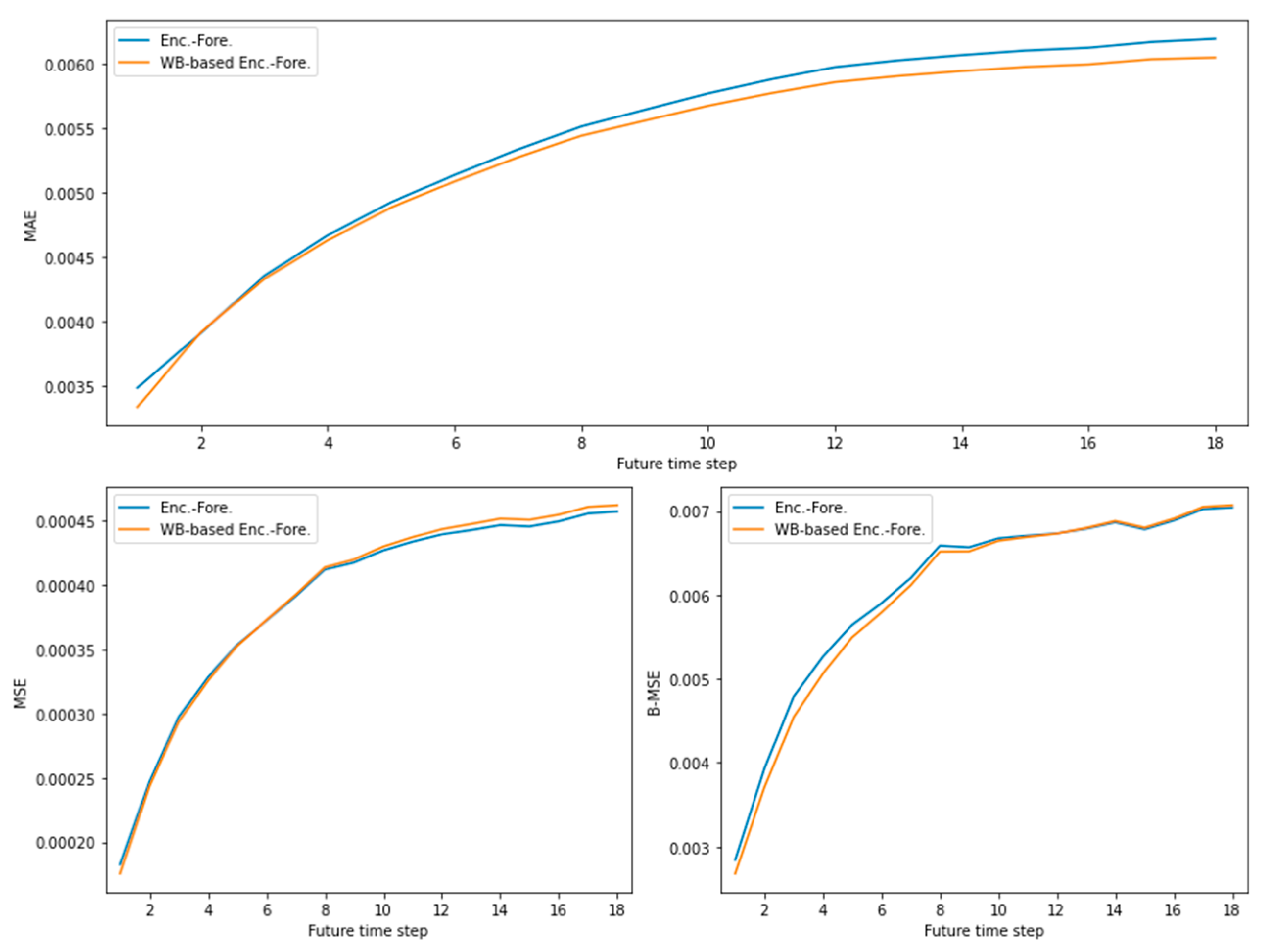
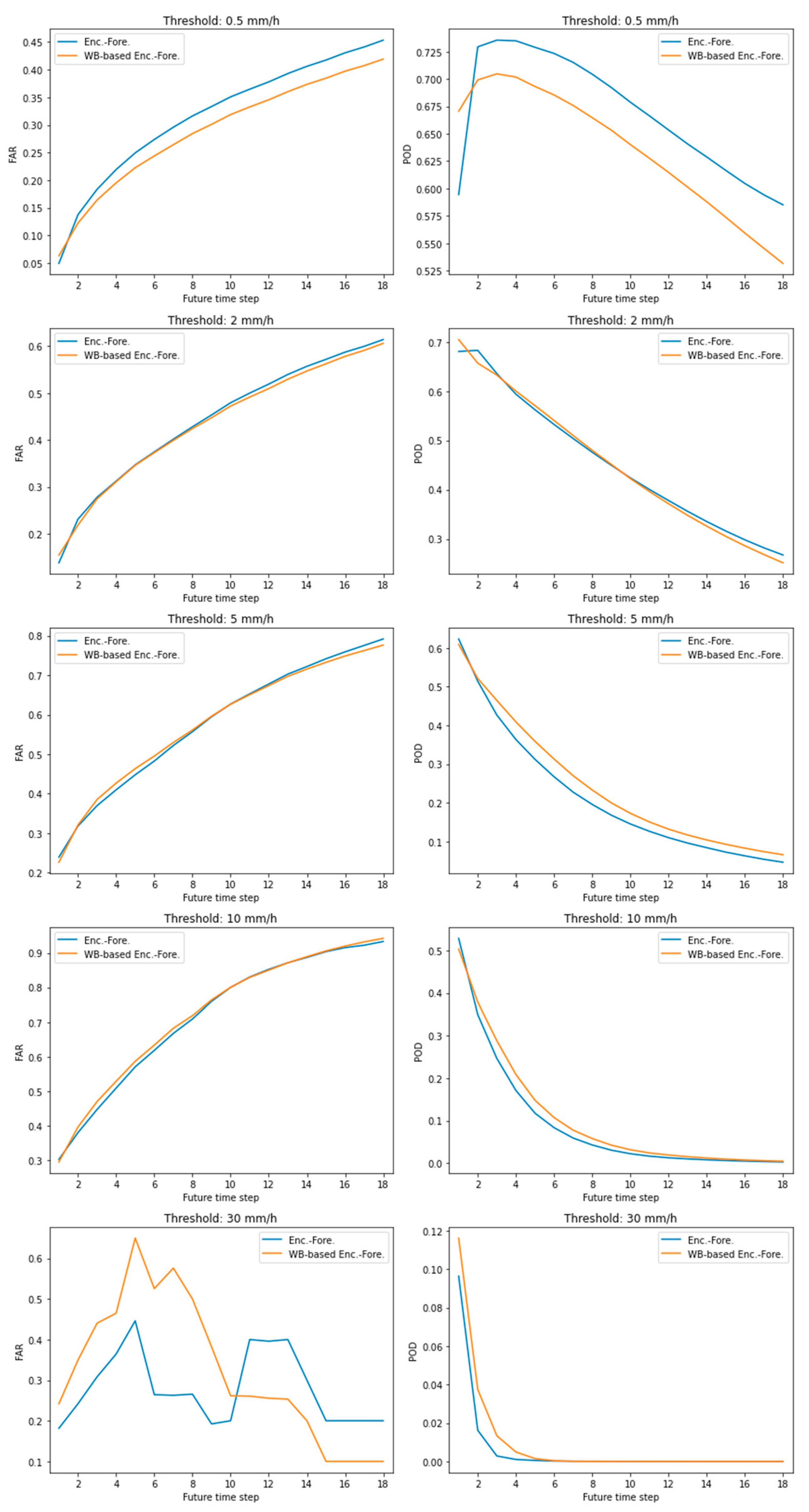
Appendix A. Model Comparison According to the Future Time Step

Figure A1 shows the model comparisons for distance-based metrics, such as MAE, MSE, and B-MSE, across the future time steps. As shown in Figure A1, the WB-based encoding-forecasting model is slightly worse than the existing encoding-forecasting model, in terms of MSE. However, the WB-based encoding-forecasting model is better than the existing model in terms of MAE and B-MSE. In addition, when we compare the models in terms of the MAE, which indicates the simple difference of the error, it can be observed that the WB-based encoding-forecasting model gradually performs better as the future time step increases.
Figure A1. MAE, MSE, and B-MSE comparison of the proposed model and the existing model across the future time steps.
Atmosphere 12 00261 g0a1
Figure A2 shows the model comparisons for the confusion matrix-based metrics, such as FAR and POD, across the future time steps. FAR and POD are performance indicators that have a trade-off relationship with each other. As shown in Figure A2, the existing model has better detection ability in light rainfall intensity such as 0.5 and 2 mm/h; however, the WB-based encoding-forecasting model has better detection ability in heavy rainfall intensity such as 5, 10, and 30 mm/h.
Figure A2. FAR and POD comparison of the proposed model and the existing model across the future time steps.
Atmosphere 12 00261 g0a2

Appendix B. Monte Carlo Permutation Test

Table A1. P-values of the Monte Carlo permutation tests.
Metricp-Value
(Lower B
ound)
p-Value
(Upper Bound)
Significance
MAE0.01270488650510270.0174676687141277O
MSE0.38874585374814370.4079322515204518X
B-MSE0.36963911680579830.3886537340002310X
FAR-0.50.00.0006630497334598O
FAR-2.00.00.0006630497334598O
FAR-5.00.00.0006630497334598O
FAR-10.00.00.0006630497334598O
FAR-30.00.00.0006630497334598O
POD-0.50.00.0006630497334598O
POD-2.00.00.0006630497334598O
POD-5.00.00.0006630497334598O
POD-10.00.00.0006630497334598O
POD-30.00.00.0006630497334598O
CSI-0.50.00.0006630497334598O
CSI-2.00.00.0006630497334598O
CSI-5.00.00.0006630497334598O
CSI-10.00.00372981957954610.0075262018267390O
CSI-30.00.02072998529109590.0287007076153710O
HSS-0.50.00.0006630497334598O
HSS-2.00.00.0006630497334598O
HSS-5.00.00.0006630497334598O
HSS-10.00.00.0006630497334598O
HSS-30.00.17061054676060140.1904134072389727X

References

  1. Munoz-Organero, M.; Ruiz-Blaquez, R.; Sánchez-Fernández, L. Automatic detection of traffic lights, street crossings and urban roundabouts combining outlier detection and deep learning classification techniques based on GPS traces while driving. Comput. Environ. Urban Syst. 2018, 68, 1–8. [Google Scholar] [CrossRef] [Green Version]
  2. Huval, B.; Wang, T.; Tandon, S.; Kiske, J.; Song, W.; Pazhayampallil, J.; Andriluka, M.; Rajpurkar, P.; Migimatsu, T.; Cheng-Yue, R.; et al. An Empirical Evaluation of Deep Learning on Highway Driving. arXiv 2015, arXiv:1504.01716. [Google Scholar]
  3. Grigorescu, S.; Trasnea, B.; Cocias, T.; Macesanu, G. A survey of deep learning techniques for autonomous driving. J. Field Robot. 2020, 37, 362–386. [Google Scholar] [CrossRef]
  4. Esteva, A.; Robicquet, A.; Ramsundar, B.; Kuleshov, V.; Depristo, M.; Chou, K.; Cui, C.; Corrado, G.; Thrun, S.; Dean, J. A guide to deep learning in healthcare. Nat. Med. 2019, 25, 24–29. [Google Scholar] [CrossRef] [PubMed]
  5. Faust, O.; Hagiwara, Y.; Hong, T.J.; Lih, O.S.; Acharya, U.R. Deep learning for healthcare applications based on physiological signals: A review. Comput. Methods Programs Biomed. 2018, 161, 1–13. [Google Scholar] [CrossRef] [PubMed]
  6. Purushotham, S.; Meng, C.; Che, Z.; Liu, Y. Benchmarking deep learning models on large healthcare datasets. J. Biomed. Informatics 2018, 83, 112–134. [Google Scholar] [CrossRef]
  7. Chen, Q.; Wang, W.; Wu, F.; De, S.; Wang, R.; Zhang, B.; Huang, X. A Survey on an Emerging Area: Deep Learning for Smart City Data. IEEE Trans. Emerg. Top. Comput. Intell. 2019, 3, 392–410. [Google Scholar] [CrossRef] [Green Version]
  8. Wang, L.; Sng, D. Deep Learning Algorithms with Applications to Video Analytics for A Smart City: A Survey. arXiv 2015, arXiv:1512.03131. [Google Scholar]
  9. Mohammadi, M.; Al-Fuqaha, A.; Guizani, M.; Oh, J.-S. Semisupervised Deep Reinforcement Learning in Support of IoT and Smart City Services. IEEE Internet Things J. 2017, 5, 624–635. [Google Scholar] [CrossRef] [Green Version]
  10. Skamarock, W.C.; Klemp, J.B.; Dudhia, J.; Gill, D.O.; Barker, D.M.; Duda, M.G.; Huang, X.-Y.; Wang, W.; Powers, J.G. A Description of the Advanced Research WRF Version 3. Available online: https://opensky.ucar.edu/islandora/object/technotes:500 (accessed on 15 February 2021).
  11. Banadkooki, F.B.; Ehteram, M.; Ahmed, A.N.; Fai, C.M.; Afan, H.A.; Ridwam, W.M.; Sefelnasr, A.; El-Shafie, A. Precipitation Forecasting Using Multilayer Neural Network and Support Vector Machine Optimization Based on Flow Regime Algorithm Taking into Account Uncertainties of Soft Computing Models. Sustainability 2019, 11, 6681. [Google Scholar] [CrossRef] [Green Version]
  12. Nourani, V.; Uzelaltinbulat, S.; Sadikoglu, F.; Behfar, N. Artificial intelligence based ensemble modeling for multi-station prediction of precipitation. Atmosphere 2019, 10, 80. [Google Scholar] [CrossRef] [Green Version]
  13. Anh, D.T.; Dang, T.D.; Van, S.P. Improved Rainfall Prediction Using Combined Pre-Processing Methods and Feed-Forward Neural Networks. J. Multidiscip. Res. 2019, 2, 65–83. [Google Scholar]
  14. Benevides, P.; Catalao, J.; Nico, G. Neural Network Approach to Forecast Hourly Intense Rainfall Using GNSS Precipitable Water Vapor and Meteorological Sensors. Remote Sens. 2019, 11, 966. [Google Scholar] [CrossRef] [Green Version]
  15. Poornima, S.; Pushpalatha, M. Prediction of Rainfall Using Intensified LSTM Based Recurrent Neural Network with Weighted Linear Units. Atmosphere 2019, 10, 668. [Google Scholar] [CrossRef] [Green Version]
  16. Tran, Q.-K.; Song, S.-K. Multi-ChannelWeather Radar Echo Extrapolation with Convolutional Recurrent Neural Networks. Remote Sens. 2019, 11, 2303. [Google Scholar] [CrossRef] [Green Version]
  17. Wehbe, Y.; Temimi, M.; Adler, R.F. Enhancing Precipitation Estimates Through the Fusion of Weather Radar, Satellite Retrievals, and Surface Parameters. Remote Sens. 2020, 12, 1342. [Google Scholar] [CrossRef] [Green Version]
  18. Tran, Q.-K.; Song, S.-K. Computer Vision in Precipitation Nowcasting: Applying Image Quality Assessment Metrics for Training Deep Neural Networks. Atmosphere 2019, 10, 244. [Google Scholar] [CrossRef] [Green Version]
  19. Agrawal, S.; Barrington, L.; Bromberg, C.; Burge, J.; Gazen, C.; Hickey, J. Machine Learning for Precipitation Nowcasting from Radar Images. arXiv 2019, arXiv:1912.12132. [Google Scholar]
  20. Shi, X.; Chen, Z.; Wang, H.; Yeung, D.-Y.; Wong, W.; Woo, W. Convolutional LSTM Network: A Machine Learning Approach for Precipitation Nowcasting. In Advances in Neural Information Processing Systems 28; Cortes, C., Lawrence, N.D., Lee, D.D., Sugiyama, M., Garnett, R., Eds.; Curran Associates, Inc.: Red Hook, NY, USA, 2015; pp. 802–810. [Google Scholar]
  21. Shi, X.; Gao, Z.; Lausen, L.; Wang, H.; Yeung, D.Y.; Wong, W.K.; Woo, W.C. Deep Learning for Precipitation Nowcasting: A Benchmark and A New Model. In Advances in Neural Information Processing Systems 30; Guyon, I., Luxburg, U.V., Bengio, S., Wallach, H., Fergus, R., Vishwanathan, S., Garnett, R., Eds.; Curran Associates, Inc.: Red Hook, NY, USA, 2017; pp. 5617–5627. [Google Scholar]
  22. Ayzel, G.; Scheffer, T.; Heistermann, M. RainNet v1.0: A convolutional neural network for radar-based precipitation nowcasting. Geosci. Model Dev. 2020, 13, 2631–2644. [Google Scholar] [CrossRef]
  23. Lebedev, V.; Ivashkin, V.; Rudenko, I.; Ganshin, A.; Molchanov, A.; Ovcharenko, S.; Grokhovetskiy, R.; Bushmarinov, I.; Solomentsev, D. Precipitation Nowcasting with Satellite Imagery. In Proceedings of the 25th ACM SIGKDD International Conference on Knowledge Discovery & Data Mining, Anchorage, AK, USA, 4–8 August 2019; pp. 2680–2688. [Google Scholar]
  24. Ayzel, G.; Heistermann, M.; Sorokin, A.; Nikitin, O.; Lukyanova, O. All convolutional neural networks for radar-based precipitation nowcasting. Procedia Comput. Sci. 2019, 150, 186–192. [Google Scholar] [CrossRef]
  25. Kumar, A.; Islam, T.; Sekimoto, Y.; Mattmann, C.; Wilson, B. Convcast: An embedded convolutional LSTM based architecture for precipitation nowcasting using satellite data. PLoS ONE 2020, 15, e0230114. [Google Scholar] [CrossRef] [PubMed]
  26. Ballas, N.; Yao, L.; Pal, C.; Courville, A. Delving deeper into convolutional networks for learning video representations. arXiv 2016, arXiv:1511.06432. [Google Scholar]
  27. Franch, G.; Nerini, D.; Pendesini, M.; Coviello, L.; Jurman, G.; Furlanello, C. Precipitation Nowcasting with Orographic Enhanced Stacked Generalization: Improving Deep Learning Predictions on Extreme Events. Atmosphere 2020, 11, 267. [Google Scholar] [CrossRef] [Green Version]
  28. Li, P.W.; Wong, W.K.; Chan, K.Y.; Lai, E.S.T. SWIRLS—An Evolving Nowcasting System. Available online: http://www.hko.gov.hk/publica/tn/tn100.pdf (accessed on 15 February 2021).
  29. Hochreiter, S.; Schmidhuber, J. Long Short-Term Memory. Neural Comput. 1997, 9, 1735–1780. [Google Scholar] [CrossRef] [PubMed]
  30. Sutskever, I.; Vinyals, O.; Le, Q.V. Sequence to sequence learning with neural networks. Adv. Neural Inf. Process. Syst. 2014, 4, 3104–3112. [Google Scholar]
  31. Kingma, D.P.; Ba, J.L. Adam: A method for stochastic optimization. In Proceedings of the 3rd International Conference for Learning Representations, San Diego, CA, USA, 7–9 May 2015; pp. 1–15. [Google Scholar]
  32. Yao, Y.; Rosasco, L.; Caponnetto, A. On early stopping in gradient descent learning. Constr. Approx. 2007, 26, 289–315. [Google Scholar] [CrossRef]
  33. Hogan, R.J.; Ferro, C.A.T.; Jolliffe, I.T.; Stephenson, D.B. Equitability revisited: Why the ‘equitable threat score’ is not equitable. Weather Forecast. 2010, 25, 710–726. [Google Scholar] [CrossRef] [Green Version]
  34. Gude, V.; Corns, S.; Long, S. Flood Prediction and Uncertainty Estimation Using Deep Learning. Water 2020, 12, 884. [Google Scholar] [CrossRef] [Green Version]
  35. Kim, H.I.; Han, K.Y. Urban flood prediction using deep neural network with data augmentation. Water 2020, 12, 899. [Google Scholar] [CrossRef] [Green Version]
  36. Hu, C.; Wu, Q.; Li, H.; Jian, S.; Li, N.; Lou, Z. Deep learning with a long short-term memory networks approach for rainfall-runoff simulation. Water 2018, 10, 1543. [Google Scholar] [CrossRef] [Green Version]
  37. mcpt: Monte Carlo Permutation Tests for Python, Version 0; Available online: https://pypi.org/project/mcpt/ (accessed on 15 February 2021).
  38. Hu, J.; Shen, L.; Sun, G. Squeeze-and-Excitation Networks. In Proceedings of the IEEE Conference on Computer Vision and Pattern Recognition (CVPR), Salt Lake City, UT, USA, 18–23 June 2018; pp. 7132–7141. [Google Scholar]
Figure 1. Distribution of the average rainfall intensity for training data.
Atmosphere 12 00261 g001
Figure 2. Weighted broadcasting-based encoding-forecasting model.
Atmosphere 12 00261 g002
Figure 3. Weighted broadcasting block (WB-Block).
Atmosphere 12 00261 g003
Figure 4. CSI and HSS comparisons of the proposed model and the existing model according to the future time step.
Atmosphere 12 00261 g004
Figure 5. Input frames corresponding to the future time steps.
Atmosphere 12 00261 g005
Figure 6. Output frames corresponding to the future time steps (first row: encoding-forecasting model; second row: WB-based encoding-forecasting model; third row: ground truth).
Atmosphere 12 00261 g006aAtmosphere 12 00261 g006b
Figure 7. Learned weight values of each time step.
Atmosphere 12 00261 g007
Table 1. Dataset configuration.
CategoryPeriodNo of
Instances
Spatial Resolution
(Grid Number)
Temporal
Resolution
YearMonthDay
Training2012–20176–9Odd-numbered days33352 km
(256 × 256)
10 min
Validation2012, 2014, 20166, 8Even-numbered days2321
2013, 2015, 20177, 9
Test2012, 2014, 20167, 9Even-numbered days1894
2013, 2015, 20176, 8
Table 2. Rainfall rate and weights for the B-MSE [21].
Rainfall Rate (mm/h)Rainfall LevelWeight of The Loss Penalty
0     x   <   0 . 5 None/hardly noticeable1.0
0.5     x   <   2.0 Light1.0
2.0     x   <   5.0 Light to moderate2.0
5.0     x   <   10.0 Moderate5.0
10.0     x   <   30.0 Moderate to heavy10.0
30.0     x Rainstorm warning30.0
Table 3. Confusion matrix.
Event
Forecast
Event Observed
YesNo
YesTP (Hit)FP (False alarm)
NoFN (Miss)TN (Correct rejection)
Table 4. Experimental results for distance-based metrics (the best results are shown in boldface).
ModelMAEMSEB-MSE
Enc.-Fore.0.5407 × 10−20.3886 × 10−30.6068 × 10−2
WB-based Enc.-Fore.0.5313 × 10−20.3896 × 10−30.6002 × 10−2
Table 5. Experimental results for false alarm rate (FAR) and possibility of detection (POD) (the best results are shown in boldface).
Rainfall Rate
(mm/h)
FARPOD
Enc.-Fore.WB-Based
Enc.-Fore.
Enc.-Fore.WB-Based
Enc.-Fore.
0.50.32580.29600.66900.6403
2.00.43020.41990.45780.4513
5.00.50760.51410.22250.2409
10.00.52970.56530.10100.1126
30.00.30660.30720.00710.0110
Table 6. Experimental results for critical success index (CSI) and Heidke skill score (HSS) (the best results are shown in boldface).
Rainfall Rate
(mm/h)
CSIHSS
Enc.-Fore.WB-Based
Enc.-Fore.
Enc.-Fore.WB-Based
Enc.-Fore.
0.50.50250.50310.28810.2909
2.00.33830.33930.23070.2318
5.00.18040.19120.14550.1529
10.00.08970.09800.08060.0874
30.00.00700.01080.00680.0106
Publisher’s Note: MDPI stays neutral with regard to jurisdictional claims in published maps and institutional affiliations.

