Article

Nocturnal Boundary Layer Erosion Analysis in the Amazon Using Large-Eddy Simulation during GoAmazon Project 2014/5

1
National Institute for Space Research (INPE), São José dos Campos 12227-010, Brazil
2
Agricultural Sciences Department, University of Taubaté (UNITAU), Taubaté 12020-270, Brazil
3
Atmospheric Science, Engineering and Geoscience Institute, Federal University of Western Pará (UFOPA), Santarém 68180-000, Brazil
4
Meteorology Department, State University of Amazonas (UEA), Manaus 69055-010, Brazil
5
Academic Unit of Atmospheric Sciences, Federal University of Campina Grande (UFCG), Campina Grande 58428-830, Brazil
*
Authors to whom correspondence should be addressed.
Atmosphere 2021, 12(2), 240; https://doi.org/10.3390/atmos12020240
Submission received: 14 December 2020 / Revised: 27 January 2021 / Accepted: 29 January 2021 / Published: 10 February 2021
(This article belongs to the Special Issue The Stable Boundary Layer: Observations and Modeling)

Abstract

:
This study investigated the erosion of the nocturnal boundary layer (NBL) over the central Amazon using a high-resolution model of large-eddy simulation (LES) named PArallel Les Model (PALM) and observational data from Green Ocean Amazon (GoAmazon) project 2014/5. This data set was collected during four intense observation periods (IOPs) in the dry and rainy seasons in the years 2014 (considered a typical year) and 2015, during which an El Niño–Southern Oscillation (ENSO) event predominated and provoked an intense dry season. The outputs from the PALM simulations represented reasonably well the NBL erosion, and the results showed that it has different characteristics between the seasons. During the rainy season, the IOPs exhibited slow surface heating and less intense convection, which resulted in a longer erosion period, typically about 3 h after sunrise (that occurs at 06:00 local time). In contrast, dry IOPs showed more intensive surface warming with stronger convection, resulting in faster NBL erosion, about 2 h after sunrise. A conceptual model was derived to investigate the complete erosion during sunrise hours when there is a very shallow mixed layer formed close to the surface and a stable layer above. The kinematic heat flux for heating this layer during the erosion period showed that for the rainy season, the energy emitted from the surface and the entrainment was not enough to fully heat the NBL layer and erode it. Approximately 30% of additional energy was used in the system, which could come from the release of energy from biomass. The dry period of 2014 showed stronger heating, but it was also not enough, requiring approximately 6% of additional energy. However, for the 2015 dry period, which was under the influence of the ENSO event, it was shown that the released surface fluxes were sufficient to fully heat the layer. The erosion time of the NBL probably influenced the development of the convective boundary layer (CBL), wherein greater vertical development was observed in the dry season IOPs (~1500 m), while the rainy season IOPs had a shallower layer (~1200 m).

1. Introduction

The Amazon rainforest is the world’s largest tropical forest, globally representing more than half of the remaining tropical forests. A large number of convective activities characterizes this region during the entire year [1]. However, the Amazon presents significant seasonal differences due to the annual variation in atmospheric circulation and the thermodynamic structure, and therefore well-defined seasons (rainy and dry) are observed.
Due to the importance of the Amazon forest and its influence on the climate, this forest has been the focus of much scientific research over the years, with several field experiments on physical and biogeochemical processes being carried out at the atmosphere–biosphere interface, in addition to studies of the implications of land cover, climate, and cloud formation. Recently, the Green Ocean Amazon (GoAmazon) project was carried out during the years 2014 and 2015 (described in [2]). Within the context of GoAmazon sought to describe convection in the Amazon, the understanding of various physical processes evolved with the project, for example, differences between the rainy and dry seasons, which were examined from a variety of perspectives [3,4].
The stable phase of the planetary boundary layer (PBL) is also known as the nocturnal boundary layer (NBL), and it is characterized by atmospheric processes on a timescale of the order of a few hours, with a maximum vertical extension around 500 m [5], presenting a thermal inversion layer close to the surface. The NBL is governed by a multiplicity of processes such as turbulence, radiative cooling, interaction with the earth’s surface, gravitational waves, katabatic flows, fog, and dew formation [6,7,8]. The NBL normally contains wave motion and offers a variety of temperature and flow regimes, which are subject to movements of local and non-local origin [9,10], and with turbulence that is essentially generated by wind shear, which is highly intermittent. According to Sun et al. [11], turbulent kinetic energy (TKE) and turbulent potential energy (TPE) are important variables for the determination of the stability regime within the NBL.
The transition from the stable to the convective phase (nighttime to early morning), also known as NBL erosion, begins after sunrise, when the surface warms up and the sensitive heat flow (H) at the surface becomes positive, eroding the nocturnal thermal inversion and generating an unstable layer close to the surface, in which the classical daytime convective boundary layer (CBL) begins to develop starting from the surface. The NBL erosion is important in the study of the development of the PBL, since the atmosphere changes from a state of thermal stratification, with little or no turbulence, to a situation in which convective processes with intense turbulence start to predominate. However, the details of NBL erosion are still not well documented in the literature, especially for the Amazon region.
PBL heights are difficult to detect by routine meteorological measurements due to their complex dynamic and thermal properties [12,13]. Studies generally use sounding data to calculate the height of the PBL. However, the frequency of soundings is limited, usually in synoptic times, which is not sufficient to conduct studies of long-term trends in the height of the PBL [14,15]. Recently, some remote sensing instruments, such as ceilometers, light detection and ranging (LIDAR), and sound detection and ranging (SODAR) have become available and have been used to calculate the height of the PBL [16,17,18,19].
Due to these difficulties in making continuous measurements of the height of the PBL, especially in remote areas, the advancement of computational tools to carry out general modeling studies, particularly in the area of micrometeorology, has increasingly become a powerful alternative for these studies. One of these advances is the modeling of large-eddy simulation (LES), which allows combinations of processes with a considerable reduction in computational cost, while providing deeper analysis of micro-scale phenomena. The LES model is a very powerful tool, and its use increases the knowledge of PBL characteristics that are not commonly measured, such as turbulent kinetic energy balance, drag fluxes at the top of the PBL, and temporal variation in CBL growth, among others [20].
This study’s main goal was to carry out analyses of NBL erosion and the energy fluxes involved in the erosion process using a high-resolution numerical model, the LES- PArallel Les Model (PALM), and observational data in order to achieve a better understanding of this phase of the PBL in the central Amazon region. For this, the characteristics of the height of the PBL in the period of erosion and the kinematic heat flux were analyzed in four periods of intense observations during the rainy and dry seasons of the years 2014 (typical) and 2015 (influenced by ENSO).

2. Material and Methods

2.1. Description of the Experimental Area

The data set used is from the GoAmazon project 2014/5, which was collected at the experimental site called T3 (03°12′36′′ S; 60°36′00′′ W). The T3 site was located to the north of the Municipality of Manacapuru in the State of Amazonas (Figure 1), the central region of the Amazon, about 80 km from the city of Manaus. The region’s altitude is approximately 50–60 m [2,18].
The data collection site, hereafter referred to as T3, is an area of pasture vegetation in a 2.5 × 2.0 km2 clearing, 2 km north of the nearest road (AM-070) that connects Manaus with Manacapuru. The surroundings (∼1 km away) consist mainly of secondary forest [21]. The main objectives and some results of the GoAmazon project are described by Martin et al. [2]
In the present study, data from observations of the rainy and dry seasons of 2014/2015 were used, and these data collection periods were referred to as intensive observation periods (IOPs). The measurements of the rainy seasons were carried out from 15 February to 31 March 2014 (IOP 1) and 2015 (IOP 3), and the measurements of the dry seasons were carried out from 1 September to 15 October 2014 (IOP 2) and 2015 (IOP 4). The IOPs were planned to capture the peak of the rainy (February/March) and dry (September/October) seasons in the region for the two years: 2014, a typical year, and 2015, a year under the influence of ENSO. The 2015 ENSO event started in May and lasted until November [18].

2.2. Micrometeorological Data

In the experiment, radiosonde (RS) measurements were obtained using MW12 equipment (Vaisala Inc., Vantaa, Finland), with radiosonde model RS92SVG. The RS was coupled to a meteorological balloon with an average ascension rise rate of 5 m s−1 and was launched at 02, 08, 14, and 20 local time (LT). During IOPs 1 and 2, launches of the radiosonde at 11 LT were also performed. The RS was used for obtaining the air pressure (hPa), air temperature (°C) (dry bulb and dew point), relative humidity (%), wind speed (m s−1), and wind direction (°). Thus, u and v components of the wind and the values of potential temperature (θ) (K) and specific humidity (q) (g kg−1) were calculated. From the vertical profile of θ and q, the height of the PBL can be determined. During the CBL phase, the heights were identified by the vertical level where there was a systematic increase in potential temperature (ΔθZ > 0) and a reduction in specific humidity (Δqz < 0), called the profile method [22,23,24,25]. During the NBL phase, the heights were determined by the maximum distance from the surface where radiative night cooling occurs. Thus, these heights were measured from where the vertical θ gradient was null or less than a defined number (0.01 K m−1) starting from the surface [24,26].
The height of the PBL was measured using a ceilometer model CL31 from Vaisala Inc. (Vantaa, Finland). The Vaisala ceilometers are a type of LIDAR remote sensing instrument that operates through a maximum vertical range of 7700 m and registers the intensity of optical backscattering at the near-infrared wavelength between 900 and 1100 nm by emitting a vertical light pulse that is autonomously executed. These measurements are used to produce derived products, including the height of the cloud base, the retrieval of the particle backscatter coefficient, and the PBL height [23,27,28,29,30]. The ceilometer is a high-temporal-resolution instrument with a measurement interval of 16 s. In this study, 30 min time averages were used to record the heights of the PBL.
An eddy covariance (EC) system comprising a gas analyzer (CO2/H2O) Model LI-7500 (Li-Cor Inc., Lincoln, NE, USA) and a three-dimensional model Windmaster Pro sonic anemometer (Gill Instruments, Lymington, UK) was used to measure turbulent momentum fluxes, sensible heat, latent heat, and surface carbon dioxide. These data were computed every 30 min and stored in a datalogger. Turbulent fluxes were calculated using the product of average air density, average covariance between instantaneous deviations of the vertical wind speed with the gas mixture ratio (CO2/H2O), specific temperature, and humidity (q) [31].

2.3. The Parallelized LES Model (PALM)

Numerical simulation, particularly LES models, is an essential tool for micrometeorology and investigations of the boundary layer. It has been widely used to determine variables that are difficult to measure, such as determining entrainment fluxes and the turbulent kinetic energy budget, among others [32,33,34].
Raasch and Schröter [35] developed the LES PALM model with a computational structure capable of optimizing performance and high scalability to calculate parallel massive architectures. More recently, the model was improved by Maronga et al. [36] and Maronga et al. [37] and has been widely applied to different flux regimes in the convective, weakly stable, and neutral boundary layers [20,38,39,40,41].
The PALM model solves incompressible approximations of the Navier–Stokes equations, assuming non-hydrostatic hypotheses, using an incompressible fluid, and Boussinesq’s approximation. Boussinesq’s approximated form is described by a single set of equations where treatment of the density ρ is set to a constant value (and then drops out of most terms). This enables the application of PALM to simulate atmospheric phenomena that extend throughout the entire troposphere (e.g., deep convection). The model equations are discretized in a Cartesian grid using finite differences. Equations for the conservation of mass, energy, and humidity are filtered on the grid size, and the processes of molecular diffusion and radiation are generally neglected [35,36,37].
In PALM, the subgrid scales (SGS) are parameterized using the 1.5 order closure according to Deardorff [42]. PALM uses the modified SGS parametrization version derived by Moeng and Wyngaard [43] and Saiki et al. [44]. The closure assumes that energy transport through SGS eddies is proportional to the average local gradients, which are described below.
u i u j ¯ = k m u i x j + u j x i ,
u i θ ¯ = k h θ x i ,
u i q ¯ = k h q x i ,
where u i are the velocity components (u, v, w); x i are the Cartesian Coordinates (x, y, z); and k m and k h are the local diffusivities of SGS momentum and heat, respectively. They are related to SGS-TKE as follows:
k m = c m l e ,
k h = 1 + 2 l Δ k m ,
where c m = 0.1 being a model constant and Δ = Δ x Δ y Δ z 3 with Δ x , Δ y , Δ z is the grid spacing in the x, y, and z directions, respectively. The mixing length of the SGS ( l ) is calculated based on the vertical variation of the virtual potential temperature [36]. The model equations are discretized by finite differences.
l = m i n 1.8 z ,   Δ , 0.76 e g θ v , 0 θ v z 1 2   ,       F o r   θ v z > 0 m i n 1.8 z , Δ ,                                                                                           F o r θ v z 0 ,
Moreover, the SGS turbulence is parameterized according to the model that includes a predictive equation for the turbulent kinetic energy of SGS (SGS-TKE):
e t = I u j e x j II u i u j ¯ u i x j III + g θ v , 0 u 3 θ v ¯ IV x j [ u j ( e + p ρ 0 ) ¯ ] V ε , VI
where the equation terms are as follows: I is local storage; II is advection of TKE in the horizontal averaged resolved-scale turbulent kinetic energy; III is the shear or mechanical production (MP) term representing the conversion of mean flow kinetic energy to resolved-scale TKE; IV acts as either the buoyant production or the destruction (TP) term depending on the sign of the vertical heat flux; V is the net result of the resolved-scale turbulent transport (TT) term, which represents the transport of resolved-scale kinetic energy by pressure fluctuations; and VI is the dissipation rate ε (Di) term [45,46].
The dynamic effects of the plant canopy in PALM are based on the assumption that the canopy acts as a sink for momentum due to form (pressure) and viscous drag forces. This sink for momentum is modeled following Shaw and Schumann [47] and Watanabe [48]. The PALM has a fifth-order advection scheme following Wicker and Skamarock [49], and a third-order Runge–Kutta [50] time step scheme is used to discretize the model in space and time, with all simulations in the present study performed using cyclical side boundary conditions. For more details and technical documentation, see Maronga et al. [35,36].

2.4. Initialization and Domain Size of the Simulations

For these simulations in different seasons, an initial model configuration suggested by [20] was used. The simulations were generated with a horizontal domain (x, y) of 10.0 km × 10.0 km and a vertical one (z) of 5.0 km, with a grid spacing of 5.0 m for both horizontal (∆x, ∆y) and vertical scales (∆z). To resolve the phase shift of the PBL and to reduce the computational demands, the center of the grid was chosen to be the geographical coordinates of the T3 site (Figure 1).
These configurations with high-resolution grids ranging from dozens of meters did not have significant loss of information in the simulation and had a simulation time of 3 h for 12 h simulated. Thus, all simulations were performed with these spacing intervals. For the lateral boundary conditions, cyclic characteristics were used so that the same characteristic turbulences could be returned to the domain.
In the analyses performed by the PALM model to evaluate the characteristics of NBL erosion of the region of study, homogeneous surface conditions were assumed. To be representative of the seasons, the simulations were performed with characteristic data of each period for one representative day for each IOP. The days used were March 3 for IOPs 1 and 3 (rainy season) and September 15 for IOPs 2 and 4 (dry season).
Since the objective of this study was to analyze the erosion phase of the NBL, numerical simulations were started with the vertical profiles of the radiosonde carried out at 02 LT when the NBL was well established. The simulation time was 12 h (until 13 LT), assuming one hour as a spin-up time. This time interval was chosen because it captures all phases of the erosion of the NBL. Potential temperature profiles (θ), specific humidity (q), and the wind components (u and v) obtained from radiosondes released by GoAmazon project 2014/5 were used to start the simulations. In addition, turbulent surface fluxes (e.g., sensible (H) and latent (LE) heat fluxes) from local in situ measurements using the eddy covariance technique at the surface were incorporated into the model during the simulations. Another characteristic value used was the roughness length with a value of 0.02 m for pasture, according to [20].

2.5. NBL Erosion Calculation

To analyze the heating amount necessary for the complete erosion of the NBL, a graphical identification method was used (Figure 2), as proposed by Vernekar et al. [51] and recently applied to the Amazon region by Carneiro et al. [23]. This procedure determines the height ( h ) with the point of intersection between the last profile with nighttime characteristics (06 LT) and the first well-mixed profile (by 08 or 09 LT).
Figure 2 presents the heat budget for NBL erosion. The shaded area is the energy necessary to be filled (mainly from the surface) between a nighttime profile (06 LT), when an exponential theta profile is observed, and the early morning (by 08 or 09 LT), assuming a constant and well-mixed theta profile. This idea was adapted from Vernekar et al. [51] and applied in this study.
This method estimates the average heat flux between the morning hours and the time when the surface-based inversion is eroded [51]. According to this method, surface flux is related to boundary layer height ( h ) and the variation in the potential temperature ( θ ) integrated between one profile and another, from the surface to the point of intersection. The relations are as follows:
θ t = h w θ ¯ + F ¯ ,
where w θ ¯ is the kinematic heat flux released (derived by observation or simulation of heat turbulent fluxes divided by ρ c p ) and F ¯ is the heat source for layer heating.
Integrating Equation (8) of the surface up to height h , the following equation was obtained:
i = 0 h Δ θ Δ h = w θ ¯ s w θ ¯ b + F ¯ Δ h ,
where the subscripts s and b refer to the energy fluxes at the surface and associated with the entrainment (top of the layer), respectively. In this way, discretizing and integrating in the time the Equation (9) terms, Equation (10) was obtained:
i = 0 h Δ θ Δ h = w θ ¯ s w θ ¯ b Δ t + F ¯ Δ h Δ t ,
Thus, the residual term ( F ¯ Δ z Δ t ) was estimated and integrated from the surface to the top of the boundary layer and between sunrise (06 LT) and NBL erosion time using the measured data (eddy covariance, radiosonde, and microwave radiometer profiler) and computed by PALM simulation of the entrainment flux data.

3. Results and Discussion

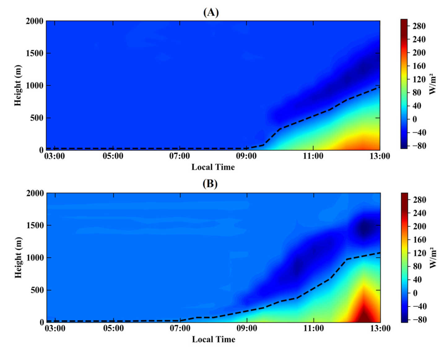
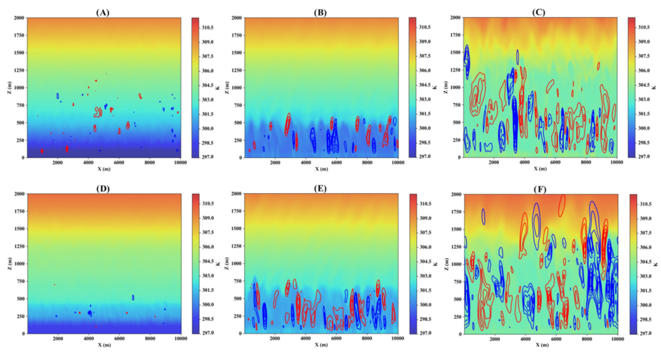
3.1. Characteristics of IOP 1 and IOP 2

The temporal evolution of the vertical profiles of the horizontally averaged sensible heat flux ( w θ ¯ ) simulated by the PALM model is presented in Figure 3 (converted from K m s−1 to W m−2, multiplied by ρ   c p ) for the rainy (IOP 1) (Figure 3A) and dry (IOP 2) periods (Figure 3B) of 2014. It is a night–daytime transition phase; thus, it is noted that during IOP 1, the profiles showed positive values (greater than 10 W m−2) after 09 LT from the surface to approximately 100 m. At 10 LT, the flux was around 100 W m−2 from the surface up to 500 m, and this layer was heated almost linearly between 10 and 13 LT. For IOP 1, the highest surface values between 11 and 13 LT were observed, of approximately 150 W m−2, resulting in a positive vertical concentration, with a maximum height of 950 m (at 13 LT). For the dry season (IOP 2), the positive values started around 7 LT, which is an earlier onset of positive values compared to IOP 1. This is due to less clouds during the dry season. Thus, after 09 LT, a more pronounced vertical development was observed, with higher values close to the surface (90.0 W m−2). The highest surface values for IOP 2 were 280 W m−2 between 12 and 13 LT and with positive vertical fluxes extending from the surface up to the top of the CBL (height of 1100 m). It is important to notice that the entrainment flux, which is a negative w θ ¯ near the top of the PBL that occurs during the daytime has its maximum after 11 LT (typically −60.0 W m−2) and above 1000 m for all IOPs.
The PBL heights obtained by PALM, between 02 to 13 LT, together with the in situ radiosonde measurements and the ceilometer estimates for the representative days of IOPs 1 and 2 are shown in Figure 4. The vertical lines represent sunrise (continuous line) and the erosion of the NBL (dashed line).
During the NBL period for the representative day of IOP 1 (Figure 4A), it was observed that the NBL was well established (between 02 and 06 LT) so that the height obtained by PALM showed a typical height around 300 m. However, some oscillations in the height of the NBL (ranging from 270 and 450 m) between 04 and 06 LT were observed. The results found by the simulation were similar to those obtained by the ceilometer during the same time interval, with an overestimation of ~50 m. For a typical day of IOP 2 (Figure 4B), during this interval, the height of the NBL was more stable at approximately 250 m. It was also observed that in the first hours of simulation (between 02 and 04 LT), the PALM model outputs underestimated (~100 m) the results found in relation to the RS and the ceilometer, and after this interval, the simulation was in agreement with the observed data. The results found for the heights of the NBL on the typical days of IOPs 1 and 2 are in agreement with the average of these IOPs, which were observed by Carneiro and Fisch [18] for the same region, verifying higher and lower fluctuations in the height of the NBL for IOPs 1 and 2, respectively. In addition, these results are similar to those reported by Neves and Fisch [26] for another site in southwestern Amazonia.
The period of NBL erosion was different between the IOPs. For IOP 1, NBL erosion occurred slowly, starting after sunrise (06 LT), and until 08 LT, the NBL extended up to 500 m. After this time, an increase in the PBL height began to be observed, which resulted in complete NBL erosion at 09 LT. The time interval required for the total erosion of the NBL (3 h) may be associated with the stronger nocturnal thermal inversion and the lower surface heating, which only occurred until 09 LT (see Figure 3A). The erosion phase of the NBL was reasonably well represented by the PALM simulation, although PALM showed greater heights related to the ceilometer (typically ~130 m). However, when compared to the RS of 08 LT, PALM showed similar heights.
The average integrated heat fluxes (described in Equations (8)–(10)) in the layer were calculated during the erosion phase of the NBL (Table 1). The average kinematic heat fluxes between sunrise (06 LT) and total erosion (09 LT) were 140.2 m K from the surface ( w θ ¯ s × Δ t ) and 119.8 m K from the top of the boundary layer ( w θ ¯ b × Δ t ) due to the entrainment for the IOP 1 representative day. Meanwhile, the heating within the entire layer ( i = 0 h Δ θ Δ z i ) was 374.4 m K, which resulted in an integrated residue of 114.4 m K (30% of the total heat). This result indicates that an additional amount of energy was used in the system, which could come from the energy released from biomass. In the present case under analysis (3 March 2014), it was also possible to include the entrainment flux contribution (119.8 m K), but that was not enough.
For the representative day of IOP 2, it was observed that the erosion of NBL was 1 h faster for this IOP in relation to IOP 1, according to Figure 4B. In IOP 2, there was an earlier initiation of surface heating, which was also more intense (see Figure 3B). During the erosion phase, it was verified that PALM results showed a satisfactory simulation in relation to the in situ measurements (RS) at 08 LT and the ceilometer, which presented a small underestimation (~15 m). The PBL heights observed in this study agree with those verified by Carneiro et al. [23] for the central Amazon’s dry season.
For IOP 2, the average kinematic heat fluxes between 06 and 08 LT were higher, especially the contribution of surface fluxes, which registered an average of 282.1 m K, while the fluxes from the top were 112.0 m K. Consequently, the total heating within the layer ( i = 0 h Δ θ Δ z i ) was 418.6 m K. There was an integrated residue of 24.5 m K (6% of the total heat).
After the erosion of the NBL, the development of the CBL begins to intensify in this period for IOP 1. This development occurred slowly, until the maximum simulation height of approximately 1200 m was observed, showing similarity with the 1150 m ceilometer height. For IOP 2, it was found that after NBL erosion, faster development of the CBL was observed, with a maximum height of 1500 m verified in PALM, demonstrating the efficiency of the model since the ceilometer showed a height of 1550 m.
Figure 5 shows the vertical profile (xz) of the potential temperature overlapped by the vertical wind speed component at 04 LT (Figure 5A,D), 08 LT (Figure 5B,E), and 10 LT (Figure 5C,F).
It was observed that for IOP 1 (Figure 5A,C and Figure 6B), the potential temperature showed a cooler atmosphere at the surface (~297 K) at 04 LT as well as weak vertical movements with intensities below 1.0 m s−1. At 08 LT, there was heating of the lower layers of the atmosphere of around 3.0 K; however, the vertical movements that occurred still had low intensity. Therefore, the vertical development of the PBL was not significant, confirming the fact that the complete erosion of the NBL had not occurred. At 10 LT, when the NBL was completely eroded, convective movements reached an average level of 1100 m, with a temperature of around 304.5 K from the base to this height, and with more intense magnitudes of the upward (3.0 m s−1) and downward (−2.5 m s−1) movements.
For IOP 2 (Figure 5D–F) at 04 LT, as also observed in IOP 1, the atmosphere was stable with thermal stratification and a potential temperature of ~297.0 K; however, vertical movements practically did not occur. At 08 LT, there was greater heating (~5.0 K) at the surface up to the height of 750 m, and due to the fact that the NBL had been completely eroded at this time, and due to the greater conversion of net radiation to sensible heat flux, an increase in convection and vertical movements was observed, which intensified both upward (with values above 1.5 m s−1) and downward (1.0 m s−1), and which resulted in the largest development of the CBL observed in this study (see Figure 4B). Thus, when analyzing the time of 10 LT, a greater warming of the atmosphere (~305.0 K) of the surface was noted up to approximately 1500 m, with this IOP presenting vertical movements with greater intensity (upward and downward movements of ~3.5 m s−1), which resulted in a well-established PBL at this time.

3.2. Modifications Due to the ENSO Event (Characteristics of IOP 3 and IOP 4)

As already mentioned, the year 2015 was an ENSO event, which caused a lot of change, especially during the second part of the year (dry season). The simulated kinematic fluxes ( w θ ¯ ) are shown in Figure 6. The IOP 3 rainy season’s characteristics (Figure 6A) showed behavior similar to IOP 1, with the occurrence of positive profiles (10.0 W m−2) after 09 LT and maximum values at the surface between 11 and 13 LT of approximately 135.0 W m−2, with a maximum height of positive fluxes of 850 m (at 13 LT).
IOP 4 (Figure 6B) showed positive values just after 07 LT and with higher values close to the surface after 09 LT. However, the higher values observed in this IOP were more intense than the same period for 2014, being in the range between 10 and 13 LT of approximately 280.0 W m−2, and with a height of 1500 m (top of CBL). This resulted in greater conversion of net radiation into sensible heat fluxes, which means that more energy was available during the 2015 dry season compared to 2014, a common feature in years with ENSO events [52]. For 2015, the entrainment zone (negative maximum flux) was −80.0 W m−2 for IOP 3 (lasting from 11 up to 13 LT) and −30.0 W m−2 for IOP 4 (between 10 and 13 LT).
The NBL heights (between 02 and 06 LT) for the representative day of IOP 3 (Figure 7A) presented heights similar to IOP 1 but with higher variability. The PALM simulation recorded heights ranging from 300 m to 475 m, overestimating the ceilometer values (~130 m). It should also be noted that the heights observed by the ceilometer also showed fluctuations ranging from 200 to 350 m. For IOP 4 (Figure 7B), PALM showed constant NBL heights of around 220 m, similar to that observed during IOP 2. During this interval (between 02 to 06 LT), the PALM results agreed with the data observed by the RS and ceilometer but with a slight underestimation (~30 m).
The NBL erosion for the rainy (IOP 3) and dry (IOP 4) periods behaved similarly to the respective periods for the typical year 2014, wherein through PALM in the IOP 3 after sunrise (06 LT), a slight increase in the height of the layer was observed, around 50.0 m h−1, between 06 and 08 LT, with complete erosion of the NBL after 09 LT. At the beginning of this phase, PALM overestimated the results found using the ceilometer (~100 m) and showed a small overestimation in relation to the RS at 08 LT (~50 m). As it was already observed for IOP 1, IOP 3′s kinematic heat medium fluxes were not sufficient to fully heat the layer (Table 2), in which the flux w θ ¯ s × Δ t was 145.4 K m, while w θ ¯ b × Δ t was 127.3 m K. A heat value of 386.2 m K was estimated as being necessary to erode the layer ( i = 0 h Δ θ Δ z i ). Thus, for this IOP, the difference between fluxes also represented ~30% of the total heating (113.5 m K), as was found for IOP 1.
At IOP 4, PALM outputs satisfactorily represented the period of the NBL erosion, in which immediately after 06 LT, there was an increase in the heights of the layer of ~150.0 m h−1 until 08 LT when the NBL was completely eroded. PALM’s heights were shown to agree with the observations made by the ceilometer and the RS (underestimating by ~15 m). During this IOP, it was possible to observe the highest average kinematic heat fluxes at the surface (292.5 m K) and at the top (146.5 m K), and the heating within the layer ( i = 0 h Δ θ Δ z i ) was 350.8 m K. Therefore, for this IOP, the released fluxes were higher than the layer’s heating, showing a difference of −88.2 m K (25% above the heating of the layer). Corroborating with what was previously demonstrated, the greater amount of energy released influenced the erosion time of the NBL and consequently the formation of an earlier CBL.
The development of the CBL for IOPs 3 and 4 reinforced that this phase is directly impacted by the time required for NBL erosion. It was verified that for IOP 3, the development occurred slowly, similar to that seen in IOP 1, with the maximum height of the CBL observed by PALM being 1250 m, while the ceilometer registered a height of 1175 m. IOP 4 showed the greatest development of the CBL throughout the study in response to increased warming of the atmosphere, leading to a greater height of CBL (1600 m).
Through a vertical plane, with thermal (Tp) and mechanical (w) information, the vertical movements during IOP 3 (Figure 8A–C) present patterns similar to those observed in IOP 1. This showed little intensity (~1.0 m s−1) at 04 and 08 LT, and with a cooler atmosphere at the surface, ~297 K at 04 LT, with an increase of 2.5 K at 08 LT. In contrast, the 10 LT warming of the atmosphere at the surface (~303.5 K) was observed, as well as more intense convective movement (~2.5 m s−1) reaching a height of ~1000 m. These results denote a lower vertical development of the CBL in response to the erosion time of the NBL.
In IOP 4 (Figure 8D–F) at 04 LT, there was a potential temperature of ~297 K, and similar to IOP 2, there were no vertical movements, indicating a very stable atmosphere. In this IOP at 08 LT, there was a formation of more intense vertical movements (~2.5 m s−1) and greater heating (~6 K) of the surface up to the layer of ~700 m. The higher estimated intensity is related to the greater conversion of net radiation to the surface in sensible heat, which was verified in this IOP. Meanwhile, at 10 LT, greater warming (~307.5 K) of the surface was observed up to approximately 1750 m, as well as more intense vertical movements (ascending and descending movements of ~3.5 m s−1).

4. Conclusions

This study showed that the PALM model presented satisfactory results in relation to the observational data for the NBL erosion phase in a region of the central Amazon. For dry IOPs (2 and 4), the heating surface observed was more pronounced after sunrise, generating more intense convection and faster erosion of the NBL, about 2 h. Meanwhile, the rainy season IOPs (1 and 3) exhibited weaker surface heating and less intense convection, which resulted in a slower erosion of the NBL, about 3 h. The time required for NBL erosion influenced the development of the CBL: a greater vertical development was observed during the dry IOPs and a greater final height, from 1500 m (IOP 2) and 1600 m (IOP 4), whereas in rainy IOPs, the maximum height was approximately 1200 m (IOPs 1 and 3).
The analyses of the kinematic heat flux in the heating of the layer during erosion were provided from the sensible heat fluxes released by the surface and the entrainment at the top of the PBL and showed that in the case of IOPs 1 and 3, the energy released was not enough to fully heat the layer, requiring more than 30% additional energy. On the other hand, IOPs 2 and 4 showed different patterns, since in IOP 2, the released energy also did not close the balance and needed approximately 6% additional energy. However, IOP 4, which was under the influence of the ENSO event, showed that the released fluxes were sufficient to fully heat the layer.
These results demonstrate that during the dry season (IOP 2 and 4), the larger heating of the layer results in faster erosion of the NBL, with more intense vertical movements and, consequently, cause a more accentuated development of the CBL. It is noteworthy that on the representative day of IOP 4, there was greater intensity of these results in response to the ENSO event.
Additionally, some recent experimental studies done by [53,54] in Antarctica and Russia showed clearly the presence of waves that looked like Kelvin–Helmholtz billows in the elevating inversion layer rising above the convective layer. So, this is an open question whether these waves can have an influence on the erosion of the NBL for Amazonia, which has a weak, stable boundary layer compared to the Antarctica and Russia regions. Thus, the development of algorithms to take into account the presence of this phenomenon could help to improve the modeling results.

Author Contributions

All authors contributed to the research and to the collaboration of this manuscript. R.C., G.F. and R.S. participated in the data collection campaigns of the GoAmazon project; R.C. and G.F. designed the numerical experiments; R.C. performed the simulations as part of his PhD and processed and analyzed the data, assisted by G.F. and prepared the first draft of this paper and the write-up of the manuscript; and G.F., T.N., C.B., C.S. and R.S. analyzed the data, provided guidelines for the write-up of the manuscript, and contributed to its editing and finalization. All authors have read and agreed to the published version of the manuscript.

Funding

This study was financed in part by the Coordenação de Aperfeiçoamento de Pessoal de Nível Superior-Brazil (CAPES)-Finance Code 001 and has been supported by the National Council for Scientific and Technological Development (grant No. 140726/2017-9).

Data Availability Statement

The data sets used in this publication are available at the ARM Climate Research Facility database for the GoAmazon 2014/5 experiment (https://www.arm.gov/research/campaigns/amf2014goamazon (accessed on 3 February 2021) (ARM Climate Research Facility, 2019)).

Acknowledgments

The authors thank the National Institute of Space Research (INPE), the National Institute of Amazonian Research (INPA), and Amazonas State University (UEA) for institutional support. Rayonil Carneiro acknowledges the Brazilian National Council for Scientific and Technological Development (CNPq) and Coordination for the Improvement of Higher Education Personnel (CAPES) for the graduate fellowship. Gilberto Fisch and Carlos Santos also acknowledge CNPq for providing them with research productivity grants (processes Nos. 307048/2018-7 and 304493/2019-8, respectively). The authors thank the GoAmazon project group for providing the data available for this study.

Conflicts of Interest

The authors declare that they have no conflict of interest. The founding sponsors had no role in the design of the study; in the collection, analyses, or interpretation of data; in the writing of the manuscript; or in the decision to publish the results.

References

  1. Marengo, J.A.; Espinoza, J.C. Extreme seasonal droughts and floods in Amazonia: Causes, trends and impacts. Int. J. Climatol. 2016, 36, 1033–1050. [Google Scholar] [CrossRef]
  2. Martin, S.T.; Artaxo, P.; Machado, L.A.T.; Manzi, A.O.; Souza, R.A.F.; Schumacher, C.; Wang, J.; Andreae, M.O.; Barbosa, H.M.J.; Fan, J.; et al. Introduction: Observations and modeling of the Green Ocean Amazon (GoAmazon2014/5). Atmos. Chem. Phys. 2016, 16, 4785–4797. [Google Scholar] [CrossRef] [Green Version]
  3. Marengo, J.A.; Fisch, G.F.; Alves, L.M.; Sousa, N.V.; Fu, R.; Zhuang, Y. Meteorological context of the onset and end of the rainy season in Central Amazonia during the GoAmazon2014/5. Atmos. Chem. Phys. 2017, 17, 7671–7681. [Google Scholar] [CrossRef] [Green Version]
  4. Machado, L.A.; Calheiros, A.J.; Biscaro, T.; Giangrande, S.; Dias, M.A.; Cecchini, M.A.; Albrecht, R.; Andreae, M.O.; Araujo, W.F.; Artaxo, P.; et al. Overview: Precipitation characteristics and sensitivities to environmental conditions during GoAmazon2014/5 and ACRIDICON-CHUVA. Atmos. Chem. Phys. 2018, 18, 6461–6482. [Google Scholar] [CrossRef] [Green Version]
  5. Stull, R.B. An. Introduction to Boundary Layer Meteorology, 1st ed.; Springer Science & Business Media: Dodrecht, The Netherlands, 1988; p. 670. [Google Scholar]
  6. Steeneveld, G.J. Current challenges in understanding and forecasting stable boundary layers over land and ice. Front. Environ. Sci. 2014, 2, 1–6. [Google Scholar] [CrossRef] [Green Version]
  7. Mahrt, L. Stably stratified atmospheric boundary layers. Annu. Rev. Fluid Mech. 2014, 46, 23–45. [Google Scholar] [CrossRef] [Green Version]
  8. Mahrt, L. Stably stratified flow in a shallow valley. Bound. Layer Meteorol. 2017, 162, 1–20. [Google Scholar] [CrossRef]
  9. Sun, J.; Mahrt, L.; Banta, R.; Pichugina, Y.L. Turbulence regimes and turbulence intermittency in the stable boundary layer during CASES99. J. Atmos. Sci. 2012, 69, 338–351. [Google Scholar] [CrossRef] [Green Version]
  10. Pfister, L.; Sayde, C.; Selker, J.; Mahrt, L.; Thomas, C.K. Classifying the nocturnal boundary layer into temperature and flow regimes. Q. J. R. Meteorol. Soc. 2019, 145, 1515–1534. [Google Scholar] [CrossRef]
  11. Sun, J.; Lenschow, D.H.; LeMone, M.A.; Mahrt, L. The role of large-coherent eddy transport in the atmospheric surface layer based on CASES-99 observations. Bound. Layer Meteorol. 2016, 160, 83–111. [Google Scholar] [CrossRef]
  12. Zhang, W.; Guo, J.; Miao, Y.; Liu, H.; Zhang, Y.; Li, Z.; Zhai, P. Planetary boundary layer height from CALIOP compared to radiosonde over China. Atmos. Chem. Phys. 2016, 16, 9951–9963. [Google Scholar] [CrossRef] [Green Version]
  13. Luo, T.; Yuan, R.; Wang, Z. Lidar-based remote sensing of atmospheric boundary layer height over land and ocean. Atmos. Meas. Tech. 2014, 7, 173–182. [Google Scholar] [CrossRef] [Green Version]
  14. Wang, X.Y.; Wang, K.C. Estimation of atmospheric mixing layer height from radiosonde data. Atmos. Meas. Tech. 2014, 7, 1701–1709. [Google Scholar] [CrossRef] [Green Version]
  15. Wang, D.; Stachlewska, I.S.; Song, X.; Heese, B.; Nemuc, A. Variability of the Boundary Layer Over an Urban Continental Site Based on 10 Years of Active Remote Sensing Observations in Warsaw. Remote. Sens. 2020, 12, 340. [Google Scholar] [CrossRef] [Green Version]
  16. Acevedo, O.C.; Maroneze, R.; Costa, F.D.; Puhales, F.S.; Degrazia, G.A.; Martins, L.G.N.; Oliveira, P.E.S.; Mortarini, L. The nocturnal boundary layer transition from weakly to very stable. Part I Obs. Q. J. R. Meteorol. Soc. 2019, 145, 3577–3592. [Google Scholar] [CrossRef]
  17. Uzan, L.; Egert, S.; Khain, P.; Levi, Y.; Vadislavsky, E.; Alpert, P. Ceilometers as planetary boundary layer height detectors and a corrective tool for COSMO and IFS models. Atmos. Chem. Phys. 2020, 20, 12177–12192. [Google Scholar] [CrossRef]
  18. Carneiro, R.G.; Fisch, G. Observational analysis of the daily cycle of the planetary boundary layer in the central Amazon during a non-El Niño year and El Niño year (GoAmazon project 2014/5). Atmos. Chem. Phys. 2020, 20, 5547–5558. [Google Scholar] [CrossRef]
  19. Marley, H.G.; Dirks, K.N.; McKendry, I.; Weissert, L.F.; Salmond, J.A. A Ceilometer-Derived Climatology of the Convective Boundary Layer Over a Southern Hemisphere Subtropical City. Bound. Layer Meteorol. 2020. [Google Scholar] [CrossRef]
  20. Neves, T.; Fisch, G.; Raasch, S. Local convection and turbulence in the Amazonia using large eddy simulation model. Atmosphere 2018, 9, 3990. [Google Scholar] [CrossRef] [Green Version]
  21. Yee, L.D.; Isaacman-VanWertz, G.; Wernis, R.A.; Meng, M.; Rivera, V.; Kreisberg, N.M.; Hering, S.V.; Bering, M.S.; Glasius, M.; Upshur, M.A.; et al. Observations of sesquiterpenes and their oxidation products in central Amazonia during the wet and dry seasons. Atmos. Chem. Phys. 2018, 18, 10433–10457. [Google Scholar] [CrossRef] [Green Version]
  22. Wang, W.; Gong, W.; Mao, F.; Pan, Z. An Improved Iterative Fitting Method to Estimate Nocturnal Residual Layer Height. Atmosphere 2016, 7, 106. [Google Scholar] [CrossRef] [Green Version]
  23. Carneiro, R.G.; Fisch, G.; Borges, C.K.; Henkes, A. Erosion of the nocturnal boundary layer in the central Amazon during the dry season. Acta Amaz. 2020, 50, 80–89. [Google Scholar] [CrossRef]
  24. Santos, L.R.; Fisch, G. Intercomparison between four methods of estimating the height of the convective boundary layer during the RACCI-LBA (2002) experiment in Rondônia-Amazonia. Rev. Bras. Meteorol. 2007, 22, 322–328. [Google Scholar] [CrossRef] [Green Version]
  25. Seidel, D.J.; Ao, C.O.; Li, K. Estimating climatological planetary boundary layer heights from radiosonde observations: Comparison of methods and uncertainty analysis. J. Geophys. Res. Atmos. 2010, 115, 1–15. [Google Scholar] [CrossRef] [Green Version]
  26. Neves, T.T.A.; Fisch, G. Nocturnal boundary layer over an Amazonian pasture area. Rev. Bras. Meteorol. 2011, 24, 619–628. [Google Scholar] [CrossRef] [Green Version]
  27. Shukla, K.K.; Phanikumar, D.V.; Newsom, R.K.; Kumar, K.N.; Ratnam, M.V.; Naja, M.; Singh, N. Estimation of the mixing layer height over a high altitude site in Central Himalayan region by using Doppler Lidar. J. Atmos. Sol. Terr. Phys. 2014, 109, 48–53. [Google Scholar] [CrossRef]
  28. Wiegner, M.; Madonna, F.; Binietoglou, I.; Forkel, R.; Gasteiger, J.; Geiß, A.; Pappalardo, G.; Schäfer, K.; Thomas, W. What is the benefit of ceilometers for aerosol remote sensing? An answer from EARLINET. Atmos. Meas. Tech. 2014, 7, 1979–1997. [Google Scholar] [CrossRef] [Green Version]
  29. Morris, V. Ceilometer Instrument Handbook; Pacific Northwest National Laboratory: Richland, WA, USA, 2016. [Google Scholar]
  30. Geiß, A.; Wiegner, M.; Bonn, B.; Schäfer, K.; Forkel, R.; von Schneidemesser, E.; Münkel, C.; Chan, K.L.; Nothard, R. Mixing layer height as an indicator for urban air quality? Atmos. Meas. Tech. 2017, 10, 2969–2988. [Google Scholar] [CrossRef] [Green Version]
  31. Burba, G. Eddy Covariance Method for Scientific, Industrial, Agricultural and Regulatory Applications: A Field Book on Measuring Ecosystem Gas Exchange and Areal Emission Rates; Li-Cor Biosciences: Lincoln, ME, USA, 2013. [Google Scholar] [CrossRef]
  32. Sullivan, P.P.; Weil, J.C.; Patton, E.G.; Jonker, H.J.J.; Mironov, D.V. Turbulent winds and temperature fronts in Large-Eddy Simulations of the stable atmospheric boundary layer. J. Atmos. Sci. 2016, 73, 1815–1838. [Google Scholar] [CrossRef] [Green Version]
  33. Schwenkel, J.; Maronga, B. Towards a better representation of fog microphysics in Large-Eddy Simulations based on an embedded lagrangian cloud model. Atmosphere 2020, 11, 466. [Google Scholar] [CrossRef]
  34. El Guernaoui, O.; Reuder, J.; Esau, I.; Wolf, T.; Maronga, B. Scaling the Decay of Turbulence Kinetic Energy in the Free-Convective Boundary Layer. Bound. Layer Meteorol. 2019, 173, 79–97. [Google Scholar] [CrossRef] [Green Version]
  35. Raasch, S.; Schröter, M. PALM-A large-eddy simulation model performing on massively parallel computers. Meteorol. Z. 2001, 10, 363–372. [Google Scholar] [CrossRef]
  36. Maronga, B.; Gryschka, M.; Heinze, R.; Hoffmann, F.; Kanani-Sühring, F.; Keck, M.; Ketelsen, K.; Letzel, M.O.; Sühring, M.; Raasch, S. The Parallelized Large-Eddy Simulation Model (PALM) version 4.0 for atmospheric and oceanic flows: Model formulation, recent developments, and future perspectives. Geosci. Model. Dev. 2015, 8, 2515–2551. [Google Scholar] [CrossRef] [Green Version]
  37. Maronga, B.; Banzhaf, S.; Burmeister, C.; Esch, T.; Forkel, R.; Fröhlich, D.; Fuka, V.; Gehrke, K.F.; Geletič, J.; Giersch, S.; et al. Overview of the PALM model system 6.0. Geoscientific Model. Development 2020, 13, 1335–1372. [Google Scholar] [CrossRef]
  38. Raasch, S.; Franke, T. Structure and formation of dust- devil-like vortices in the atmospheric boundary layer: A high resolution numerical study. J. Geophys. Res. 2011, 116, D16120. [Google Scholar] [CrossRef]
  39. Maronga, B.; Raasch, S. Large-eddy simulations of surface heterogeneity effects on the convective boundary layer during the LITFASS-2003 experiment. Bound. Layer Meteorol. 2013, 146, 17–44. [Google Scholar] [CrossRef] [Green Version]
  40. Maronga, B.; Hartogensis, O.K.; Raasch, S.; Beyrich, F. The effect of surface heterogeneity on the structure parameters of temperature and specific humidity: A large-eddy simulation case study for the LITFASS-2003 experiment. Bound. Layer Meteorol. 2014, 153, 441–470. [Google Scholar] [CrossRef] [Green Version]
  41. Kanani-Sühring, F.; Raasch, S. Enhanced scalar concentrations and fluxes in the lee of forest patches: A large-eddy simulation study. Bound. Layer Meteorol. 2017, 164, 1–17. [Google Scholar] [CrossRef]
  42. Deardorff, J.W. Stratocumulus-capped mixed layers derived from a three-dimensional model. Bound. Layer Meteorol. 1980, 18, 495–527. [Google Scholar] [CrossRef]
  43. Moeng, C.H.; Wyngaard, J.C. Spectral analysis of large-eddy simulations of the convective boundary layer. J. Atmos. Sci. 1988, 45, 3573–3587. [Google Scholar] [CrossRef] [Green Version]
  44. Saiki, E.M.; Moeng, C.H.; Sullivan, P.P. Large-eddy simulation of the stably stratified planetary boundary layer. Bound. Layer Meteorol. 2000, 95, 1–30. [Google Scholar] [CrossRef] [Green Version]
  45. Moeng, C.-H. A large-eddy-simulation model for the study of planetary boundary-layer turbulence. J. Atmos. Sci. 1984, 41, 2052–2062. [Google Scholar] [CrossRef]
  46. Mason, P.J. Large-eddy simulation: A critical review of the technique. Q. J. R. Meteorol. Soc. 1994, 120, 1–26. [Google Scholar] [CrossRef]
  47. Shaw, R.H.; Schumann, U. Large-eddy simulation of turbulent flow above and within a forest. Bound. Layer Meteorol. 1992, 61, 47–64. [Google Scholar] [CrossRef] [Green Version]
  48. Watanabe, T. Large-eddy simulation of coherent turbulence structures associated with scalar ramps over plant canopies. Bound. Layer Meteorol. 2004, 112, 207–341. [Google Scholar] [CrossRef]
  49. Wicker, L.J.; Skamarock, W.C. Time-splitting methods for elastic models using forward time schemes. Mon. Weather. Rev. 2002, 130, 2088–2097. [Google Scholar] [CrossRef]
  50. Williamson, J.H. Low-storage Runge–Kutta schemes. J. Comput. Phys. 1980, 35, 48–56. [Google Scholar] [CrossRef]
  51. Vernekar, K.G.; Mohan, B.; Saxena, S.; Patil, M.N. Characteristics of the atmospheric boundary layer over a tropical station as evidenced by tethered ballon observations. J. Appl. Meteorol. 1993, 32, 1426–1432. [Google Scholar] [CrossRef]
  52. Macedo, A.S.; Fisch, G. Temporal variability of solar radiation during the GOAmazon 2014/15 experiment. Rev. Bras. Meteorol. 2018, 33, 353–365. [Google Scholar] [CrossRef]
  53. Petenko, I.; Argentini, S.; Casasanta, G.; Kallistratova, M.; Sozzi, R.; Viola, A. Wavelike structures in the turbulent layer during the morning development of convection at Dome C., Antarctica. Bound. Layer Meteorol. 2016, 161, 289–307. [Google Scholar] [CrossRef] [Green Version]
  54. Kallistratova, M.A.; Petenko, I.V.; Kouznetsov, R.D.; Kuznetsov, D.D.; Lyulyukin, V.S.; Perepelkin, V.G. Kelvin-Helmholtz billows in rising morning inversions. IOP Conf. Ser. Earth Environ. Sci. 2019, 231, 012025. [Google Scholar] [CrossRef]
Figure 1. Geographic location of the Municipality of Manacapuru, Amazonas, and the T3 study area.
Atmosphere 12 00240 g001
Figure 2. Schematic diagram of the potential temperature profiles at 06 LT (full line) and NBL erosion time (dashed line). The gray area represents the thermal heating of the layer between the two profiles necessary to erode the NBL. (Source: Carneiro et al. [23]).
Atmosphere 12 00240 g002
Figure 3. Time series of the vertical profiles of the horizontally averaged sensible heat flux ( w θ ¯ ) simulated by the PALM model over the GoAmazon site for (A) IOP 1 and (B) IOP 2. The dashed line represents the height where the flux is null ( w θ ¯ = 0).
Atmosphere 12 00240 g003
Figure 4. Heights of the PBL over the GoAmazon site for (A) IOP 1 and (B) IOP 2. The vertical lines mark sunrise (continuous line) and the erosion of the NBL (dashed line).
Atmosphere 12 00240 g004
Figure 5. Plane xz (y = 5.0 km) of potential temperature (K) and vertical wind contours (m s−1), colors (line) representing upward (blue) and downward (red) movements, at different times of the day for (AC) IOP 1 and (DF) IOP 2, where the local time is (A,D) 04 LT, (B,E) 08 LT, and (C,F) 10 LT.
Atmosphere 12 00240 g005
Figure 6. Time series of the vertical profiles of the horizontally averaged sensible heat flux ( w θ ¯ ) simulated by the PALM model over the GoAmazon site for (A) IOP 3 and (B) IOP 4. The dashed line represents the height where the flux is zero ( w θ ¯ = 0).
Atmosphere 12 00240 g006
Figure 7. Heights of the PBL (m) over the GoAmazon site for (A) IOP 3 and (B) IOP 4. The vertical lines mark sunrise (continuous line) and the erosion of the NBL (dashed line).
Atmosphere 12 00240 g007
Figure 8. Plane xz (y = 5.0 km) of potential temperature (K) and vertical wind contours (m s−1), colors (line) representing upward (blue) and downward (red) movements, at different times of the day for (AC) IOP 3 and (DF) IOP 4, where the local time is (A,D) 04 LT, (B,E) 08 LT, and (C,F) 10 LT.
Atmosphere 12 00240 g008
Table 1. Integrated total heat flux for the NBL erosion period on the surface ( w θ ¯ s × Δ t ), top layer flux ( w θ ¯ b × Δ t ), and layer heating ( i = 0 h Δ θ Δ z i ) during IOP 1 and IOP 2.
NBL Erosion: IOP 1
Period
(Hour)
w θ ¯ s × Δ t (m K) w θ ¯ b × Δ t (m K) i = 0 h Δ θ Δ z i (m K)
06–09140.2119.8374.4
NBL Erosion: IOP 2
Period
(Hour)
w θ ¯ s × Δ t (m K) w θ ¯ b × Δ t (m K) i = 0 h Δ θ Δ z i (m K)
06–08282.1112.0418.6
Table 2. Integrated total heat flux for the NBL erosion period at the surface ( w θ ¯ s × Δ t ), top layer flux ( w θ ¯ b * Δ t ), and layer heating ( i = 0 h Δ θ Δ z i ) during IOP 3 and IOP 4.
NBL Erosion: IOP 3
Period
(Hour)
w θ ¯ s × Δ t (m K) w θ ¯ b × Δ t (m K) i = 0 h Δ θ Δ z i (m K)
06–09145.4127.3386.2
NBL Erosion: IOP 4
Period
(Hour)
w θ ¯ s × Δ t (m K) w θ ¯ b × Δ t (m K) i = 0 h Δ θ Δ z i (m K)
06–08292.5146.5350.8
Publisher’s Note: MDPI stays neutral with regard to jurisdictional claims in published maps and institutional affiliations.

