Article

Reanalysis Product-Based Nonstationary Frequency Analysis for Estimating Extreme Design Rainfall

1
Office 2.17, Queens Bulding, Water and Environment Research Group, Department of Civil Engineering, University of Bristol, Bristol BS8 1TL, UK
2
Department of Civil Engineering, ERI, Gyeongsang National University, Jinju 501, Korea
*
Authors to whom correspondence should be addressed.
Atmosphere 2021, 12(2), 191; https://doi.org/10.3390/atmos12020191
Submission received: 14 January 2021 / Revised: 25 January 2021 / Accepted: 27 January 2021 / Published: 31 January 2021

Abstract

:
Nonstationarity is one major issue in hydrological models, especially in design rainfall analysis. Design rainfalls are typically estimated by annual maximum rainfalls (AMRs) of observations below 50 years in many parts of the world, including South Korea. However, due to the lack of data, the time-dependent nature may not be sufficiently identified by this classic approach. Here, this study aims to explore design rainfall with nonstationary condition using century-long reanalysis products that help one to go back to the early 20th century. Despite its useful representation of the past climate, the reanalysis products via observational data assimilation schemes and models have never been tested in representing the nonstationary behavior in extreme rainfall events. We used daily precipitations of two century-long reanalysis datasets as the ERA-20c by the European Centre for Medium-Range Weather Forecasts (ECMWF) and the 20th century reanalysis (20CR) by the National Oceanic and Atmospheric Administration (NOAA). The AMRs from 1900 to 2010 were derived from the grids over South Korea. The systematic errors were downgraded through quantile delta mapping (QDM), as well as conventional stationary quantile mapping (SQM). The evaluation result of the bias-corrected AMRs indicated the significant reduction of the errors. Furthermore, the AMRs present obvious increasing trends from 1900 to 2010. With the bias-corrected values, we carried out nonstationary frequency analysis based on the time-varying location parameters of generalized extreme value (GEV) distribution. Design rainfalls with certain return periods were estimated based on the expected number of exceedance (ENE) interpretation. Although there is a significant range of uncertainty, the design quantiles by the median parameters showed the significant relative difference, from −30.8% to 42.8% for QDM, compared with the quantiles by the multi-decadal observations. Even though the AMRs from the reanalysis products are challenged by various errors such as quantile mapping (QM) and systematic errors, the results from the current study imply that the proposed scheme with employing the reanalysis product might be beneficial to predict the future evolution of extreme precipitation and to estimate the design rainfall accordingly.

1. Introduction

Design rainfall plays an essential role in planning a water-related infrastructure and it has been commonly estimated from the precipitation intensity–duration–frequency (IDF) relationship based on the historical records with the stationary assumption [1,2]. However, recent research has indicated that many regions over the world have experienced the pattern change of climatic extremes, especially for heavy rainfall [3,4]. Recalling that a water-related project is designed under stationary condition in practice, the temporal change of extreme rainfalls, so-called ‘nonstationarity’, may significantly affect the safety of the infrastructure. In other words, an increasing trend in heavy rainfall can underestimate the estimated future risk when an obvious trend exists in a target region. Note that the hypothesis of a non-stationary model can be altered by the presence of outliers with assuming parameters as random variables, while preserving the hypothesis of a stationary process [5].
The other major issue in rainfall frequency analysis is the lack of the gauge data resulting in significant errors in hydrological modellings. In a block maxima (BM) approach typically used in practical application, one generally collects annual maximum rainfalls (AMRs) from historical records to derive IDF relationships. However, in many regions including South Korea, the long-term meteorological record for a given catchment is largely limited to create the reliable IDF relationships. For instance, South Korea, with an area of approximately 100,032 km 2 , has over hundreds of weather stations, but the number of stations with daily rainfalls over 40 years was at most a few dozen by the Korean War. Consequently, the rainfall quantiles are derived from less than 40-year data and necessarily contain significant uncertainties, which are associated with the sampling errors [6,7,8,9,10].
Furthermore, the use of external source is also critical to respect the ergodicity [11,12], since the properties of a stochastic process might be estimated only by limited observations. When the process is nonstationary, the ergodicity cannot hold and possible trends should be derived from external sources, different from observed time series.
Subsequently, the future risk in a region like South Korea can be relabily estimated by considering the nonstationary and extending the data length is critical. However, existing studies have explored individual aspects, but there have been no studies to combine two factors, nonstationarity and lack of data, at the same time. Thus, this study aims to reliably extend the data series, and then to explore the future risk change (i.e., nonstationarity) with the extended time series, which may depend on time, in South Korea.
To address the lack of data, we introduce long-term reanalysis datasets as substitutes of the observed. With their own assimilation techniques, reanalysis products have been globally provided with daily or sub-daily resolution and they have been applied in the global-, continental- and country-scale climate change analyses [13,14,15,16,17,18]. However, most reanalysis products provide the climate variables after the 1950s, and a few datasets assimilated by two representative institutes, the National Oceanic and Atmospheric Administration (NOAA) and the European Centre for Medium-Range Weather Forecasts (ECMWF), can cover the whole 20th century; the 20th century reanalysis (20CR) by the NOAA, and ERA-20c and ERA-20 cm by the ECMWF [15,18,19]. For ERA-20c and ERA-20cm by the ECMWF, they are based on the same simulation model, but ERA-20 cm does not consider observations in the assimilation process, unlike ERA-20c. For this reason, ERA-20c has a limitation in representing the actual synoptic situation [15,16,17,18]. Thus, we use two reanalysis datasets, 20CR and ERA-20c, produced by two different institutes as substitutes of the observed.
Like other model data, long-term reanalysis datasets include the systematic errors which vary with space [17,20]. Thus, the bias correction of reanalysis products, especially for regional-scale studies, should be performed before hydrologic applications. Numerous studies have suggested various bias correction methods from a delta change to a quantile mapping (QM) or multivariate scheme using a copula-based principle [17,21,22,23,24]. Each method has its pros and cons, but a QM method has been commonly used for precipitation due to its good performance [21,25,26,27]. We also improve the biases in the modelled by using a QM approach. In the BM principle, estimating IDFs are based on the AMRs of the data. Thus, the purpose of bias correction in this study is to collect the improved AMRs, and there are two main approaches for it; (1) to improve the whole rainfall distribution and derive the AMRs and (2) to directly correct the AMRs of the modelled. Compared with the former approach, the direct correction approach does not need to consider ‘drizzling effect’, which can impair the bias corrected values, and the errors in IDFs were less than that by improving whole wet-day data [2]. In this context, we collect the AMRs directly from the reanalysis products and then improve them with the QM approach.
To perform a nonstationary frequency analysis, it is essential to detect the significant long-term trends of the data. Previous studies for South Korea have documented that rainfalls have increased over time, especially during summer [28,29,30,31,32,33,34]. However, if we only focus on the ‘AMRs’, it is also true that there is no clear evidence for the trend in the AMRs of the observed [35]. Nadarajah and Choi [35] explored the trends of the AMRs for the observed in five stations over South Korea from 1961 to 2001, but there were no significant trends. For this reason, we assess the long-term trend of the AMRs for the bias-corrected from 1900 to 2010 as well as for the observed during the reference period (1974 to 2010). After detecting the significant trend, we estimate the design quantiles with the nonstationary return period.
To consider nonstationarity for rainfall or flood frequency analysis, numerous studies have commonly adopted a time-varying parameter scheme [36,37,38,39,40,41]. Conceptually, this approach assumes that a climate variable like daily rainfall has the same distribution function type, typically generalized extreme value (GEV) distribution, but the parameters are dependent on time. In this concept, a return period ( T t = 1 / ( 1 F z ( z q 0 , θ t ) ) with a certain design quantile ( z q 0 ) at time t can be easily derived from a cumulative distribution ( F z ) with the time-varying parameters ( θ t ) [42]. However, as estimating a quantile with a target period, for example 100-year, varies by time, the use of a “return period” concept can be meaningless under nonstationary condition [37,42,43].
However, as the notion of return period can still provide intuitive information to engineers, numerous studies have handled this issue and two different approaches have been proposed; the expected waiting time (EWT) approach and the expected number of exceedance (ENE) approach [42,44,45,46,47]. The former scheme, EWT, focuses on the ‘expected waiting time’ for the first occurrence exceeding the design rainfall ( z q 0 ). On the other hand, the ENE approach obtains the target value by setting the expected number of exceedances over the design life T. Both concepts should be numerically solved to estimate the design quantile with a target return period under nonstationary condition. However, conceptually, the EWT method has a drawback that this concept needs infinite (or as long as possible) future exceedance probabilities, which can cause uncertainty [42,47]. For this reason, the ENE interpretation is considered for the nonstationary analysis in this study.
As aforementioned, the primary goal of this study is to explore design rainfall with non-stationary condition using the bias-corrected reanalysis products covering from 1900 to 2010. For this purpose, this study performs a three-step approach. First, we reduce the biases in ERA-20c and 20CR, especially for the AMRs, by using a QM approach. Secondly, we evaluate long-term trends of the AMRs for the observed and the reanalysis products to detect the nonstationarity. The final step in this study is to evaluate the design rainfalls under nonstationary condition and to compare them with the results by the classic observation-based estimation. This three-step analysis is based on the mainland of South Korea, and the detailed information on the study site and data used in this study is described in Section 2. The theoretical background for the methodology is introduced in Section 3. The results and discussion are summarized in Section 4 and Section 5, respectively. Finally, the summary and conclusions are provided in Section 6.

2. Study Site and Data

2.1. Study Site and Local Gauge Data

This study is based on the mainland of South Korea, which lies between latitudes 34°–38.5° N and longitudes 126°–129.5° E, excluding all the islands including Jeju. The local gauge records are typically used for hydrologic applications, including frequency analysis. For South Korea, only dozens of weather stations can provide historical records for more than 40 years among hundreds of gauging stations. Thus, we obtained 48 in situ daily precipitation data, covering from 1974 to 2017, in the mainland of South Korea. After collecting the daily data from the Korea Meteorological Administration (http://www.kma.go.kr), we derived the annual maximum rainfalls (AMRs) for bias correction in all 48 stations. Note that, for St. 14 Andong, we ignored the AMRs from 1978 to 1982 due to the absence of records during the period. The daily AMR sequences were collected and compiled from the Korea Meteorological Administration (KMA). The coverage of the study area and the weather stations chosen in this study is shown in Figure 1, and the information for the stations is described in Table 1.

2.2. Reanalysis Products

In this study, we apply two representative century-long reanalysis products as ERA-20c by the ECMWF and 20CR by the NOAA. The ERA-20c was produced by assimilation technique using observations of surface pressure and surface marine winds only, and the product can globally cover the period from 1900 to 2010 with the spatio-temporally various resolutions [18]. On the other hand, 20CR, the first century-long reanalysis products by the NOAA, was assimilated with the ensemble Kalman filter technique using only surface pressure observations [19] and its latest version 2c could span the period from 1851 to 2014 with a spatial resolution of 1.875° × 1.9°. As the long-term climate records play an important role in the nonstationary analysis, we collect daily rainfall data from these two century-long reanalysis products in this study. More specifically, we extracted the daily precipitation records from 1900 to 2010, with the finest spatial resolution, 0.125° × 0.125° for ERA-20c and 1.875° × 1.9° for 20CR, respectively. From these daily rainfall series, this study derived the AMRs at grids in the mainland of South Korea from 1900 to 2010. The grid points over the sea were ignored in this analysis. The specific grid-scale points for ERA-20c and 20CR are shown in Figure 1. Note that only two grid points of 20CR covered the entire study region due to its low spatial resolution.
These reanalysis products are employed in a number of climatological studies [48,49,50,51]. Diro et al. [49] evaluated the spatial pattern of rainfall estimates for the reanalysis product of ERA-40 and noted that the product captures well the annual cycle over most of the country. Berntell et al. [48] investigated the strong multidecadal variability of the summer rainfall during the 20th century with reanalysis products and reported that the reanalysis product ERA-20CM shows the best representation of the multidecadal rainfall variability. Hua, et al. [51] assessed reanalysis products with quality-controlled radisonde observations and observed datasets to understand the rainfall climatology and variability over Central Equatorial Africa.

3. Methodology

3.1. Bias Correction

Although the century-long reanalysis precipitation data adopt the observed data when modeling, the modeled data still include the substantial biases. The bias correction approach should preliminarily be applied to the model values before further hydrologic applications. In the current study, we first carried out the bias correction by a quantile mapping (QM) approach, typically adopted in the bias correction studies [31,33,52,53]. Conceptually, the QM method reduces the errors by fitting a cumulative distribution of the modelled into that of the observed via a transfer function [21,53,54,55] (see Supplementary Material for detail).
For estimating the design rainfalls, BM approach using the AMRs is commonly adopted. To implement a reanalysis products-based BM approach, the bias-corrected AMRs should be collected and there are two approaches to collect them. Firstly, we can correct all wet-day precipitation data by QM methods and then, take the AMRs from the bias-corrected daily values. The other option is to directly improve the uncorrected AMRs by QM methods without considering the other rainfall data. If they are interested not only in the AMRs but also in all daily rainfalls, it would be better to apply the first option. However, as this study only focuses on exploring the non-stationary design rainfalls based on the BM, we utilize the latter option, which can reduce the error more efficiently than correcting the entire rainfall series [2]. To find out the most fitted transfer function, we applied three representative distributions, gamma, Gumbel, and GEV, for the bias correction of the AMRs, which are commonly employed in hydrologic application and extreme study [22,53,56,57]. As a QM approach is based on a one-to-one relationship, we matched 48 weather stations with the closest grid points of the ERA-20c and 20CR, and the bias-corrected values were collected at each station. Here, we assumed that the difference of spatial resolution between datasets can be ignored. One major issue in bias correction for a climate model data is how to correct the model values beyond the time range of the observation. The conventional approach of the QM algorithm was implemented with the assumption that the climate records are stationary for the whole projected period [18,28]. More specifically, the CDFs of the observed and the modeled are estimated using records for a reference period (i.e., historical period or calibration period), and the model data for the whole projected period are applied to this correction factor.
In this concept, the years from 1974 to 2010 were set as the reference period, while the whole period from 1900 to 2010 was considered as the projected period. For the stationary quantile mapping (SQM) scheme, there exist some extreme values beyond the range of the reference period, which may overestimate the bias-correction results, so an appropriate extrapolation scheme should be considered for them [2,25,33]. In the current study, we applied a constant extrapolation, which uses the correction values at the lowest and highest quantiles of the calibration range, suggested by Themeßl, Gobiet and Heinrich [25] to the events beyond the range of reference data, while the AMRs within the range were corrected by parametric approaches based on three different distributions, GEV, gamma, and Gumbel. Note that the SQM approaches with the GEV, gamma, and Gumbel were abbreviated as gevSQM and gamSQM and gumSQM, respectively.
One major problem in SQM approach is to ignore time-dependent characteristic such as a long-term trend. To handle this issue, several approaches have been tested, such as detrended quantile mapping and quantile delta approach [58,59]. Among these approaches, we applied the quantile delta mapping (QDM) method suggested by Cannon, Sobie and Murdock [31], because this approach can preserve the changes, not only in mean but also in extremes for the modelled data. In QDM, long-term trends in data are preserved by superimposing the relative change of quantiles between the reference period and the projected period, which are set to the same length. Thus, we first set the reference period to 1974–2010 as in SQM, and then divided the past projected period (1900–1973) into two periods, 1900–1936 and 1937–1973, to make the intervals equal to the reference period. Consequently, reanalysis daily precipitations were divided into three time periods with the same length (1900–1936, 1937–1973, 1974–2010) and the raw models in each time period were improved by the QDM principle [31,33] (see Supplementary Material for detail).
In this analysis, we compared the bias-corrected AMRs by QM approaches with the observations in 48 stations for the reference period (1974–2010). As the results by QDM approaches are identical to those by SQM schemes for the reference period, the QDM results were used to evaluate the performances of three different curves for the bias correction scheme.

3.2. Detecting Nonstationarity: Long-Term Trend Test

As aforementioned in the introduction section, the conventional approach for bias correction is based on the stationary condition for climate model records, but the real climate may follow the non-stationary feature in terms of century-long trend. To find out the significance of the AMR trend over South Korea, we evaluated the long-term trends of the observation and the bias corrected reanalysis data. For the trend test, a non-parametric method, the Mann–Kendall test was applied in this study. The significance of trends was evaluated by comparing the test statistic Z with the standard normal variate at the desired significance [60]. When | Z | > Z 1 α / 2   for the standard normal deviate Z 1 α / 2   with the significance level α (=0.05 in the current study), the null hypothesis is rejected and a significant trend in a time series. For the slope, the Theil–Sen approach [61,62,63,64] defined by the median among the ranked slope estimates is applied (see Supplementary Material for detail).
We first analyzed the trends of the AMRs taken from both the observation and the bias-corrected reanalysis data for the reference period (1974–2010). To estimate nonstationarity over the 20th century, the century-long trends of the bias-corrected AMRs from 1900 to 2010 were also detected.

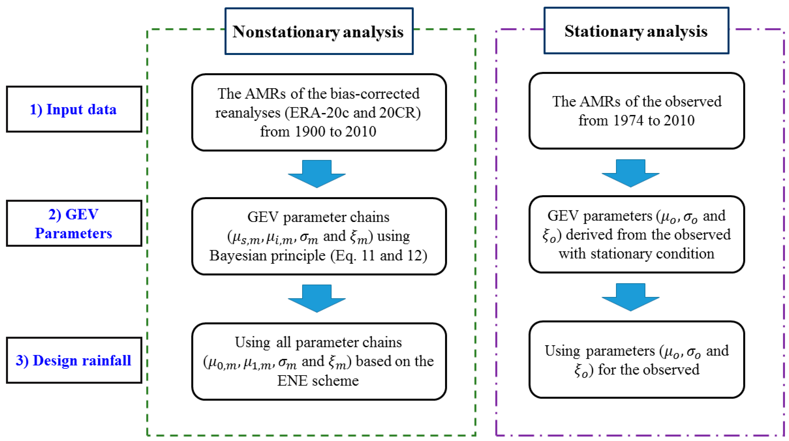
3.3. Rainfall Frequency Analysis with Nonstationary Condition

In hydrological models, time-varying parameter schemes have been commonly adopted for non-stationarity analysis in hydrometeorological applications [38,40,41,42,44,65]. As GEV family is typically applied for estimating IDFs in practice, we applied a GEV distribution with the time-varying location parameter ( μ t ), while scale ( σ ) and shape ( ξ ) parameters were set as constant. The location parameter is assumed as a time-depending linear function, and under the nonstationary condition.
To quantify the parameters for the GEV curve under nonstationary condition, we apply the Bayesian principle suggested by Cheng and AghaKouchak [1]. In this scheme, numerous parameter sets are estimated from the joint posterior distribution using the differential evolution Markov chain (DE-MC), which is based on the genetic algorithm differential evolution for global optimization with the Markov chain Monte Carlo (MCMC) principle [1].
With the time-varying parameter chains, the next step is to estimate the return period for a given design quantile under nonstationary condition. Numerous studies have dealt with the non-stationary interpretation, and there were two main approaches to handle it as (1) the expected waiting time (EWT) method and (2) the expected number of exceedance (ENE) method [42,44,45,47,66].
Both EWT and ENE are applicable for nonstationary events. However, as stated in the Introduction section, the EWT approach has a drawback of requiring infinite (or as long as possible) future exceedance probabilities in order to numerically solve the problem [42,47]. For this reason, we applied the ENE interpretation for estimating the design quantile with the return period from 10-year to 200-year (see Supplementary Material for more detail) (Figure 2).

4. Results

4.1. Bias Correction

To improve the uncorrected AMRs of ERA-20c and 20CR, we applied QM approaches based on three different distributions, gamma, Gumbel and GEV. The overall bias-corrected values over 48 stations for the reference period (1974–2010) were assessed by RMSE (mm) and NSE, as illustrated in Figure 3 and Table 2. Conceptually, the bias-corrected values by QDM and SQM methods with the same distribution are identical for the reference period. Thus, the outputs by three different distributions were denoted as gevQM, gamQM and gumQM. The overall comparison between the observed and the modelled indicated the significant reduction of errors in all QM schemes. The result showed that GEV distribution performed the best in both ERA-20c and 20CR. The bias-corrected ERA-20c by gevQM had 17.56 mm for RMSE and 0.924 for NSE, while the values by gamQM and gumQM were from 22.34 mm to 26.08 mm for RMSE and from 0.831 to 0.876 for NSE. For 20CR, the model efficiency by gevQM with 20.63 mm for RMSE and 0.894 for NSE dominated those by gamQM and gumQM with from 22.46 mm to 26.86 mm for RMSE and from 0.821 to 0.875 for NSE.
To spatially evaluate the performance, we also implemented the error estimation in individual stations, as shown in Figure 4 and Figure 5 for NSE and RMSE, respectively. Figure 4 illustrates NSE values for the AMRs of the bias-corrected ERA-20c and 20CR based on QM approaches (i.e., gevQM, gamQM and gumQM) in 48 stations, whereas Figure 5 indicates RMSE values. The model efficiencies were generally over 0.8 for NSE, in all model values except a few stations. For RMSE, the most error estimates were less than 30 mm, which indicates the significant reduction of the bias. To clearly analyze the range of the model values, we used a boxplot scheme based on the individual error estimates in 48 stations, as illustrated in Figure 6, and compared the mean values of the error estimation results in individual stations as described in Table 3. The boxplot for NSE in Figure 6a indicated that the median values were over 0.9 in all QM approaches and most values were within the range from 0.6 to 1. Especially, gevQM for ERA-20c showed the best efficiencies among three QM schemes, whereas for 20CR, gevQM and gamQM had a better performance than gumQM. The analysis on RMSE also showed the similar result (Figure 6b). The median values were generally within 10 to 15 mm in all bias-corrected values and gevQM for ERA-20c performed the best and gevQM for 20CR and gamQM for ERA-20c and 20CR closely followed. In terms of the mean, gevQM for ERA-20c showed the best efficiencies, with 14.30 mm for RMSE and 0.933 for NSE as described in Table 3. For 20CR, NSE values for gevQM and gamQM were similar but RMSE for gevQM, 16.69 mm, was slightly smaller than that of gamQM, 17.48 mm. These results suggest that the applied QM approaches can significantly reduce the error in the AMRs of reanalyses (i.e., ERA-20c and 20CR), and among three different transfer functions, GEV distribution could be the best option for bias correction of the AMRs, especially for ERA-20c.

4.2. Long-Term Trend

To consider the nonstationary condition in rainfall frequency analysis, the long-term trend of the AMRs should be necessarily detected. For this purpose, we analyzed the long-term trend of AMRs for the observed (Obs) and the bias corrected for the reference period (i.e., 1974–2010) using a non-parametric method, Mann–Kendall test as shown in Figure 7. To further evaluate the observed trend, we additionally analyzed the AMRs of the observation for the extended period, from 1974 to 2017 (Obs0). The results in both Obs and Obs0 had no significant trend at the 0.05 significant level except a few stations. More specifically, among 48 stations, only 5 stations for Obs and 2 stations for Obs0 presented significant trend, respectively. The performances for the bias-corrected reanalyses showed similar results. The AMRs of the bias-corrected reanalysis data (ERA-20c and 20CR) by QM approaches as well as the raw values (RAW) had no significant trends at the 0.05 significance level in all comparisons. Note that the recent 40 years’ data do not illustrate any significant data in the observation, as well as in the reanalysis data.
To estimate nonstationarity over the 20th century, we also checked a century-long trend using the bias corrected AMRs of ERA-20c and 20CR from 1900 to 2010, instead of the observation periods Obs and Obs0. Figure 8 illustrates the trend test results for the AMRs of the bias corrected reanalyses in 48 stations from 1900 to 2010. For ERA-20c, the corrected values by SQM approaches (gevSQM, gamSQM and gumSQM) had obvious increasing trends in all stations, and the QDM algorithms (gevQDM, gamQDM and gumQDM) also indicated the significant increasing trends at 0.05 significance level, except a few points. The results for 20CR were similar to those for ERA-20c. The bias-corrected values demonstrated the obvious increasing trends for both SQM and QDM schemes of the whole 20th century. These results imply that the AMRs in South Korea may have an increasing trend over the 20th century, although the AMRs in recent decades are not able to clarify the nonstationary characteristic.
To evaluate the magnitude of the trends, inter-annual variabilities over 48 stations from 1900 to 2010 were also analyzed as illustrated in Figure 9. Individual values for each station are presented with thin weak blue and red lines for ERA-20c and 20CR, respectively, while the means of 48 stations are presented with thick strong blue and red lines. Although there was the difference in specific movements between ERA-20c and 20CR, the trends of the overall means for 48 stations represented by bold blue color for ERA-20c and bold red color for 20CR illustrate the significant increasing trends for both cases.
The slopes for ERA-20c were within the range from 0.40 mm/year to 0.55 mm/year, whereas 20CR had fewer slopes from 0.34 to 0.45 mm/year as described in Table 4. In comparison between SQM and QDM approaches, the trends by QDM schemes were lower than those by the corresponding SQM methods in both ERA-20c and 20CR. With the assumption that two reanalyses, ERA-20c and 20CR, could substantially reproduce the long-term trend, these temporal patterns imply the clear non-stationarity of the AMRs in South Korea from 1900 to 2010.
It is surprising that the slopes of all stations based on the two different reanalysis products present a similar increasing trend. This result implies that the extreme data over South Korea might have a significant increasing trend that the current observed data with the limited period such as 1974–2010 and 1974–2017 cannot capture. Therefore, the abstraction of these trends might be beneficial in estimating the future extreme design rainfall over South Korea with nonstationary frequency analysis. The following study was conducted accordingly to employ the derived overall trend that might be more feasible to occur in nature, even though a certain degree of uncertainties is included.

4.3. Design Rainfalls with Nonstationary Condition

To explore design rainfalls with the nonstationary condition by using the bias-corrected AMRs from 1900 to 2010, we estimated time-varying parameters of GEV distribution. Nonstationary design rainfalls were estimated by the BM approach based on the GEV parameters ( μ s , m ,   μ i , m ,   σ m and ξ m ) derived from the bias-corrected AMRs. Here, the bias-corrected AMRs were collected from QM approaches with GEV distribution (gevSQM and gevQDM), which showed the best performance in Section 4.1.
To find out the impact of nonstationary condition, we representatively illustrated design rainfall comparisons in the selected 4 stations, St.5, St.18, St.21, and St.27 in Figure 10. In the comparisons, design quantiles showed the significant range of uncertainties, which had an upper-bound of approximately 1.3 to 2.0 times higher than the design rainfalls by the observed and a lower bound of about 7–45% lower. For example, for St.5 Seoul, the precipitation quantiles with 100-year return period derived from ERA-20C varied from about 327 mm to 815 mm for gevSQM, and from 346 mm to 852 mm for gevQDM, while the classic quantile by the observation was 483 mm. This characteristic is also shown in the other stations.
For the median values, the design quantiles of the reanalyses with long return periods such as 100-year and 200-year were generally higher than those by the observations except st.21 Busan, while the design rainfalls with short return periods, i.e., 10-year and 20-year, have little difference from the observed. For instance, St.18 Jeonju had a small gap in 10-year design quantiles between the observation and the reanalyses, but the longer the return period, the more gap there exists, especially for ERA-20c. St.5 Seoul and St.27 Inje also showed a similar characteristic, with the design rainfall for the reanalyses exceeding those for the observed as the return period became longer. On the other hand, St.21 Busan had no clear feature compared with the other stations, and even the design rainfall for the observed exceeded those by the bias-corrected reanalyses for gevSQM. Although reanalysis products-based design rainfall estimation includes a certain degree of uncertainty, these results imply that the nonstationary design rainfall would influence on estimating the future risk of extreme precipitation and the strength of the impact depends on the target return period and location.
To find out the spatial influence of non-stationarity in design rainfall, we estimated the relative change (%) of design rainfall with 100-year return period based on the median values of the generated parameter chains in 48 stations. The relative change in 48 stations varied from −38.1% to 58.4% for gevSQM, and from −30.8% to 42.8% for gevQDM, respectively, but the spatial comparisons in Figure 11 illustrated the increase of the relative change (%) in many regions over South Korea.
Furthermore, the spatial area presenting lower or higher than the observed quantiles is more similar in case of the QDM for ERA-20c and 20CR than SQM. The results of the gevQDM relative change shown at the bottom panels of Figure 11 present that the southern and middle regions have higher design rainfall estimation than the observed one, while the northern region and the edge of the southeast and southwest present lower design rainfall from the gevQDM than from the observed one.
Despite the uncertainty range, this result suggests that the conventional stationary approach based on the multi-decadal observation may lead to significant underestimation of future risk in some regions. For example, southwest parts within 35–36° N and 126.5–127.5° E had relative change within approximately 10% to 50% in all comparisons. It is obvious that there still exists a certain degree of errors in design rainfall taken from the bias-corrected reanalyses. Nevertheless, if practitioners want to design a project but only have a limited observation, this result can provide meaningful information for a project plan with long-term life span.

5. Discussion

Despite the meaningful information, the proposed method inevitably contains errors from various reasons. Basically, long-term reanalyses for daily precipitation have the systematic errors that spatio-temporally vary [17,20,67,68,69]. Previous studies have documented that century-long reanalyses like ERA-20c and 20CR are able to mislead long-term trends and the bias may considerably exist for the first half of the twentieth century [16,70,71,72,73]. The proposed bias correction methods, SQM and QDM, also have a limitation. As a QM approach cannot exactly correct the climate change trend [23], the potential error in the long-term trend of the raw data may propagate the bias into the bias corrected value. Moreover, a QM approach based on a certain distribution such as gamma can underestimate highly extreme rainfalls, which are mainly described by the upper tail of the distribution [55,74,75,76]. Thus, some studied have introduced a combination or mixture distribution like gamma-Pareto to better reproduce the heavy tail [24,55,77,78]. The scale gap between the observed and the modelled can result in the biases [79]. In other words, as the proposed QM approaches matched the transfer function between the observation with point-scale and the model data with grid-scale, the bias-corrected value may include errors.
In design rainfall estimation with nonstationary condition, how to define time-varying parameters is also one major issue. We assume a linearly time-dependent location parameter, which is commonly adopted in nonstationary studies, but several studies have also suggested non-linear location parameter or time-varying scale parameter [1,35,38,40,41,43,46,59,66].
Likewise, various causes may result in substantial errors for the design rainfall interpretation in this study. Nevertheless, the proposed analysis suggests meaningful information to help to forecast future risk under the climate change environment. As rainfall intensity is expected to increase in the future, the conventional approach with stationary assumption may underestimate future risk. Several studies and authorities have suggested the guideline for design rainfall and design flood considering the potential impact [80,81,82]. However, these guidelines typically suggest adding a correction factor into design rainfall or design flood estimated under stationary condition [81]. For instance, the agency [82] recommended increasing the peak rainfall intensity from 5% to 40% for the future period (2015–2115), compared with the data for the baseline period (1961–1990). However, those suggestions are generally based on the analysis of future climate change scenarios which also include significant biases, and the nonstationary analysis based on the observation is constrained by lack of data. Thus, despite the substantial errors, the proposed approach in this study can be a considerable option to achieve additional information for estimating future risk in rainfall.

6. Summary and Conclusions

In this study, we aimed to explore design rainfalls under nonstationary condition by using century-long reanalyses, ERA-20 and 20CR, over South Korea. For this purpose, we first improved the AMRs of the reanalyses from 1900 to 2010 by using a trend-preserving method, QDM, compared with the conventional stationary QM scheme, SQM. After bias correction, we assessed the long-term trend of the bias-corrected AMRs for the whole 20th century to confirm the nonstationarity. With the improved values of ERA-20c and 20CR, we estimated design rainfalls under nonstationary condition based on the ENE approach in 48 stations. Finally, we also explored the spatial change in design rainfalls between the applied nonstationary approach in the current study and the conventional approach. The major results obtained in this study are summarized as follows:
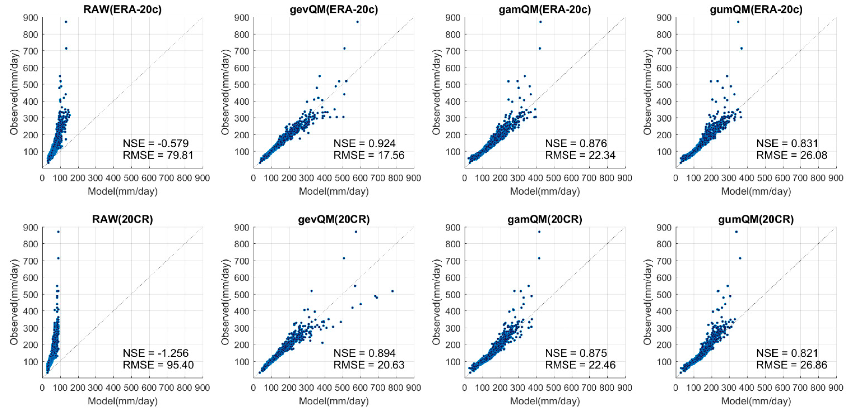
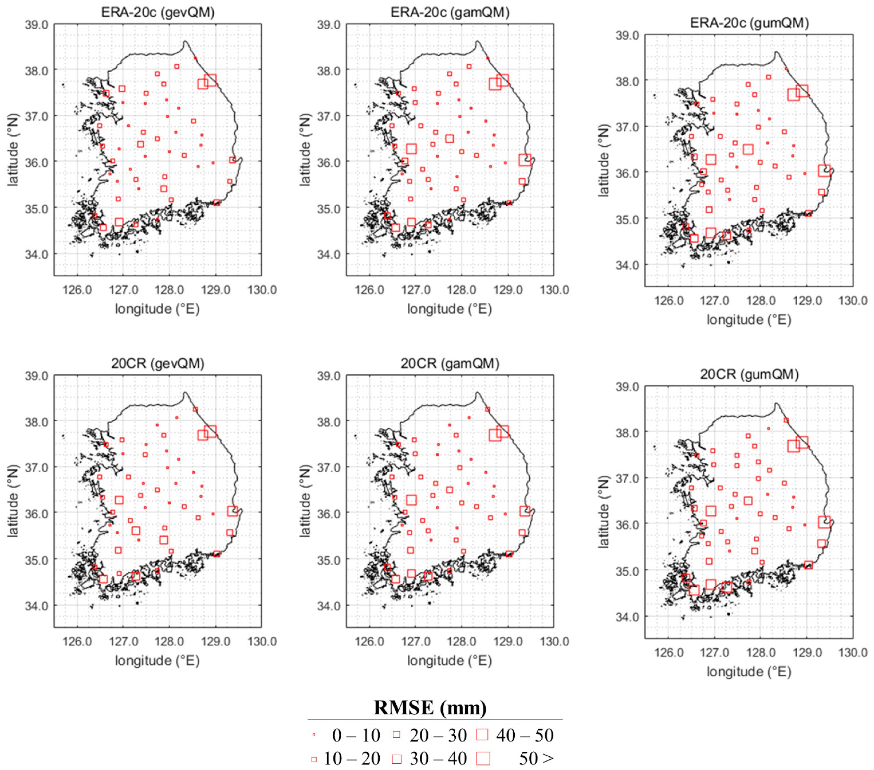
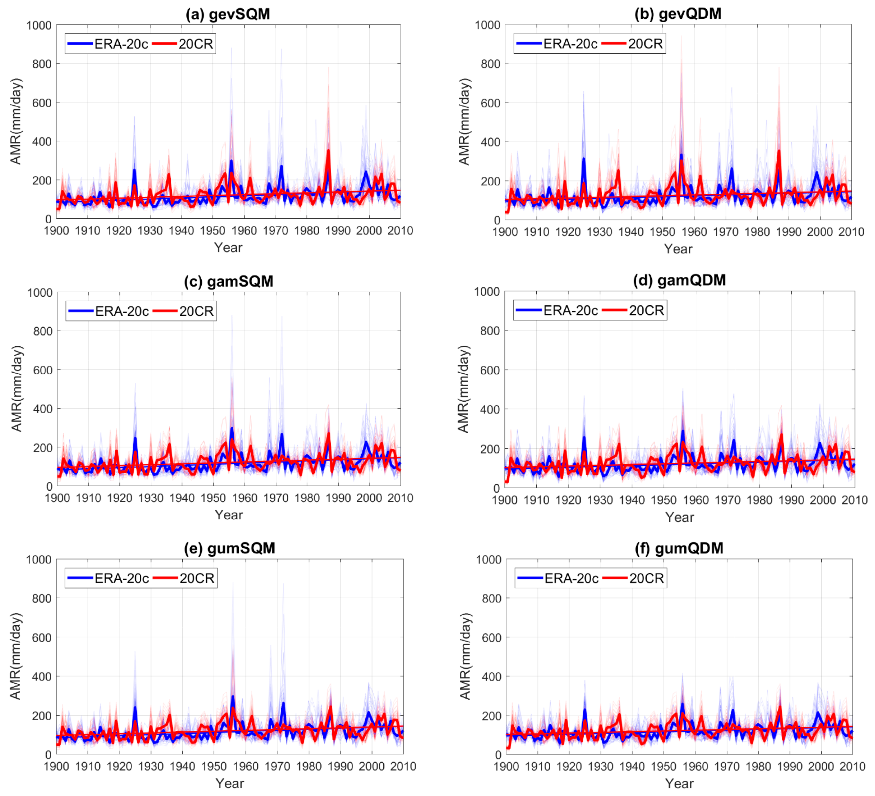
  • The applied QM approaches (gevQM, gamQM and gumQM) significantly improved the AMRs of ERA-20c and 20CR for the reference period. Among three QM schemes, gevQM performed the best in terms of RMSE and NSE.
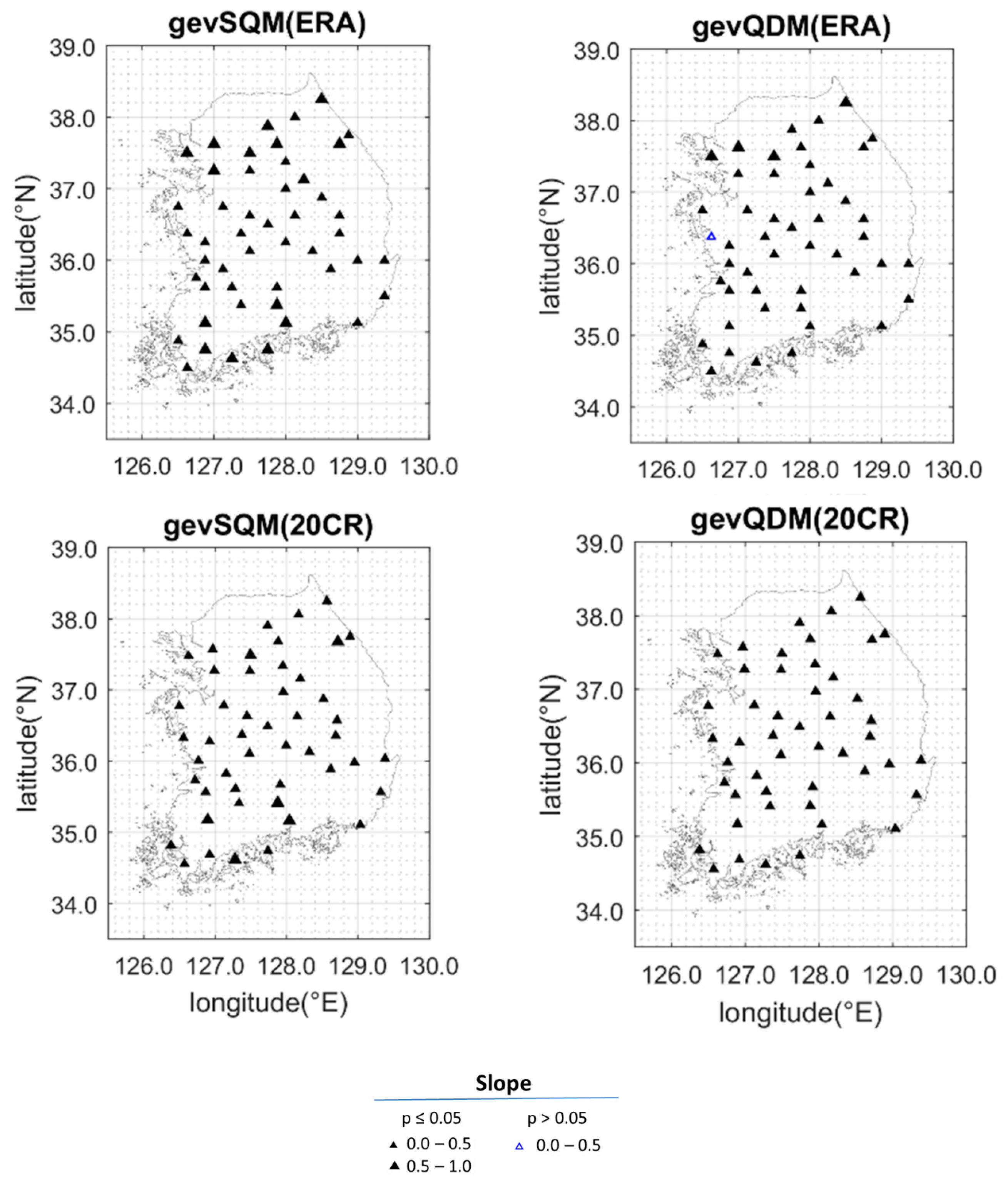
  • For long-term trend, no significant trend for the AMRs of the observed and the reanalyses can be found during the observational period. However, the century-long AMRs of the bias corrected ERA-20c and 20CR indicated the increasing trends. This result implies that the AMRs might have time-dependent characteristics and the trend in the long-term reanalysis datasets could be beneficial in estimating the future extreme design rainfall over South Korea with nonstationary frequency analysis.
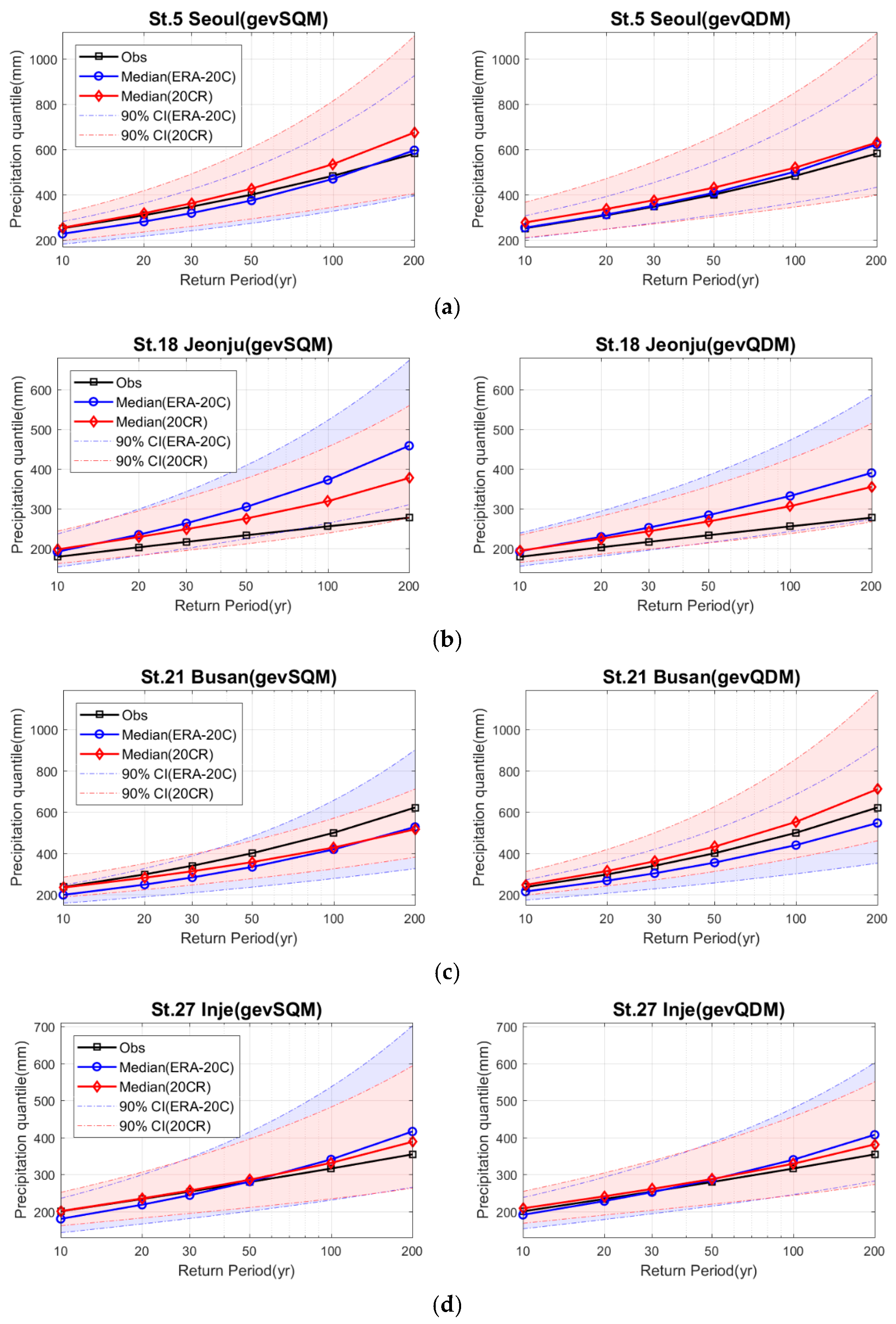
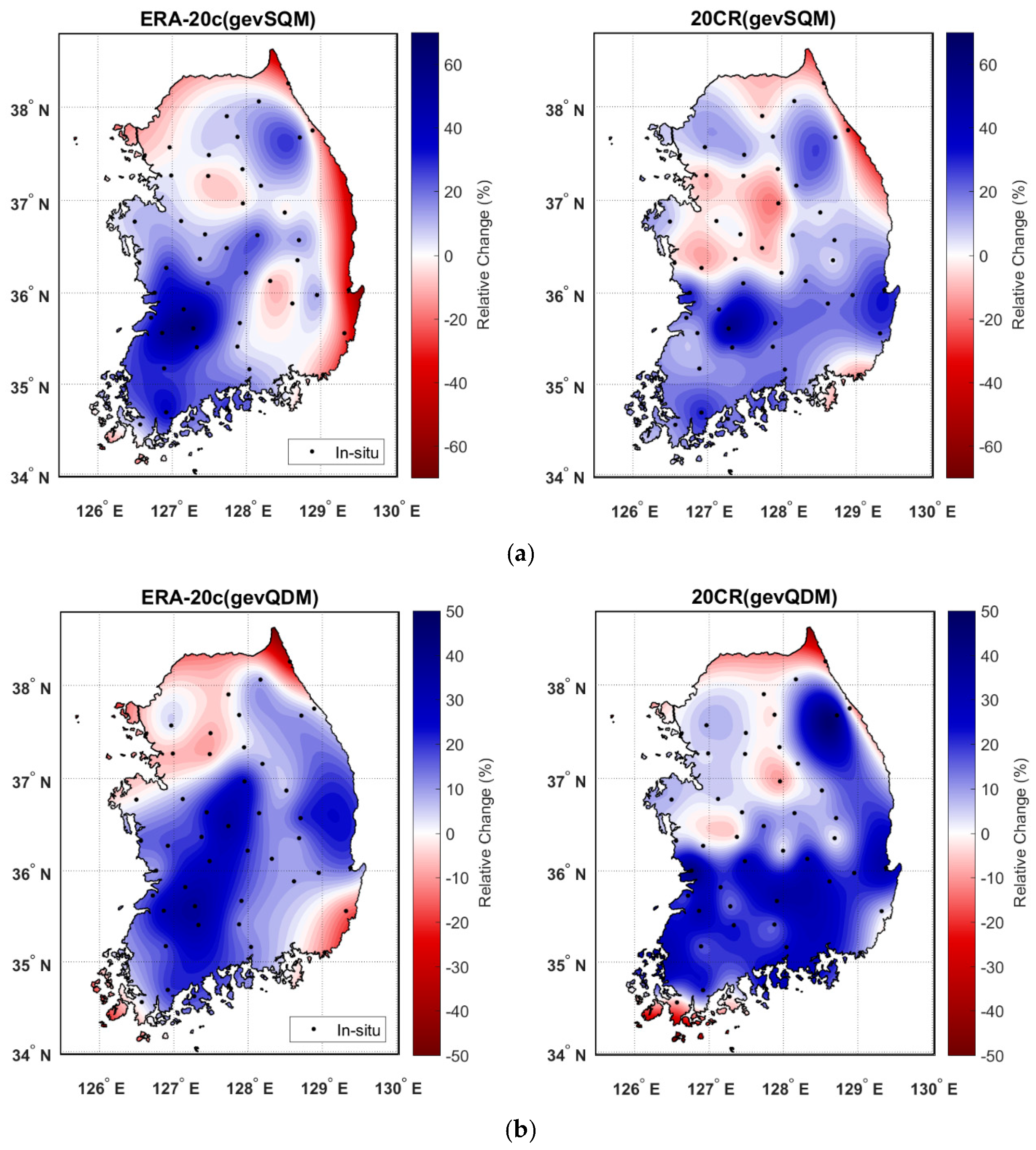
  • The design rainfalls estimated under nonstationary condition were influenced in estimating the future risk of extreme precipitation and the strength of the impact depends on the target return period and location. More specifically, the nonstationary design rainfalls in some parts of South Korea exceeded the classic design rainfalls by the observed. This result implies that the nonstationarity in the AMRs that the short-term observation often fails to detect could deteriorate the confidence of a project based on the observed data for the future risk in South Korea.
The findings obtained in this study provide a meaningful perspective on the applicability of century-long reanalysis products, especially for nonstationary rainfall frequency analysis in a region with a limited observation network. Despite a certain degree of errors, the proposed scheme with employing the reanalysis products can be beneficial to predict the future evolution of extreme precipitation and to estimate the design rainfall accordingly.

Supplementary Materials

The following are available online at https://www.mdpi.com/2073-4433/12/2/191/s1. Figure S1. A flow chart for estimating design rainfall under the conditions of nonstationarity and stationarity.

Author Contributions

Methodology, D.-I.K. and T.L.; Project administration, D.H.; Writing—original draft, D.-I.K.; Writing—review & editing, T.L. All authors have read and agreed to the published version of the manuscript.

Funding

The first author is funded by the Government of South Korea for performing his doctoral studies at the University of Bristol. The third author acknowledges the support of the National Research Foundation of Korea (NRF) grant (2018R1A2B600179), funded by the Korean Government (MEST).

Institutional Review Board Statement

Not applicable.

Informed Consent Statement

Not applicable.

Data Availability Statement

Not applicable.

Acknowledgments

We are grateful for the relevant data provided by KMA, ECMWF and NCAA.

Conflicts of Interest

The authors declare no conflict of interest.

References

  1. Cheng, L.; Aghakouchak, A. Nonstationary precipitation intensity-duration-frequency curves for infrastructure design in a changing climate. Sci. Rep. 2014, 4, 1–6. [Google Scholar] [CrossRef] [PubMed] [Green Version]
  2. Li, J.; Evans, J.; Johnson, F.; Sharma, A. A comparison of methods for estimating climate change impact on design rainfall using a high-resolution RCM. J. Hydrol. 2017, 547, 413–427. [Google Scholar] [CrossRef]
  3. Alexander, L.V.; Zhang, X.; Peterson, T.C.; Caesar, J.; Gleason, B.; Klein Tank, A.M.G.; Haylock, M.; Collins, D.; Trewin, B.; Rahimzadeh, F.; et al. Global observed changes in daily climate extremes of temperature and precipitation. J. Geophys. Res. Atmos. 2006, 111, 1–22. [Google Scholar] [CrossRef] [Green Version]
  4. IPCC. Climate Change 2014–Impacts, Adaptation and Vulnerability: Regional Aspects; Cambridge University Press: London, UK, 2014. [Google Scholar]
  5. De Luca, D.L.; Galasso, L. Stationary and non-stationary frameworks for extreme rainfall time series in southern Italy. Water 2018, 10, 1477. [Google Scholar] [CrossRef] [Green Version]
  6. Coles, S.; Pericchi, L.R.; Sisson, S. A fully probabilistic approach to extreme rainfall modeling. J. Hydrol. 2003, 273, 35–50. [Google Scholar] [CrossRef]
  7. Overeem, A.; Buishand, A.; Holleman, I. Rainfall depth-duration-frequency curves and their uncertainties. J. Hydrol. 2008, 348, 124–134. [Google Scholar] [CrossRef]
  8. Huard, D.; Mailhot, A.; Duchesne, S. Bayesian estimation of intensity-duration-frequency curves and of the return period associated to a given rainfall event. Stoch. Environ. Res. Risk Assess. 2010, 24, 337–347. [Google Scholar] [CrossRef]
  9. Tung, Y.K.; Wong, C.L. Assessment of design rainfall uncertainty for hydrologic engineering applications in Hong Kong. Stoch. Environ. Res. Risk Assess. 2014, 28, 583–592. [Google Scholar] [CrossRef]
  10. Van de Vyver, H. Bayesian estimation of rainfall intensity-duration-frequency relationships. J. Hydrol. 2015, 529, 1451–1463. [Google Scholar] [CrossRef]
  11. Serinaldi, F.; Kilsby, C.G. Stationarity is undead: Uncertainty dominates the distribution of extremes. Adv. Water Resour. 2015, 77, 17–36. [Google Scholar] [CrossRef] [Green Version]
  12. Koutsoyiannis, D.; Montanari, A. Negligent killing of scientific concepts: The stationarity case. Hydrol. Sci. J. 2015, 60, 1174–1183. [Google Scholar] [CrossRef]
  13. Dee, D.P.; Uppala, S.M.; Simmons, A.J.; Berrisford, P.; Poli, P.; Kobayashi, S.; Andrae, U.; Balmaseda, M.A.; Balsamo, G.; Bauer, P. The ERA-Interim reanalysis: Configuration and performance of the data assimilation system. Q. J. R. Meteorol. Soc. 2011, 137, 553–597. [Google Scholar] [CrossRef]
  14. Zhang, Q.; Körnich, H.; Holmgren, K. How well do reanalyses represent the southern African precipitation? Clim. Dyn. 2013, 40, 951–962. [Google Scholar] [CrossRef]
  15. Hersbach, H.; Peubey, C.; Simmons, A.; Berrisford, P.; Poli, P.; Dee, D. ERA-20CM: A twentieth-century atmospheric model ensemble. Q. J. R. Meteorol. Soc. 2015, 141, 2350–2375. [Google Scholar] [CrossRef]
  16. Donat, M.G.; Alexander, L.V.; Herold, N.; Dittus, A.J. Temperature and precipitation extremes in century-long gridded observations, reanalyses, and atmospheric model simulations. J. Geophys. Res. Atmos. 2016, 121, 11174–11189. [Google Scholar] [CrossRef] [Green Version]
  17. Gao, L.; Bernhardt, M.; Schulz, K.; Chen, X.W.; Chen, Y.; Liu, M.B. A First Evaluation of ERA-20CM over China. Mon. Weather Rev. 2016, 144, 45–57. [Google Scholar] [CrossRef]
  18. Poli, P.; Hersbach, H.; Dee, D.P.; Berrisford, P.; Simmons, A.J.; Vitart, F.; Laloyaux, P.; Tan, D.G.H.; Peubey, C.; Thépaut, J.-N. ERA-20C: An Atmospheric Reanalysis of the Twentieth Century. J. Clim. 2016, 29, 4083–4097. [Google Scholar] [CrossRef]
  19. Compo, G.P.; Whitaker, J.S.; Sardeshmukh, P.D.; Matsui, N.; Allan, R.J.; Yin, X.; Gleason, B.E.; Vose, R.S.; Rutledge, G.; Bessemoulin, P. The twentieth century reanalysis project. Q. J. R. Meteorol. Soc. 2011, 137, 1–28. [Google Scholar] [CrossRef]
  20. Kim, D.-I.; Han, D. Comparative study on long term climate data sources over South Korea. J. Water Clim. Chang. 2018, (in press). [Google Scholar] [CrossRef] [Green Version]
  21. Teutschbein, C.; Seibert, J. Bias correction of regional climate model simulations for hydrological climate-change impact studies: Review and evaluation of different methods. J. Hydrol. 2012, 456, 12–29. [Google Scholar] [CrossRef]
  22. Mao, G.; Vogl, S.; Laux, P.; Wagner, S.; Kunstmann, H. Stochastic bias correction of dynamically downscaled precipitation fields for Germany through Copula-based integration of gridded observation data. Hydrol. Earth Syst. Sci. 2015, 19, 1787–1806. [Google Scholar] [CrossRef] [Green Version]
  23. Maraun, D. Bias Correcting Climate Change Simulations—A Critical Review. Curr. Clim. Chang. Rep. 2016, 2, 211–220. [Google Scholar] [CrossRef] [Green Version]
  24. Nyunt, C.T.; Koike, T.; Yamamoto, A. Statistical bias correction for climate change impact on the basin scale precipitation in Sri Lanka, Philippines, Japan and Tunisia. Hydrol. Earth Syst. Sci. 2016. [Google Scholar] [CrossRef]
  25. Themeßl, M.J.; Gobiet, A.; Heinrich, G. Empirical-statistical downscaling and error correction of regional climate models and its impact on the climate change signal. Clim. Chang. 2012, 112, 449–468. [Google Scholar] [CrossRef]
  26. Fang, G.; Yang, J.; Chen, Y.N.; Zammit, C. Comparing bias correction methods in downscaling meteorological variables for a hydrologic impact study in an arid area in China. Hydrol. Earth Syst. Sci. 2015, 19, 2547–2559. [Google Scholar] [CrossRef] [Green Version]
  27. Maraun, D.; Widmann, M. Statistical Downscaling and Bias Correction for Climate Research; Cambridge University Press: London, UK, 2018; pp. 170–200. [Google Scholar]
  28. Chang, H.; Kwon, W.-T. Spatial variations of summer precipitation trends in South Korea, 1973–2005. Environ. Res. Lett. 2007, 2, 45012. [Google Scholar] [CrossRef] [Green Version]
  29. Choi, G.; Collins, D.; Ren, G.; Trewin, B.; Baldi, M.; Fukuda, Y.; Afzaal, M.; Pianmana, T.; Gomboluudev, P.; Huong, P.T.T. Changes in means and extreme events of temperature and precipitation in the Asia-Pacific Network region, 1955–2007. Int. J. Climatol. 2009, 29, 1906–1925. [Google Scholar] [CrossRef]
  30. Jung, I.W.; Bae, D.H.; Kim, G. Recent trends of mean and extreme precipitation in Korea. Int. J. Climatol. 2011, 31, 359–370. [Google Scholar] [CrossRef]
  31. Cannon, A.J.; Sobie, S.R.; Murdock, T.Q. Bias correction of GCM precipitation by quantile mapping: How well do methods preserve changes in quantiles and extremes? J. Clim. 2015, 28, 6938–6959. [Google Scholar] [CrossRef]
  32. Miao, C.; Su, L.; Sun, Q.; Duan, Q. A nonstationary bias-correction technique to remove bias in GCM simulations. J. Geophys. Res. 2016, 121, 5718–5735. [Google Scholar] [CrossRef]
  33. Eum, H.I.; Cannon, A.J. Intercomparison of projected changes in climate extremes for South Korea: Application of trend preserving statistical downscaling methods to the CMIP5 ensemble. Int. J. Climatol. 2017, 37, 3381–3397. [Google Scholar] [CrossRef]
  34. Nahar, J.; Johnson, F.; Sharma, A. Assessing the extent of non-stationary biases in GCMs. J. Hydrol. 2017, 549, 148–162. [Google Scholar] [CrossRef] [Green Version]
  35. Nadarajah, S.; Choi, D. Maximum daily rainfall in South Korea. J. Earth Syst. Sci. 2007, 116, 311–320. [Google Scholar] [CrossRef]
  36. Cunderlik, J.M.; Burn, D.H. Non-stationary pooled flood frequency analysis. J. Hydrol. 2003, 276, 210–223. [Google Scholar] [CrossRef]
  37. El Adlouni, S.; Ouarda, T.B.M.J.; Zhang, X.; Roy, R.; Bobée, B. Generalized maximum likelihood estimators for the nonstationary generalized extreme value model. Water Resour. Res. 2007, 43, 1–13. [Google Scholar] [CrossRef]
  38. Leclerc, M.; Ouarda, T.B.M.J. Non-stationary regional flood frequency analysis at ungauged sites. J. Hydrol. 2007, 343, 254–265. [Google Scholar] [CrossRef]
  39. Cannon, A.J. A flexible nonlinear modelling framework for nonstationary generalized extreme value analysis in hydroclimatology. Hydrol. Process. 2010, 24, 673–685. [Google Scholar] [CrossRef]
  40. Panagoulia, D.; Economou, P.; Caroni, C. Stationary and nonstationary generalized extreme value modelling of extreme precipitation over a mountainous area under climate change. Environmetrics 2014, 25, 29–43. [Google Scholar] [CrossRef]
  41. Son, C.; Lee, T.; Kwon, H.H. Integrating nonstationary behaviors of typhoon and non-typhoon extreme rainfall events in East Asia. Sci. Rep. 2017, 7, 1–9. [Google Scholar] [CrossRef] [Green Version]
  42. Du, T.; Xiong, L.; Xu, C.Y.; Gippel, C.J.; Guo, S.; Liu, P. Return period and risk analysis of nonstationary low-flow series under climate change. J. Hydrol. 2015, 527, 234–250. [Google Scholar] [CrossRef] [Green Version]
  43. Cheng, L.; AghaKouchak, A.; Gilleland, E.; Katz, R.W. Non-stationary extreme value analysis in a changing climate. Clim. Chang. 2014, 127, 353–369. [Google Scholar] [CrossRef]
  44. Salas, J.D.; Obeysekera, J. Revisiting the Concepts of Return Period and Risk for Nonstationary Hydrologic Extreme Events. J. Hydrol. Eng. 2014, 19, 554–568. [Google Scholar] [CrossRef] [Green Version]
  45. Read, L.K.; Vogel, R.M. Reliability, return periods, and risk under nonstationarity. Water Resour. Res. 2015, 51, 6381–6398. [Google Scholar] [CrossRef]
  46. Obeysekera, J.; Salas, J.D. Frequency of Recurrent Extremes under Nonstationarity. J. Hydrol. Eng. 2016, 21, 1–9. [Google Scholar] [CrossRef]
  47. Salas, J.D.; Obeysekera, J.; Vogel, R.M. Techniques for assessing water infrastructure for nonstationary extreme events: A review. Hydrol. Sci. J. 2018, 63, 325–352. [Google Scholar] [CrossRef]
  48. Berntell, E.; Zhang, Q.; Chafik, L.; Körnich, H. Representation of Multidecadal Sahel Rainfall Variability in 20th Century Reanalyses. Sci. Rep. 2018, 8. [Google Scholar] [CrossRef] [Green Version]
  49. Diro, G.T.; Grimes, D.I.F.; Black, E.; O’Neill, A.; Pardo-Iguzquiza, E. Evaluation of reanalysis rainfall estimates over Ethiopia. Int. J. Climatol. 2009, 29, 67–78. [Google Scholar] [CrossRef]
  50. Hu, Q.; Li, Z.; Wang, L.; Huang, Y.; Wang, Y.; Li, L. Rainfall spatial estimations: A review from spatial interpolation to multi-source data merging. Water 2019, 11, 579. [Google Scholar] [CrossRef] [Green Version]
  51. Hua, W.; Zhou, L.; Nicholson, S.E.; Chen, H.; Qin, M. Assessing reanalysis data for understanding rainfall climatology and variability over Central Equatorial Africa. Clim. Dyn. 2019, 53, 651–669. [Google Scholar] [CrossRef] [Green Version]
  52. Kim, K.B.; Bray, M.; Han, D. An improved bias correction scheme based on comparative precipitation characteristics. Hydrol. Process. 2015, 29, 2258–2266. [Google Scholar] [CrossRef] [Green Version]
  53. Rabiei, E.; Haberlandt, U. Applying bias correction for merging rain gauge and radar data. J. Hydrol. 2015, 522, 544–557. [Google Scholar] [CrossRef]
  54. Kim, K.B.; Kwon, H.H.; Han, D. Bias correction methods for regional climate model simulations considering the distributional parametric uncertainty underlying the observations. J. Hydrol. 2015, 530, 568–579. [Google Scholar] [CrossRef] [Green Version]
  55. Volosciuk, C.; Maraun, D.; Vrac, M.; Widmann, M. A combined statistical bias correction and stochastic downscaling method for precipitation. Hydrol. Earth Syst. Sci. 2017, 21, 1693–1719. [Google Scholar] [CrossRef] [Green Version]
  56. Koutsoyiannis, D. Statistics of extremes and estimation of extreme rainfall: I. Theoretical investigation. Hydrol. Sci. J. 2004, 49, 575–590. [Google Scholar] [CrossRef] [Green Version]
  57. Wilson, P.S.; Toumi, R. A fundamental probability distribution for heavy rainfall. Geophys. Res. Lett. 2005, 32, 1–4. [Google Scholar] [CrossRef]
  58. Li, H.; Sheffield, J.; Wood, E.F. Bias correction of monthly precipitation and temperature fields from Intergovernmental Panel on Climate Change AR4 models using equidistant quantile matching. J. Geophys. Res. Atmos. 2010, 115, 1–20. [Google Scholar] [CrossRef]
  59. Bürger, G.; Sobie, S.R.; Cannon, A.J.; Werner, A.T.; Murdock, T.Q. Downscaling extremes: An intercomparison of multiple methods for future climate. J. Clim. 2013, 26, 3429–3449. [Google Scholar] [CrossRef]
  60. Hamed, K.H.; Rao, A.R. A modified Mann-Kendall trend test for autocorrelated data. J. Hydrol. 1998, 204, 182–196. [Google Scholar] [CrossRef]
  61. Sen, P.K. Estimates of the regression coefficient based on Kendall’s tau. J. Am. Stat. Assoc. 1968, 63, 1379–1389. [Google Scholar] [CrossRef]
  62. Theil, H. A rank-invariant method of linear and polynomial regression analysis. I, II, III. Proc. K. Ned. Akad. Wet. 1950, 53, 386–392, 521–525, 1397–1412. [Google Scholar]
  63. Sayemuzzaman, M.; Jha, M.K. Seasonal and annual precipitation time series trend analysis in North Carolina, United States. Atmos. Res. 2014, 137, 183–194. [Google Scholar] [CrossRef]
  64. Shadmani, M.; Marofi, S.; Roknian, M. Trend analysis in reference evapotranspiration using Mann-Kendall and Spearman’s Rho tests in arid regions of Iran. Water Resour. Manag. 2012, 26, 211–224. [Google Scholar] [CrossRef] [Green Version]
  65. Ouarda, T.B.M.J.; El-Adlouni, S. Bayesian nonstationary frequency analysis of hydrological variables. J. Am. Water Resour. Assoc. 2011, 47, 496–505. [Google Scholar] [CrossRef]
  66. Obeysekera, J.; Salas, J.D. Quantifying the Uncertainty of Design Floods under Nonstationary Conditions. J. Hydrol. Eng. 2014, 19, 1438–1446. [Google Scholar] [CrossRef]
  67. Bosilovich, M.G.; Chen, J.; Robertson, F.R.; Adler, R.F. Evaluation of global precipitation in reanalyses. J. Appl. Meteorol. Climatol. 2008, 47, 2279–2299. [Google Scholar] [CrossRef]
  68. Ma, L.; Zhang, T.; Frauenfeld, O.W.; Ye, B.; Yang, D.; Qin, D. Evaluation of precipitation from the ERA-40, NCEP-1, and NCEP-2 Reanalyses and CMAP-1, CMAP-2, and GPCP-2 with ground-based measurements in China. J. Geophys. Res. Atmos. 2009, 114, 1–20. [Google Scholar] [CrossRef]
  69. Bao, X.; Zhang, F. Evaluation of NCEP–CFSR, NCEP–NCAR, ERA-Interim, and ERA-40 reanalysis datasets against independent sounding observations over the Tibetan Plateau. J. Clim. 2013, 26, 206–214. [Google Scholar] [CrossRef] [Green Version]
  70. Brands, S.; Gutiérrez, J.M.; Herrera, S.; Cofiño, A.S. On the use of reanalysis data for downscaling. J. Clim. 2012, 25, 2517–2526. [Google Scholar] [CrossRef] [Green Version]
  71. Krueger, O.; Schenk, F.; Feser, F.; Weisse, R. Inconsistencies between long-term trends in storminess derived from the 20CR reanalysis and observations. J. Clim. 2013, 26, 868–874. [Google Scholar] [CrossRef] [Green Version]
  72. Poli, P.; Hersbach, H.; Tan, D.; Dee, D.; Thépaut, J.-N.; Simmons, A.; Peubey, C.; Laloyaux, P.; Komori, T.; Berrisford, P.; et al. The data assimilation system and initial performance evaluation of the ECMWF pilot reanalysis of the 20th-century assimilating surface observations only (ERA-20C). ERA Rep. Ser. 2013, 14, 59. [Google Scholar]
  73. Befort, D.J.; Wild, S.; Kruschke, T.; Ulbrich, U.; Leckebusch, G.C. Different long-term trends of extra-tropical cyclones and windstorms in ERA-20C and NOAA-20CR reanalyses. Atmos. Sci. Lett. 2016, 17, 586–595. [Google Scholar] [CrossRef] [Green Version]
  74. Wilks, D.S. Interannual variability and extreme-value characteristics of several stochastic daily precipitation models. Agric. For. Meteorol. 1999, 93, 153–169. [Google Scholar] [CrossRef]
  75. Vrac, M.; Naveau, P. Stochastic downscaling of precipitation: From dry events to heavy rainfalls. Water Resour. Res. 2007, 43, 1–13. [Google Scholar] [CrossRef] [Green Version]
  76. Hundecha, Y.; Pahlow, M.; Schumann, A. Modeling of daily precipitation at multiple locations using a mixture of distributions to characterize the extremes. Water Resour. Res. 2009, 45, 1–15. [Google Scholar] [CrossRef] [Green Version]
  77. Gutjahr, O.; Heinemann, G. Comparing precipitation bias correction methods for high-resolution regional climate simulations using COSMO-CLM. Theor. Appl. Climatol. 2013, 114, 511–529. [Google Scholar] [CrossRef]
  78. Smith, A.; Freer, J.; Bates, P.; Sampson, C. Comparing ensemble projections of flooding against flood estimation by continuous simulation. J. Hydrol. 2014, 511, 205–219. [Google Scholar] [CrossRef] [Green Version]
  79. Maraun, D. Bias Correction, Quantile Mapping, and Downscaling: Revisiting the Inflation Issue. J. Clim. 2013, 26, 2013–2014. [Google Scholar] [CrossRef] [Green Version]
  80. Lawrence, D.; Hisdal, H. Hydrological Projections for Floods in Norway under a Future Climate; Norwegian Water Resources and Energy Directorate: Oslo, Norway, 2011; p. 47.
  81. Madsen, H.; Lawrence, D.; Lang, M.; Martinkova, M.; Kjeldsen, T.R. Review of trend analysis and climate change projections of extreme precipitation and floods in Europe. J. Hydrol. 2014, 519, 3634–3650. [Google Scholar] [CrossRef] [Green Version]
  82. Flood Risk Assessments: Climate Change Allowances. 2017. Available online: https://www.gov.uk/guidance/flood-risk-assessments-climate-change-allowances (accessed on 31 January 2020).
Figure 1. A map showing the study area, local gauging stations, grid points of ERA-20c and 20CR. The grey shading on the map indicates elevations.
Atmosphere 12 00191 g001
Figure 2. A flow chart for estimating design rainfall with the nonstationary condition and stationary condition (see Supplementary Material for the detailed equations).
Atmosphere 12 00191 g002
Figure 3. Scatter plots between the annual maximum rainfalls (AMRs) of the observation and the model data (the raw reanalyses (RAW(ERA-20c) and RAW (20CR)) and the bias-corrected reanalyses (i.e., ERA-20c and 20CR) by the quantile mapping (QM) approaches with generalized extreme value (GEV), gamma and Gumbel distributions (gevQM, gamQM and gumQM)) over 48 stations, from 1974 to 2010.
Atmosphere 12 00191 g003
Figure 4. Mapping Nash–Sutcliffe efficiency (NSE) for the AMRs of the bias corrected ERA-20c (above) and 20CR (bottom) by QM approach (gevQM) in 48 stations for the reference period (1974–2010).
Atmosphere 12 00191 g004
Figure 5. Root mean square error (RMSE) for the AMRs of the bias corrected ERA-20c (above) and 20CR (bottom) by QM approach (gevQM) in 48 stations for the reference period (1974–2010).
Atmosphere 12 00191 g005
Figure 6. Boxplots of (a) NSE and (b) RMSE (mm) results for the AMRs of the bias corrected ERA-20c (ERA) and 20CR by QM approaches using three different distributions, GEV (gev), gamma (gam), and Gumbel (gum) in 48 stations.
Atmosphere 12 00191 g006
Figure 7. Trends in the AMRs of the observation for 1974–2017(Obs0) and 1974–2010(Obs), respectively, and the AMRs of the raw reanalyses (RAW) and the bias-corrected values by the QM approach (gevQM) for the reference period (1974–2010). ERA and 20CR mean the data from the ERA-20c and 20CR in this figure. Note that solid triangles represent significant trends at the 95% confidence levels, while hollow triangles mean no significant trends. The upward-pointing triangle and downward-pointing indicate increasing slope and decreasing slope, respectively, whereas the size of triangle represents the magnitude of trends.
Atmosphere 12 00191 g007
Figure 8. The trends in the AMRs of the bias corrected ERA-20c and 20CR by QM approaches as in Figure 7, but the data period is covered from 1900 to 2010.
Atmosphere 12 00191 g008
Figure 9. Inter-annual change of the AMRs of the bias corrected ERA-20c and 20CR by QM approaches ((a) gevSQM, (b) gevQDM, (c) gamSQM, (d) gamQDM, (e) gumSQM, and (f) gumQDM]. The bold blue line and bold red line represent the means of the ERA-20c AMRs and the 20CR AMRs over 48 stations, respectively, while the light blue and red lines indicate the movements of individual AMRs for ERA-20c and 20CR, respectively. The straight lines represent the linear fit to AMRs from 1900 to 2010.
Atmosphere 12 00191 g009
Figure 10. Precipitation quantiles by the conventional GEV model using the AMRs of observation (black line) for the reference period (1974–2010) and the nonstationary GEV models using the bias-corrected ERA-20c and 20CR derived from gevSQM and gevQDM in 5 stations. (a) St.5 Seoul, (b) St.18 Jeonju, (c) St.21 Busan and (d) St.27 Inje.
Atmosphere 12 00191 g010
Figure 11. Relative change (%) of design rainfalls with 100-year return period between stationary condition and nonstationary condition. (a) indicates the relative change for the bias corrected AMRs by gevSQM, while (b) means the results for the bias corrected AMRs by gevQDM.
Atmosphere 12 00191 g011
Table 1. Station information employed in the study.
Station No.NameLatitude (°N)Longitude (°E)Elevation
(m. asl)
St. 1Sokcho38.2508128.564419.5
St. 2Daegwallyeong37.6769128.7181774.0
St. 3Chuncheon37.9025127.735679.1
St. 4Gangneung37.7514128.890827.4
St. 5Seoul37.5714126.965611.1
St. 6Incheon37.4775126.624769.6
St. 7Wonju37.3375127.9464150.0
St. 8Suwon37.2700126.987538.3
St. 9Chungju36.9700127.9525116.5
St. 10Seosan36.7736126.495830.3
St. 11Cheongju36.6361127.442858.6
St. 12Daejeon36.3689127.374270.3
St. 13Chupungyeong36.2197127.9944246.1
St. 14Andong36.5728128.7072141.5
St. 15Pohang36.0325129.37943.7
St. 16Gunsan36.0019126.763124.6
St. 17Daegu35.8850128.618965.5
St. 18Jeonju35.8214127.154754.8
St. 19Ulsan35.5600129.320036.0
St. 20Gwangju35.1728126.891473.8
St. 21Busan35.1044129.031971.0
St. 22Mokpo34.8167126.381139.4
St. 23Yeosu34.7392127.740666.0
St. 24Jinju35.1636128.040031.6
St. 25Yangpyeong37.4886127.494449.4
St. 26Icheon37.2639127.484279.4
St. 27Inje38.0600128.1669201.6
St. 28Hongcheon37.6833127.8803142.3
St. 29Jecheon37.1592128.1942265.0
St. 30Boeun36.4875127.7339176.4
St. 31Cheonan36.7794127.121124.0
St. 32Boryeong36.3269126.557216.9
St. 33Buyeo36.2722126.920612.7
St. 34Geumsan36.1056127.4817171.7
St. 35Buan35.7294126.716413.4
St. 36Imsil35.6122127.2853249.3
St. 37Jeongeup35.5631126.865846.0
St. 38Namwon35.4053127.332891.7
St. 39Jangheung34.6886126.919446.4
St. 40Haenam34.5533126.568914.4
St. 41Goheung34.6181127.275654.5
St. 42Yeongju36.8717128.5167212.2
St. 43Mungyeong36.6272128.1486172.0
St. 44Uiseong36.3558128.688383.2
St. 45Gumi36.1306128.320650.3
St. 46Yeongcheon35.9772128.951495.0
St. 47Geochang35.6711127.9108222.4
St. 48Sancheong35.4128127.87890.8
Table 2. Error estimation results of RMSE (mm) and NSE for the uncorrected (RAW) ERA-20c and 20CR, and the bias-corrected reanalyses (i.e., ERA-20c and 20CR) by the QM approaches with GEV, gamma and Gumbel distributions (gevQM, gamQM and gumQM) over 48 stations from 1974 to 2010.
MethodERA-20c20CR
RMSE (mm)NSERMSE (mm)NSE
RAW79.81−0.57995.40−1.256
gevQM17.560.92420.630.894
gamQM22.340.87622.460.875
gumQM26.080.83126.860.821
Table 3. Mean of error estimation results (RMSE (mm) and NSE) for the AMRs of the bias-corrected ERA-20c and 20CR by the QM approaches with GEV, gamma and Gumbel distributions (gevQM, gamQM and gumQM) in 48 stations from 1974 to 2010.
MethodERA-20c20CR
RMSE (mm)NSERMSE (mm)NSE
gevQM14.300.93316.690.905
gamQM17.290.90917.480.907
gumQM20.310.87121.090.864
Table 4. Mann–Kendall test results for the mean of the AMRs of the bias corrected ERA-20c and 20CR by QM approaches from 1900 to 2010 as illustrated in Figure 9. Note that z and b (mm/year) values represent the standardized test statistics and the slope of the trend, respectively, and z values over 1.96 indicate a significant trend at the 0.05 significance level in this test.
MethodERA-20c20CR
zbzb
gevSQM5.510.503.430.38
gevQDM4.210.402.670.34
gamSQM5.560.553.530.45
gamQDM4.060.412.710.37
gumSQM5.500.523.590.42
gumQDM4.300.402.910.36
Publisher’s Note: MDPI stays neutral with regard to jurisdictional claims in published maps and institutional affiliations.

