
Arctic Snow Isotope Hydrology: A Comparative Snow-Water Vapor Study

 , , , , and
Abstract
1. Introduction
- Do the isotope profiles in late winter seasonal snowpack reflect individual precipitation events and their different winter atmospheric moisture sources?
- Is post-deposition isotope fractionation over winter distinguishable in snowpack isotope profiles?
- Do snowpacks in the western and eastern Arctic record air mass tracks and post-depositional isotopic fractionation in similar manners?
2. Methods
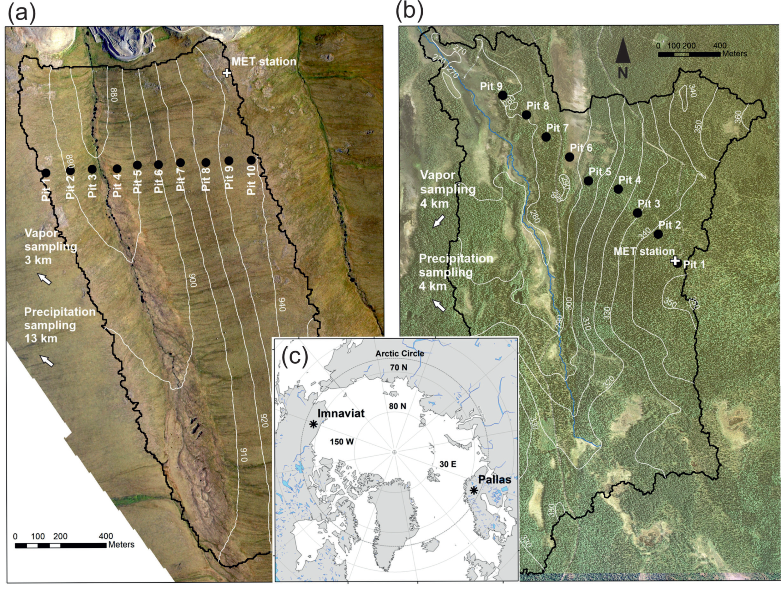
2.1. Study Sites
2.1.1. Imnavait Creek, Alaska, Western Arctic
2.1.2. Pallas, Finnish Lapland, Eastern Arctic
2.2. Snow Sampling and Stable Isotope Analysis
2.2.1. Snowfall
2.2.2. Snowpits
2.2.3. Snow Stable Isotope Analysis
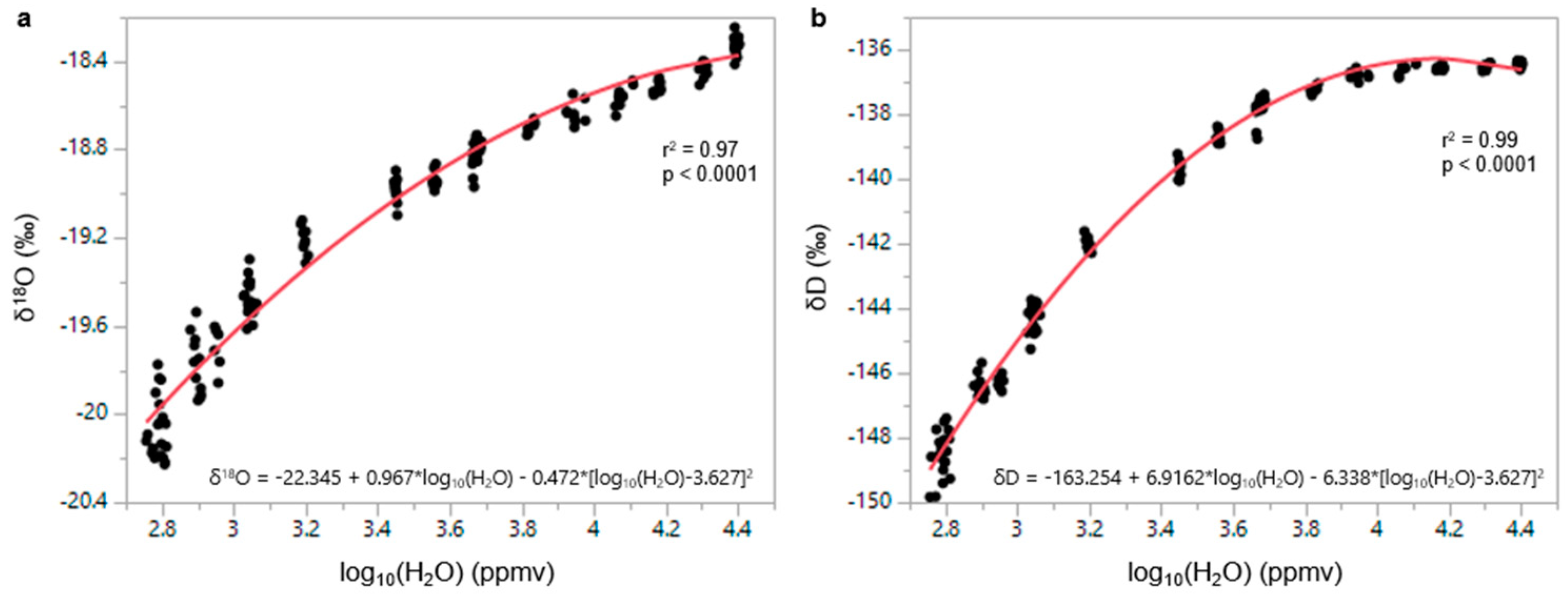
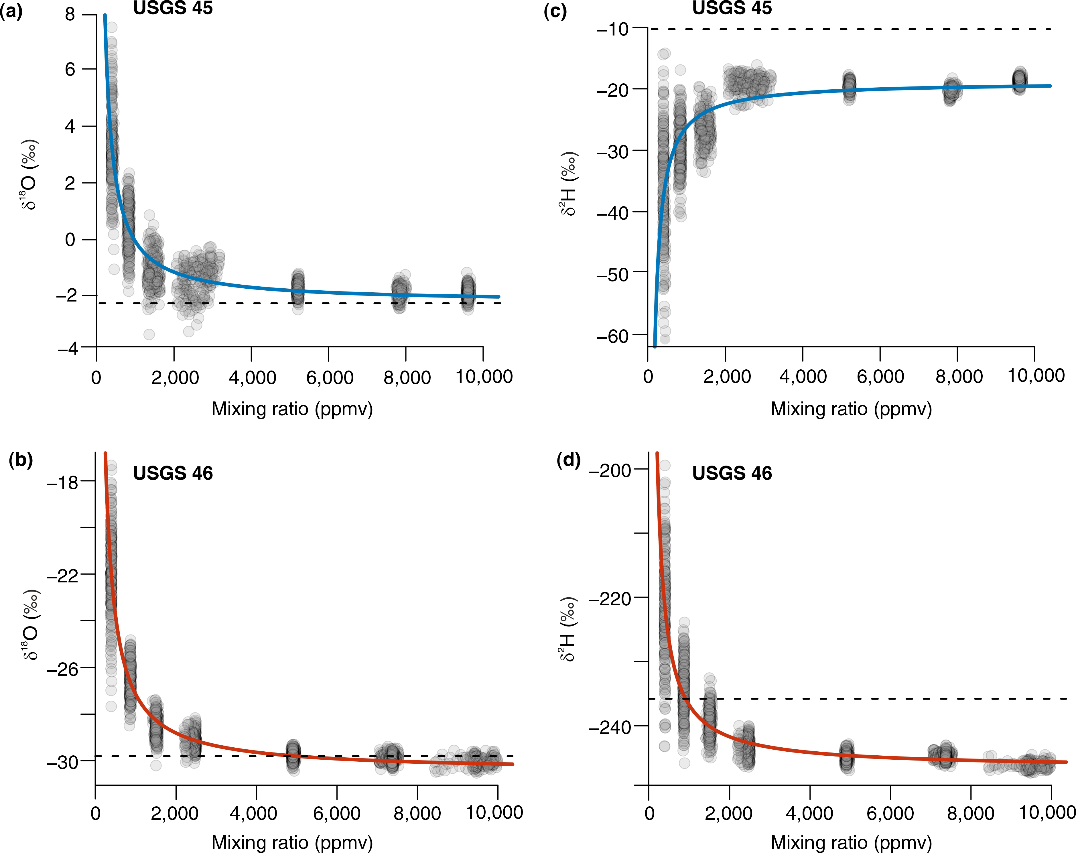
2.3. Atmospheric Water Vapor Analysis
2.4. Synoptic Climatology Analyses
2.5. Data Analysis and Visualization
- ppstart is the y-axis start plotting position in the beginning of the sample i
- ppend is the y-axis end plotting position in the beginning of the sample i
- p is the precipitation amount in sample i (mm)
- n is the number of precipitation events
3. Results
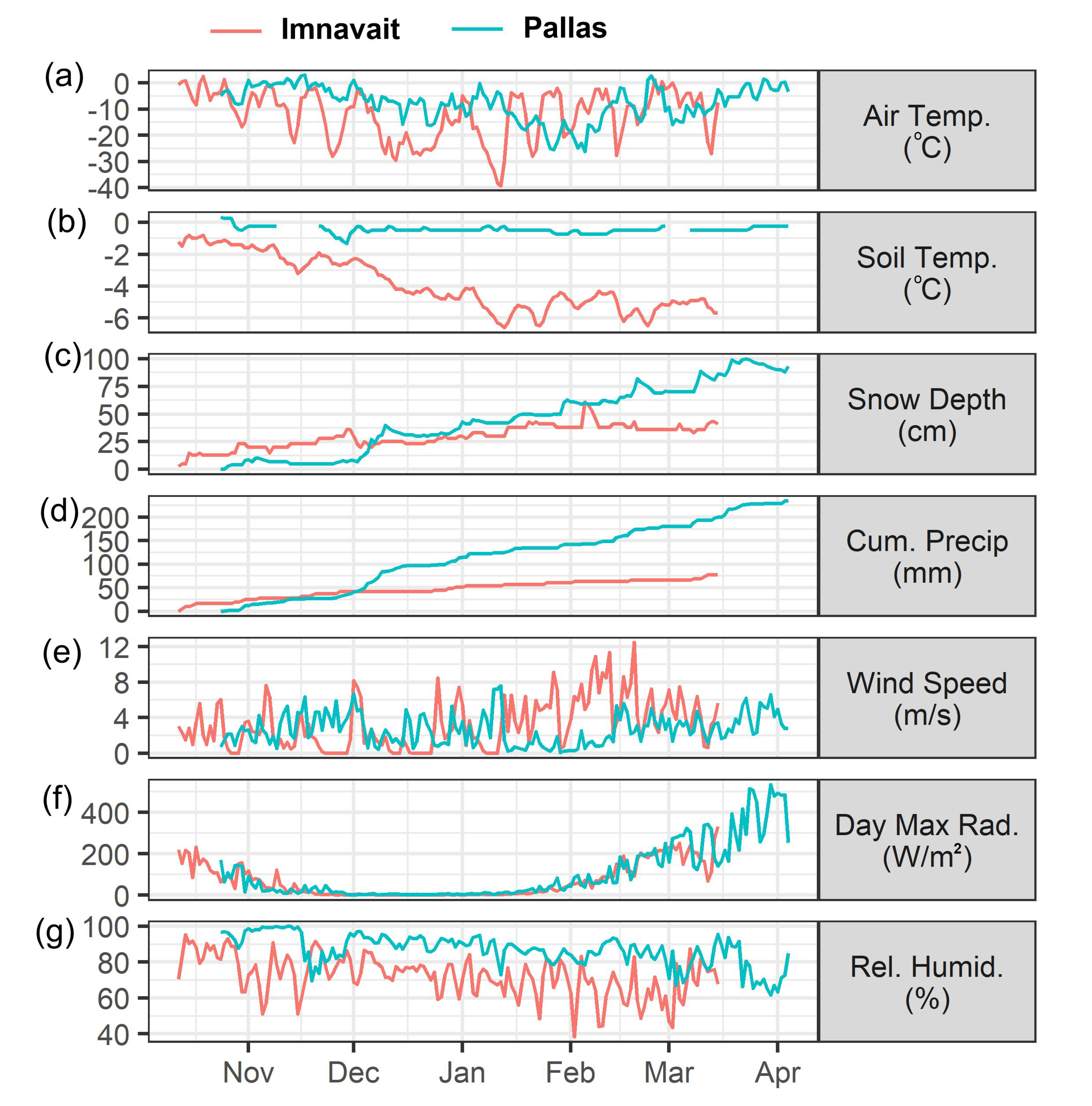
3.1. Climate and Snow Conditions at Imnavait and Pallas
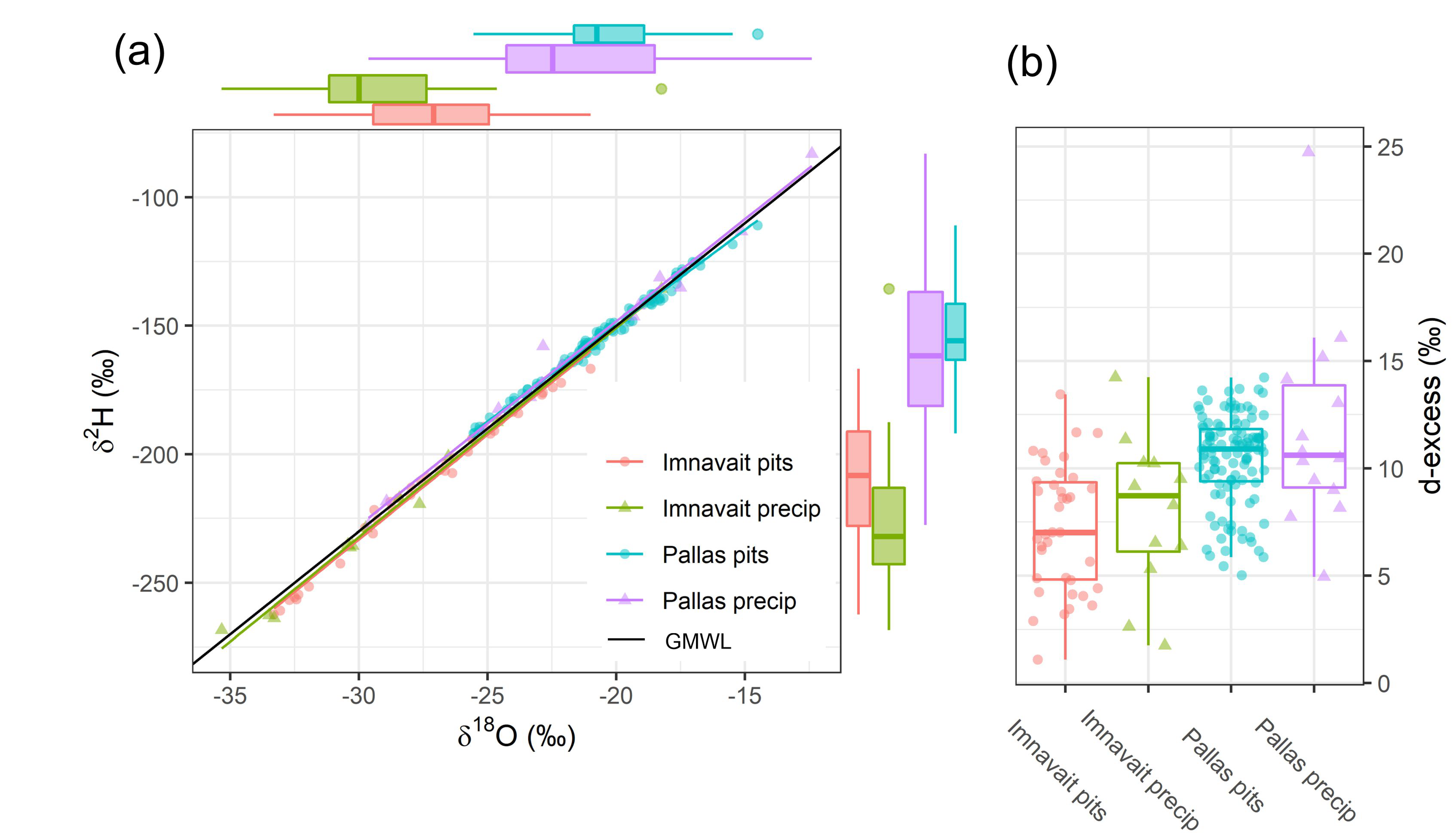
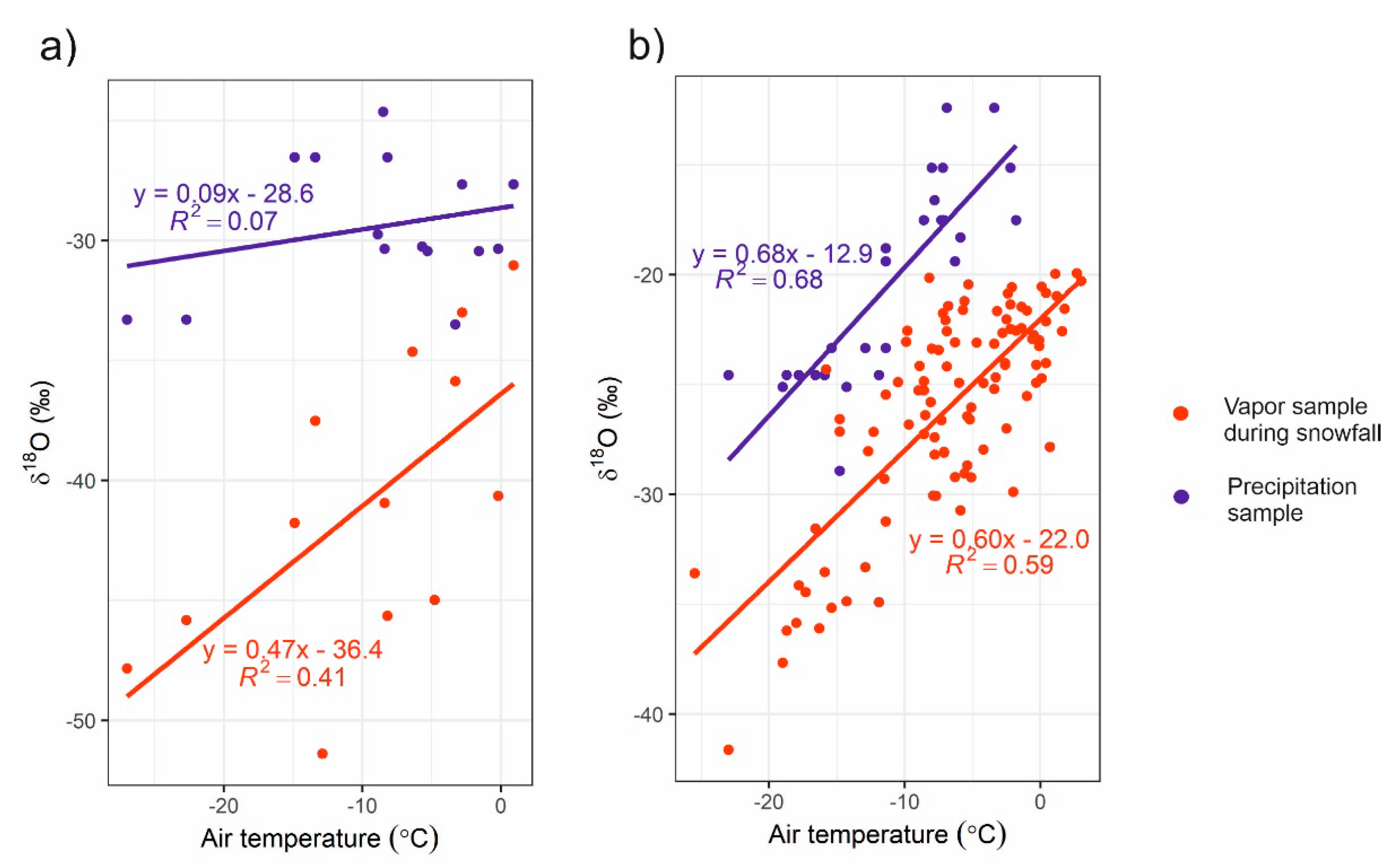
3.2. Isotopic Composition of Snowpack and Precipitation
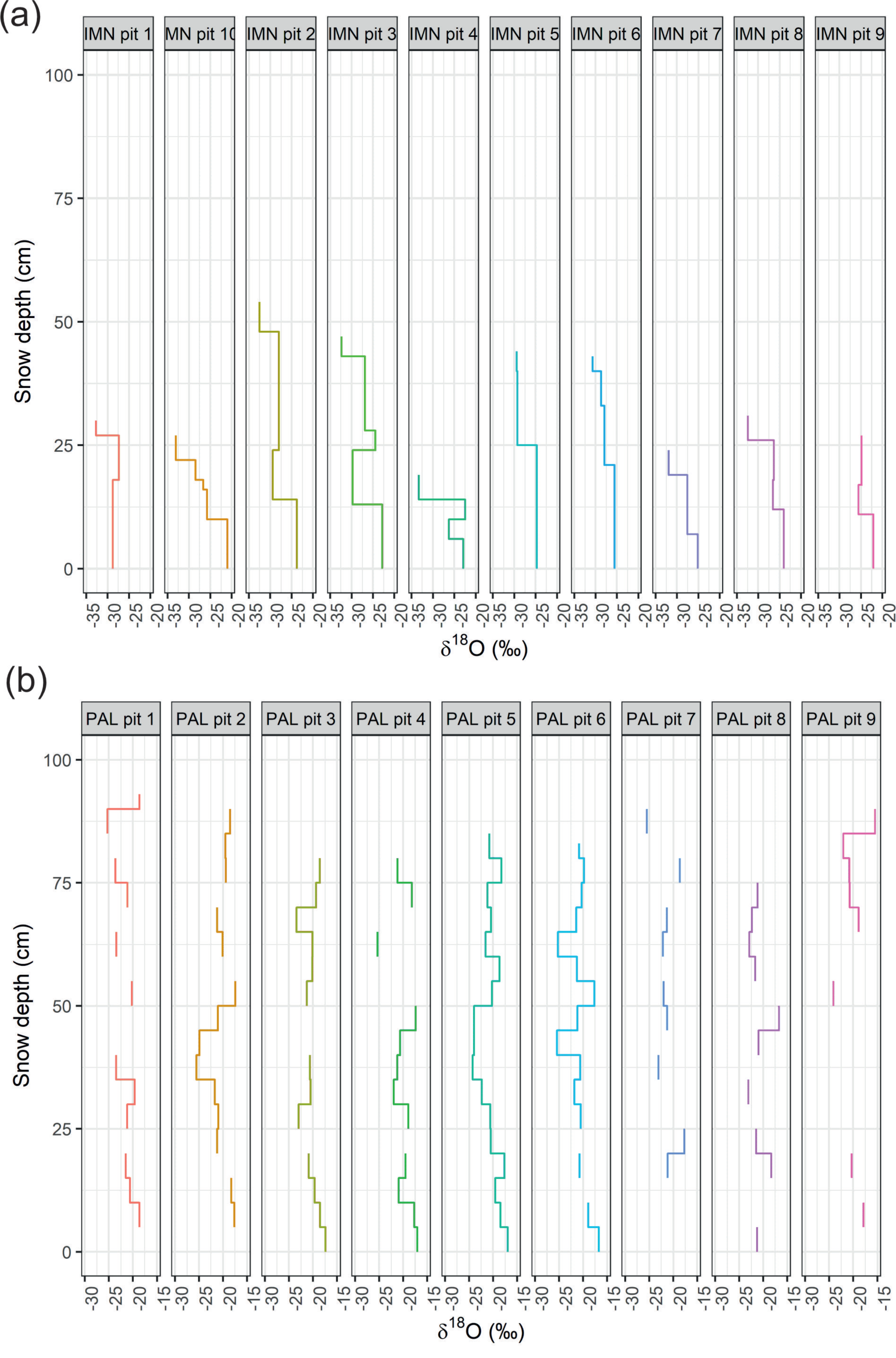
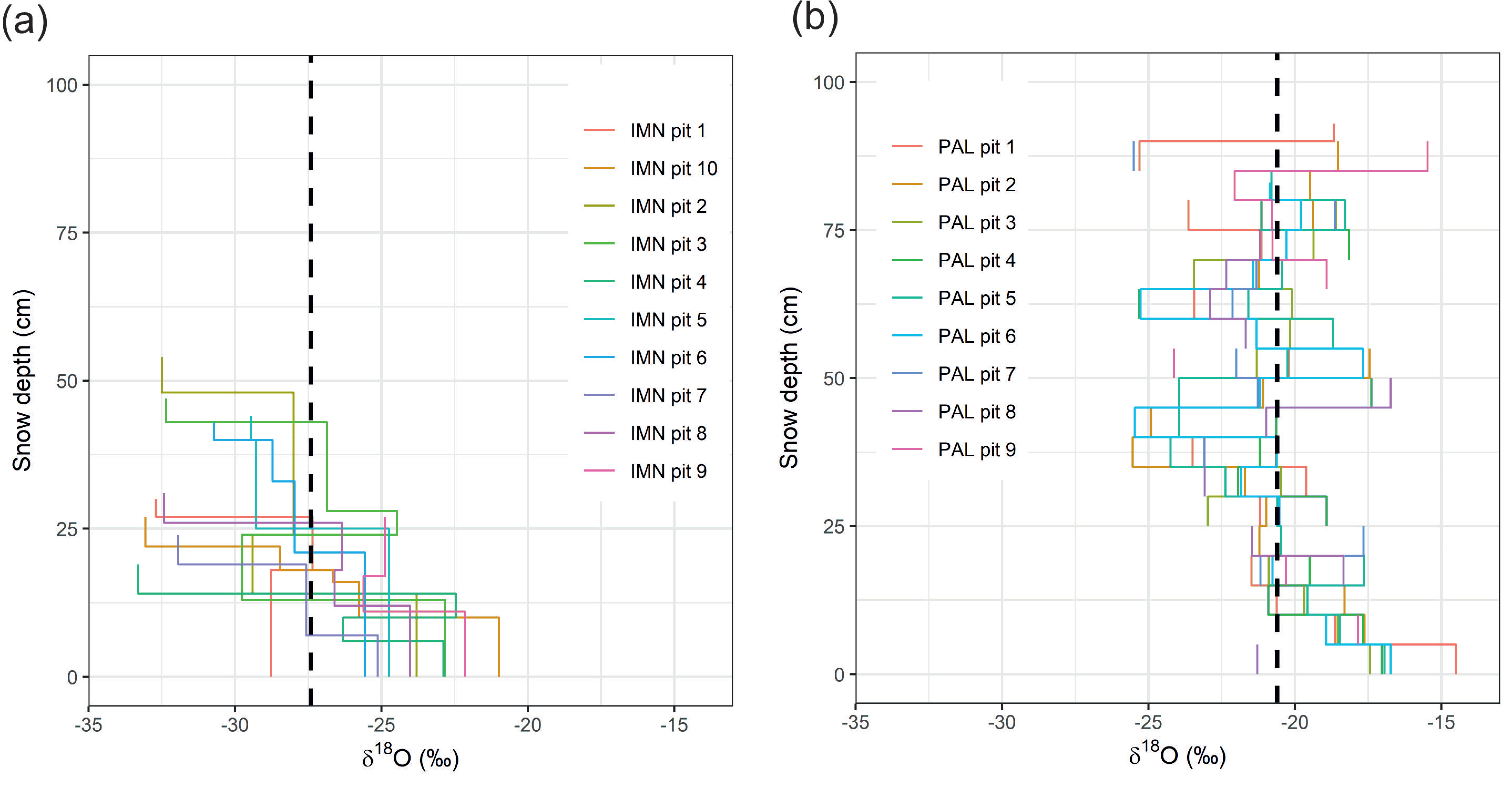
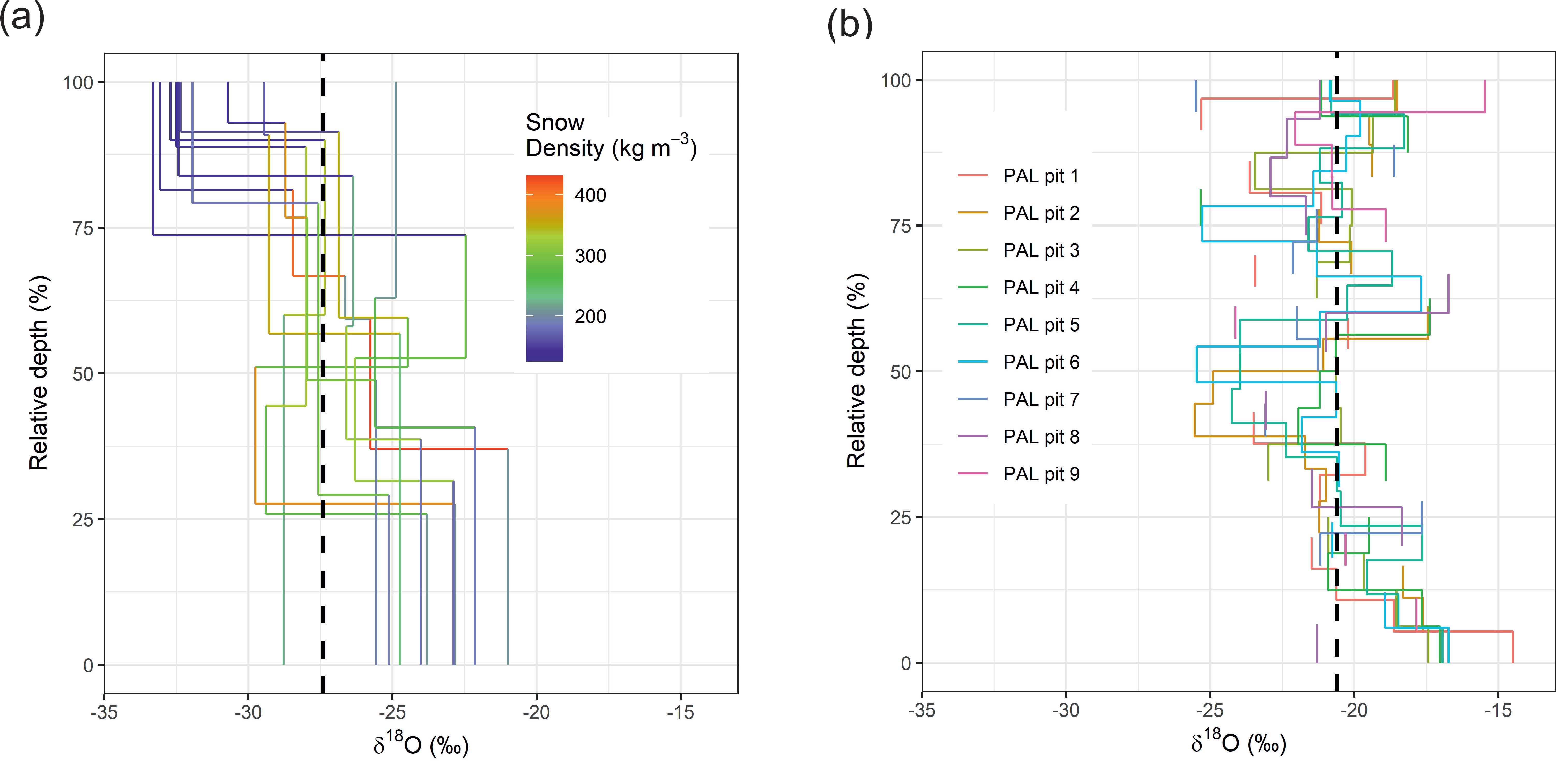
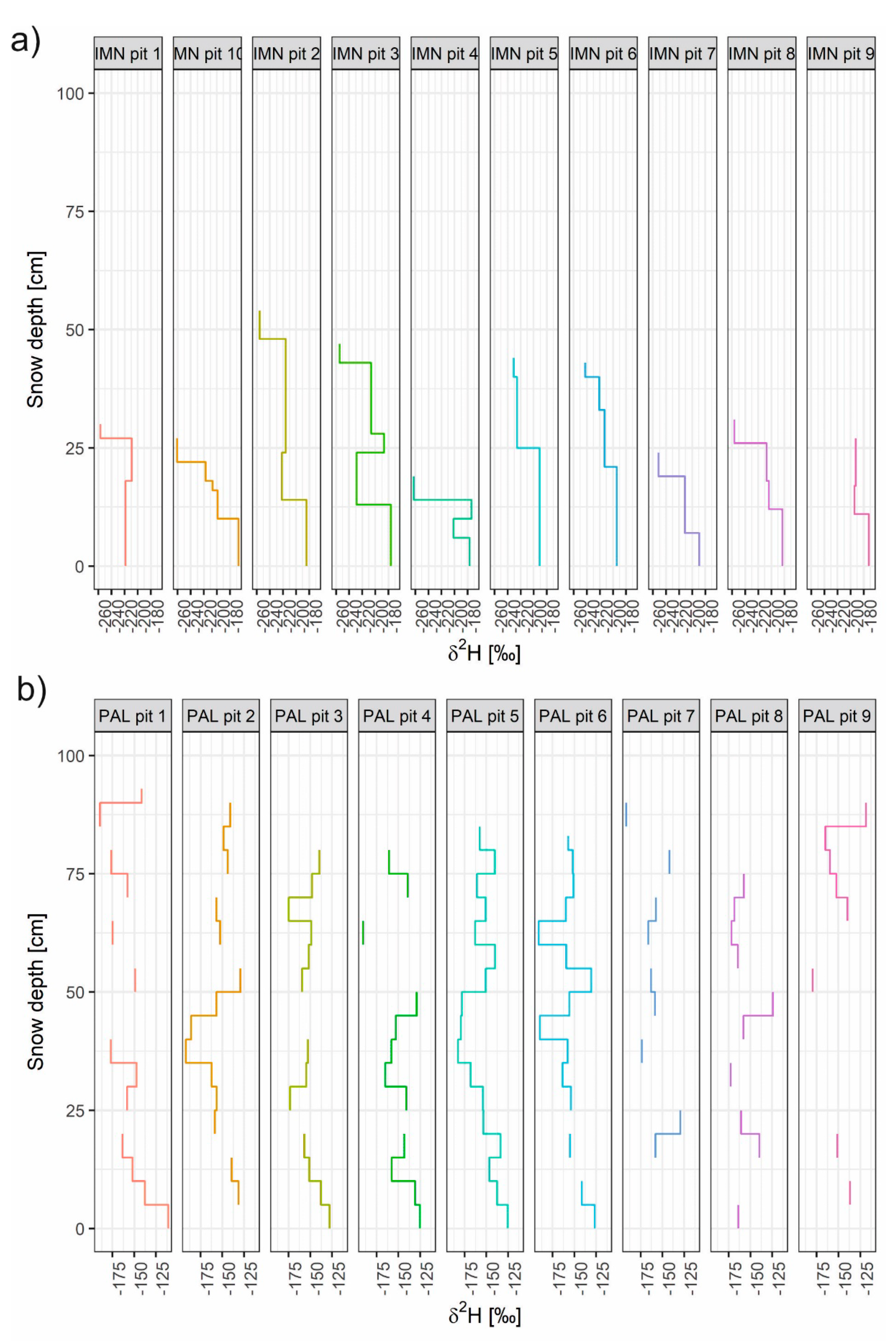
3.3. Isotope Stratigraphy in the Snowpits


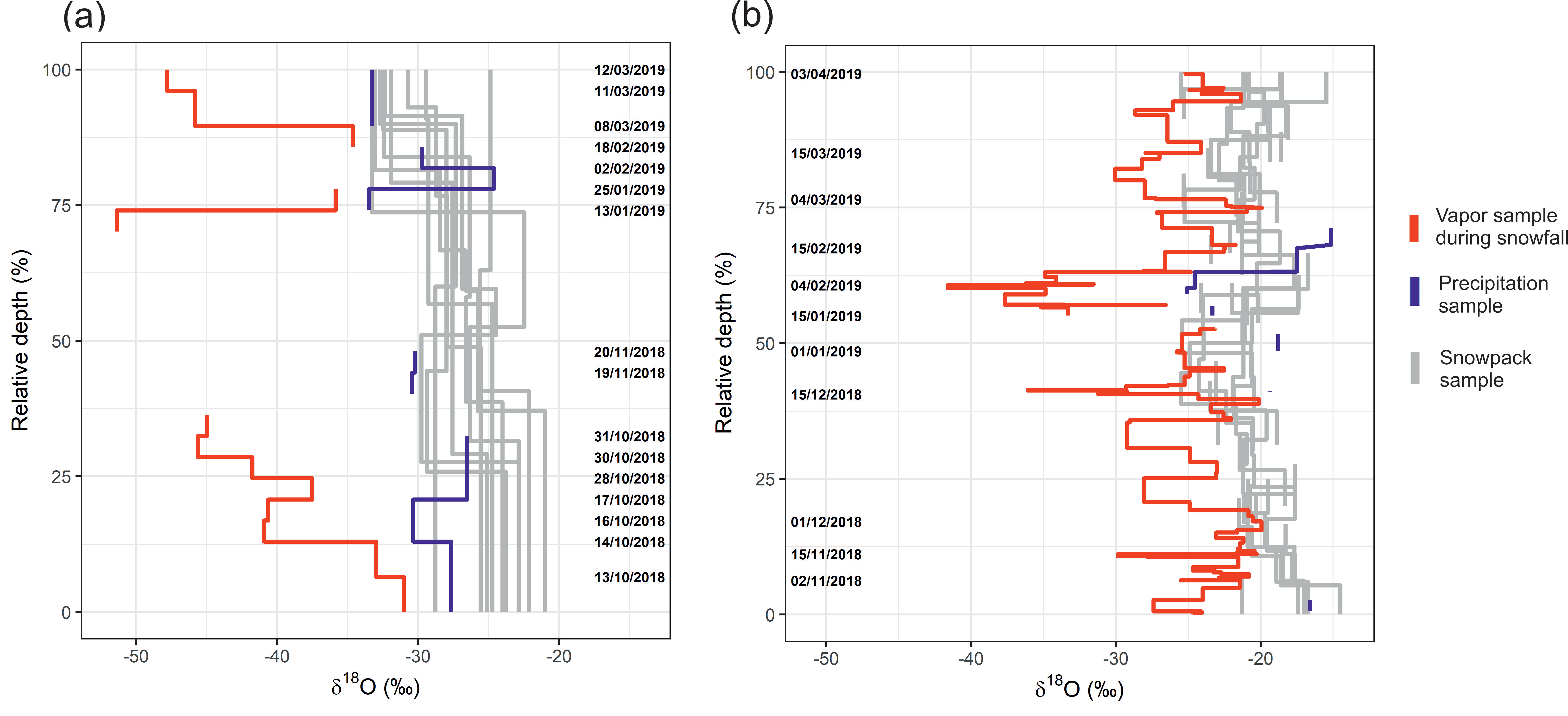
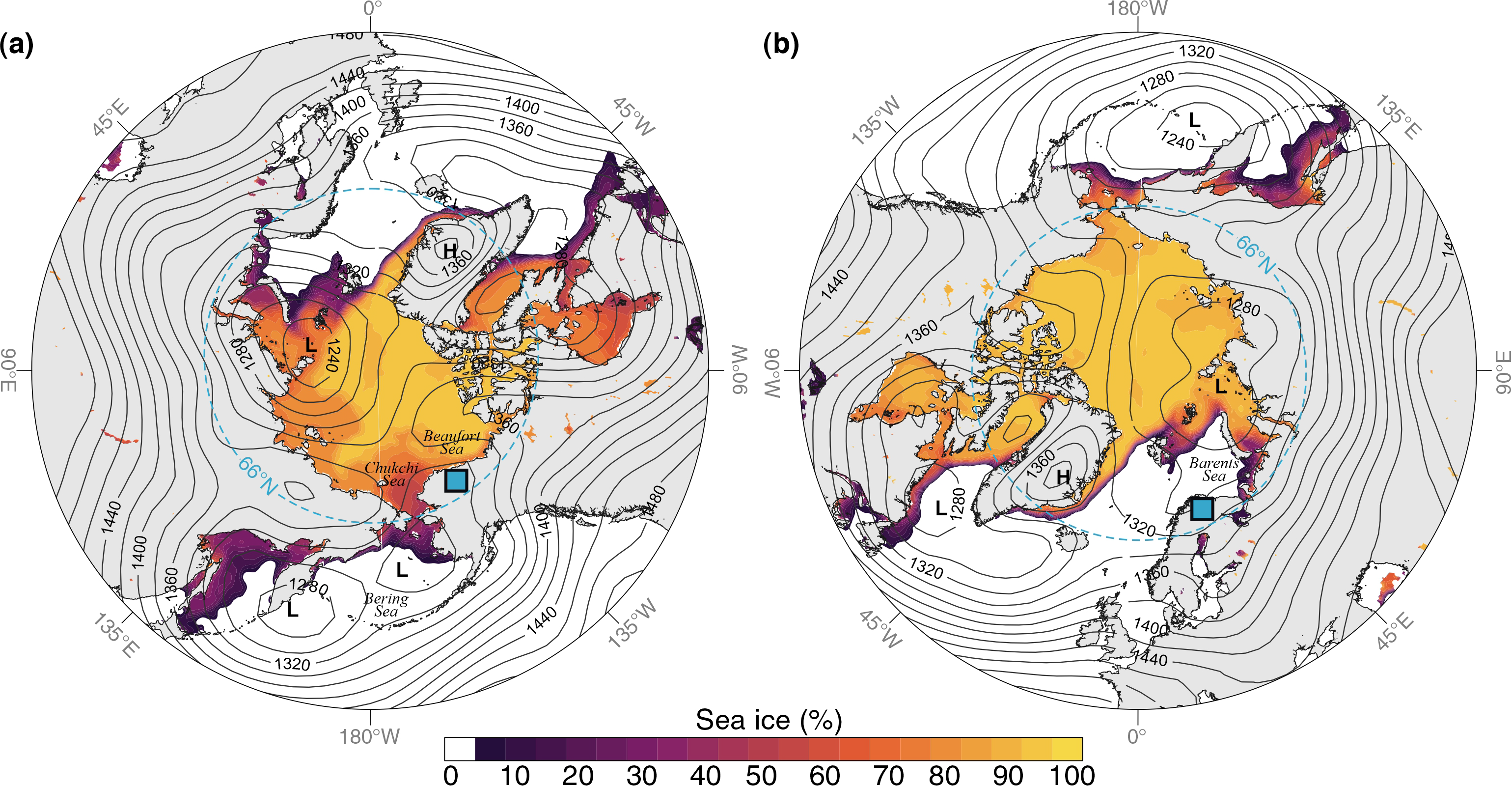
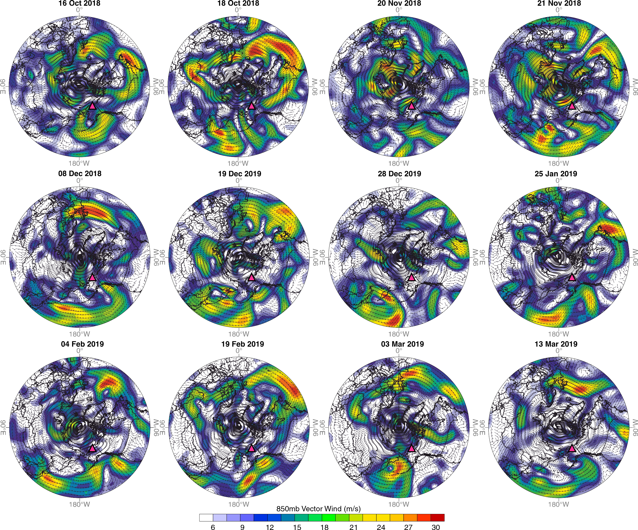
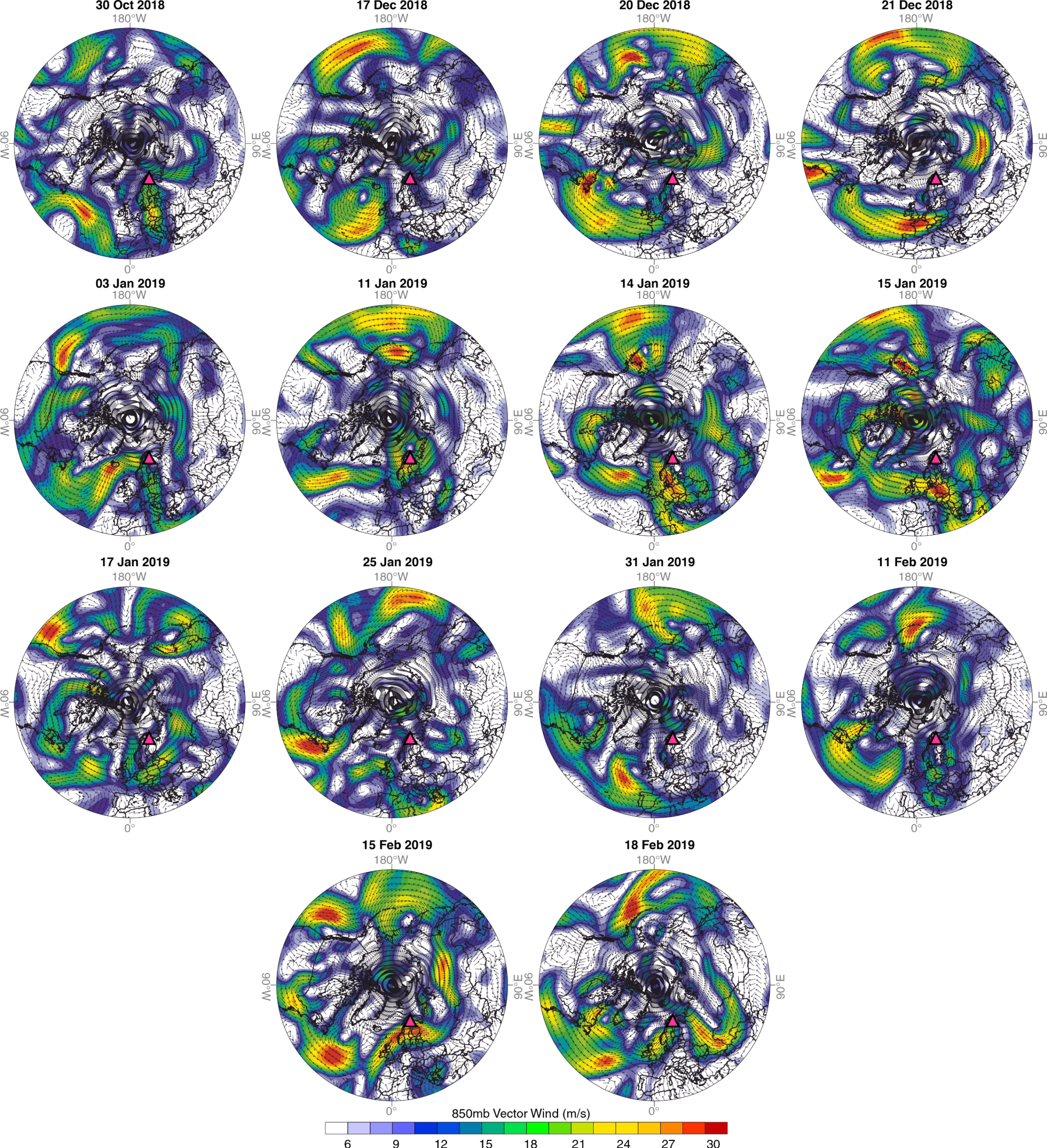
3.4. Synoptic-Scale Moisture Transport and Isotope Hydrology
4. Discussion
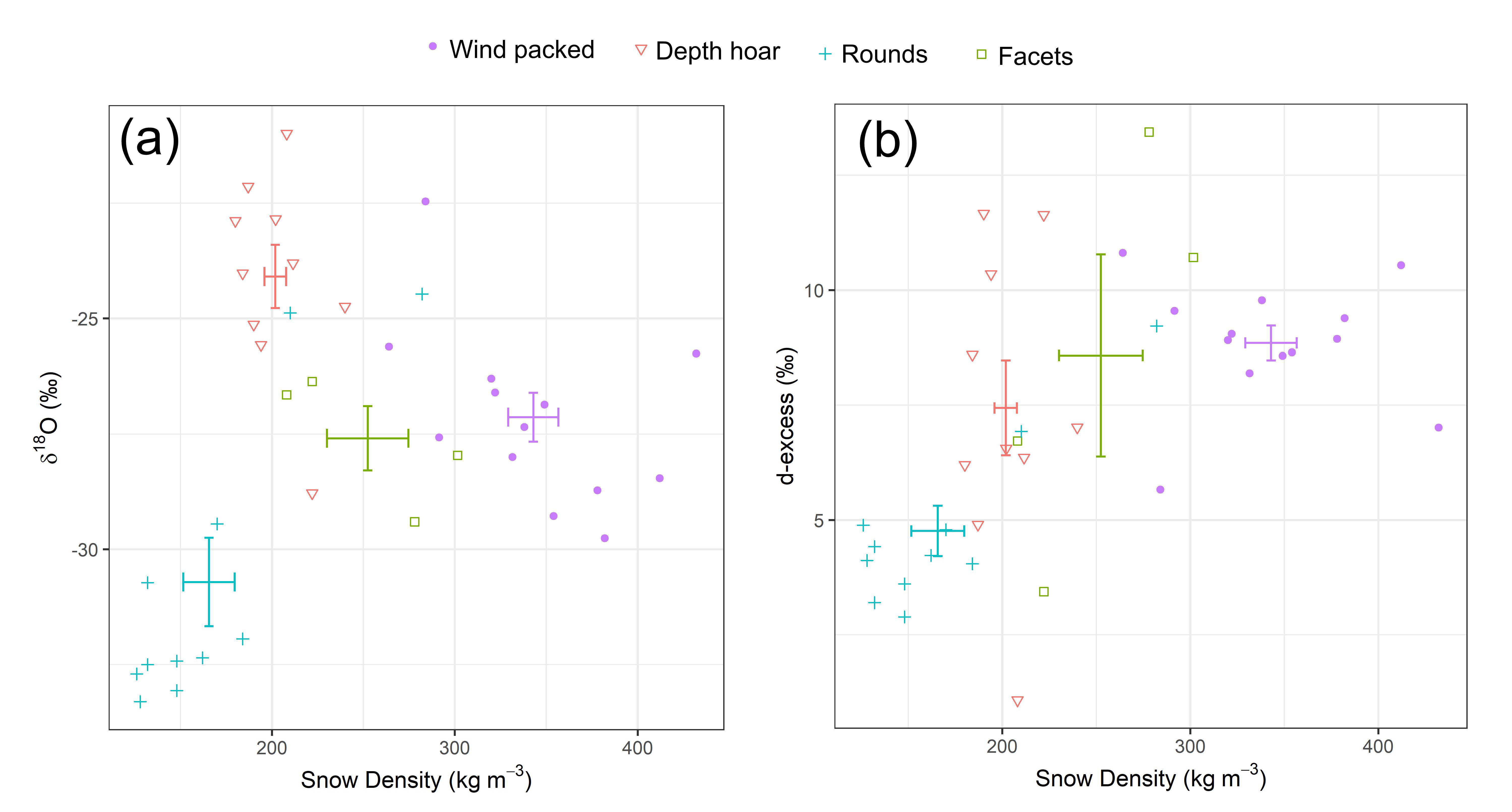
4.1. Isotope Fractionation in the Snowpack
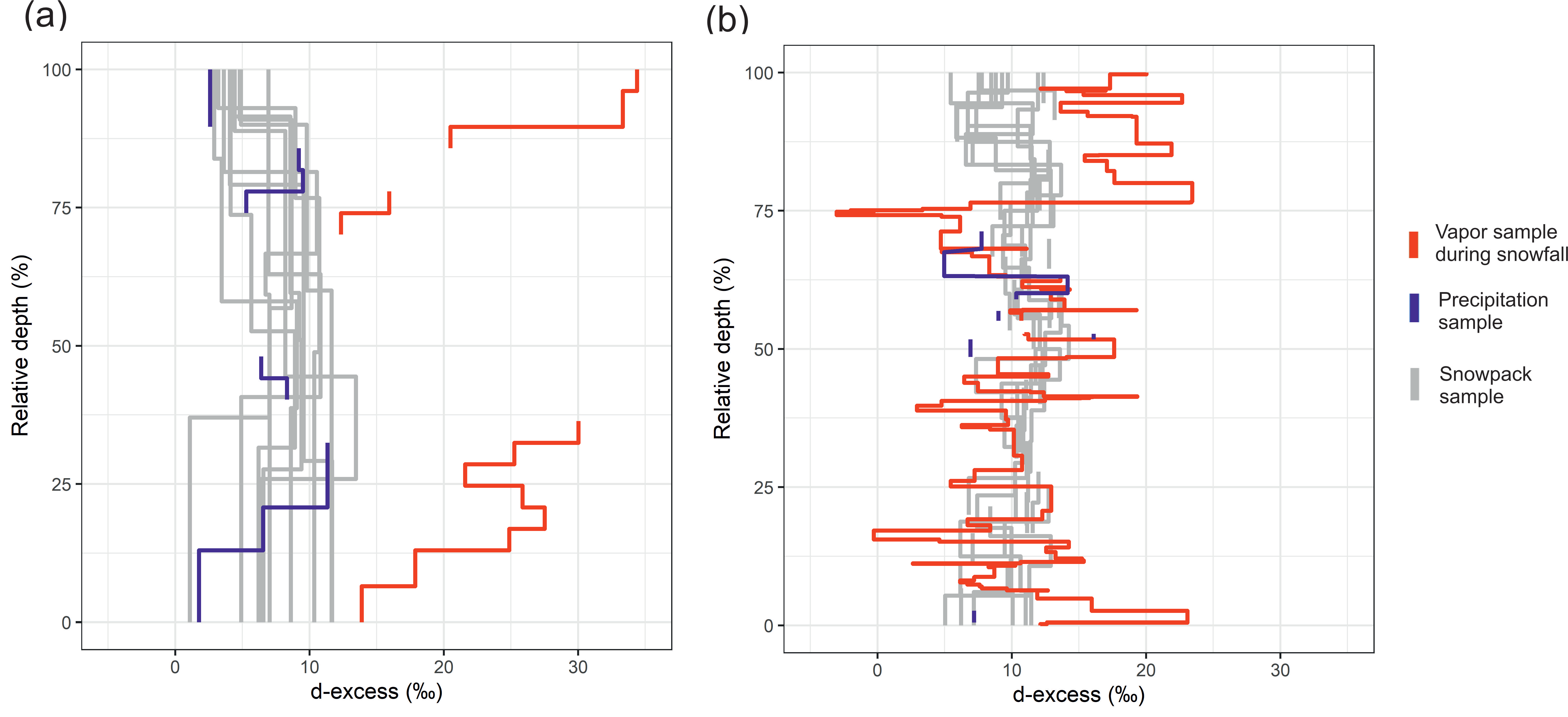
4.2. Contrasting d-excess Values in Snowpack and Vapor between Sites
4.3. Regional Drivers of Snow Amount and Snowpack Isotope Signatures
4.4. Uncertainties and Wider Implications
5. Conclusions
Author Contributions
Funding
Data Availability Statement
Acknowledgments
Conflicts of Interest
Appendix A
Appendix A.1. Imnavait, U.S.A.
Appendix A.2. Pallas, Finland


| Pallas, Finland | Imnavait, USA | ||||||
|---|---|---|---|---|---|---|---|
| Sample Date | δ18O (‰) | δ2H (‰) | d-Excess (‰) | Sample Date | δ18O (‰) | δ2H (‰) | d-Excess (‰) |
| 30 October 2018 | −16.6 | −125.6 | 7.2 | 16 Oct 2018 | −27.6 | −219.4 | 1.8 |
| 17 December 2018 | −19.4 | −145.1 | 10.0 | 18 Oct 2018 | −30.3 | −236.2 | 6.5 |
| 17 December 2018 | −18.9 | −139.3 | 11.5 | 20 Nov 2018 | −30.4 | −235.2 | 8.3 |
| 20 December 2018 | −18.3 | −131.2 | 15.2 | 21 Nov 2018 | −30.3 | −235.6 | 6.4 |
| 21 December 2018 | −22.1 | −165.4 | 11.5 | 08 Dec 2018 | −35.3 | −268.4 | 14.2 |
| 03 January 2019 | −18.8 | −143.4 | 6.9 | 19 Dec 2018 | −28.4 | −217.2 | 10.2 |
| 03 January 2019 | −19.9 | −149.4 | 9.4 | 28 Dec 2018 | −26.5 | −200.9 | 11.3 |
| 11 January 2019 | −12.4 | −83.1 | 16.1 | 25 Jan 2019 | −33.5 | −262.6 | 5.3 |
| 14 January 2019 | −29.6 | −227.6 | 9.4 | 04 Feb 2019 | −24.6 | −187.5 | 9.5 |
| 15 January 2019 | −22.9 | −172.6 | 10.5 | 19 Feb 2019 | −29.7 | −228.7 | 9.2 |
| 17 January 2019 | −23.3 | −177.7 | 9.0 | 03 Mar 2019 | −18.2 | −135.6 | 10.3 |
| 25 January 2019 | −22.8 | −158.0 | 24.7 | 13 Mar 2019 | −33.3 | −263.7 | 2.6 |
| 31 January 2019 | −25.1 | −190.5 | 10.4 | ||||
| 11 February 2019 | −24.6 | −182.4 | 14.1 | ||||
| 15 February 2019 | −17.5 | −135.1 | 5.0 | ||||
| 18 February 2019 | −15.1 | −113.3 | 7.7 | ||||
| Mean: | −20.5 | −152.5 | −11.2 | Mean: | −29.0 | −224.3 | −8.0 |
References
- Overland, J.E.; Hanna, E.; Hanssen-Bauer, I.; Kim, S.J.; Walsh, J.E.; Wang, M.; Bhatt, U.S.; Thoman, R.L.; Ballinger, T.J. Surface Air Temperature. 2020. Available online: https://arctic.noaa.gov/Report-Card/Report-Card-2019/ArtMID/7916/ArticleID/835/Surface-Air-Temperature (accessed on 22 January 2021).
- Bring, A.; Fedorova, I.; Dibike, Y.; Hinzman, L.; Mård, J.; Mernild, S.H.; Prowse, T.; Semenova, O.; Stuefer, S.L.; Woo, M. Arctic Terrestrial Hydrology: A Synthesis of Processes, Regional Effects, and Research Challenges. J. Geophys. Res. Biogeosci. 2016, 121, 621–649. [Google Scholar] [CrossRef]
- Biskaborn, B.K.; Smith, S.L.; Noetzli, J.; Matthes, H.; Vieira, G.; Streletskiy, D.A.; Schoeneich, P.; Romanovsky, V.E.; Lewkowicz, A.G.; Abramov, A.; et al. Permafrost is Warming at a Global Scale. Nat. Commun. 2019, 10, 264. [Google Scholar] [CrossRef] [PubMed]
- Pulliainen, J.; Luojus, K.; Derksen, C.; Mudryk, L.; Lemmetyinen, J.; Salminen, M.; Ikonen, J.; Takala, M.; Cohen, J.; Smolander, T. Patterns and Trends of Northern Hemisphere Snow Mass from 1980 to 2018. Nature 2020, 581, 294–298. [Google Scholar] [CrossRef] [PubMed]
- Klein, E.S.; Welker, J.M. Influence of Sea Ice on Ocean Water Vapor Isotopes and Greenland Ice Core Records. Geophys. Res. Lett. 2016, 43, 12475–12483. [Google Scholar] [CrossRef]
- Stroeve, J.; Notz, D. Changing State of Arctic Sea Ice Across all Seasons. Environ. Res. Lett. 2018, 13, 103001. [Google Scholar] [CrossRef]
- Puntsag, T.; Mitchell, M.J.; Campbell, J.L.; Klein, E.S.; Likens, G.E.; Welker, J.M. Arctic Vortex Changes Alter the Sources and Isotopic Values of Precipitation in Northeastern US. Sci. Rep. 2016, 6, 22647. [Google Scholar] [CrossRef]
- Nygård, T.; Naakka, T.; Vihma, T. Horizontal Moisture Transport Dominates the Regional Moistening Patterns in the Arctic. J. Clim. 2020, 33, 6793–6807. [Google Scholar] [CrossRef]
- Vihma, T.; Screen, J.; Tjernström, M.; Newton, B.; Zhang, X.; Popova, V.; Deser, C.; Holland, M.; Prowse, T. The Atmospheric Role in the Arctic Water Cycle: A Review on Processes, Past and Future Changes, and their Impacts. J. Geophys. Res. Biogeosci. 2016, 121, 586–620. [Google Scholar] [CrossRef]
- Mattingly, K.S.; Mote, T.L.; Fettweis, X. Atmospheric River Impacts on Greenland Ice Sheet Surface Mass Balance. J. Geophys. Res. Atmos. 2018, 123, 8538–8560. [Google Scholar] [CrossRef]
- Nusbaumer, J.; Alexander, P.M.; LeGrande, A.N.; Tedesco, M. Spatial Shift of Greenland Moisture Sources Related to Enhanced Arctic Warming. Geophys. Res. Lett. 2019, 46, 14723–14731. [Google Scholar] [CrossRef]
- Klein, E.S.; Cherry, J.E.; Young, J.; Noone, D.; Leffler, A.J.; Welker, J.M. Arctic Cyclone Water Vapor Isotopes Support Past Sea Ice Retreat Recorded in Greenland Ice. Sci. Rep. 2015, 5, 10295. [Google Scholar] [CrossRef] [PubMed]
- Papritz, L.; Sodemann, H. Characterizing the Local and Intense Water Cycle during a Cold Air Outbreak in the Nordic Seas. Mon. Weather Rev. 2018, 146, 3567–3588. [Google Scholar] [CrossRef]
- Stuefer, S.L.; Kane, D.L.; Dean, K.M. Snow Water Equivalent Measurements in Remote Arctic Alaska Watersheds. Water Resour. Res. 2020, 56, e2019WR025621. [Google Scholar] [CrossRef]
- Faranda, D. An Attempt to Explain Recent Changes in European Snowfall Extremes. Weather Clim. Dyn. 2020, 1, 445–458. [Google Scholar] [CrossRef]
- Lawrence, Z.D.; Perlwitz, J.; Butler, A.H.; Manney, G.L.; Newman, P.A.; Lee, S.H.; Nash, E.R. The Remarkably Strong Arctic Stratospheric Polar Vortex of Winter 2020: Links to Record-Breaking Arctic Oscillation and Ozone Loss. J. Geophys. Res. Atmos. 2020, 125, e2020JD033271. [Google Scholar] [CrossRef]
- Marks, D.; Dozier, J. Climate and Energy Exchange at the Snow Surface in the Alpine Region of the Sierra Nevada: 2. Snow Cover Energy Balance. Water Resour. Res. 1992, 28, 3043–3054. [Google Scholar] [CrossRef]
- Groisman, P.Y.; Karl, T.R.; Knight, R.W. Observed Impact of Snow Cover on the Heat Balance and the Rise of Continental Spring Temperatures. Science 1994, 263, 198–200. [Google Scholar] [CrossRef]
- Stiegler, C.; Lund, M.; Christensen, T.R.; Mastepanov, M.; Lindroth, A. Two Years with Extreme and Little Snowfall: Effects on Energy Partitioning and Surface Energy Exchange in a High-Arctic Tundra Ecosystem. Cryosphere 2016, 10, 1395–1413. [Google Scholar] [CrossRef]
- Allen, S.T.; Kirchner, J.W.; Braun, S.; Siegwolf, R.T.; Goldsmith, G.R. Seasonal Origins of Soil Water used by Trees. Hydrol. Earth Syst. Sci. 2019, 23, 1199–1210. [Google Scholar] [CrossRef]
- Kirchner, J.W.; Allen, S.T. Seasonal Partitioning of Precipitation between Streamflow and Evapotranspiration, Inferred from End-Member Splitting Analysis. In Proceedings of the AGU Fall Meeting, San Francisco, CA, USA, 9–13 December 2019. [Google Scholar]
- Meriö, L.; Ala-aho, P.; Linjama, J.; Hjort, J.; Kløve, B.; Marttila, H. Snow to Precipitation Ratio Controls Catchment Storage and Summer Flows in Boreal Headwater Catchments. Water Resour. Res. 2019, 55, 4096–4109. [Google Scholar] [CrossRef]
- Tetzlaff, D.; Buttle, J.; Carey, S.K.; McGuire, K.; Laudon, H.; Soulsby, C. Tracer-based Assessment of Flow Paths, Storage and Runoff Generation in Northern Catchments: A Review. Hydrol. Process. 2015, 29, 3475–3490. [Google Scholar] [CrossRef]
- Bokhorst, S.; Pedersen, S.H.; Brucker, L.; Anisimov, O.; Bjerke, J.W.; Brown, R.D.; Ehrich, D.; Essery, R.L.; Heilig, A.; Ingvander, S. Changing Arctic Snow Cover: A Review of Recent Developments and Assessment of Future Needs for Observations, Modelling, and Impacts. Ambio 2016, 45, 516–537. [Google Scholar] [CrossRef] [PubMed]
- Callaghan, T.V.; Johansson, M.; Brown, R.D.; Groisman, P.Y.; Labba, N.; Radionov, V.; Bradley, R.S.; Blangy, S.; Bulygina, O.N.; Christensen, T.R. Multiple Effects of Changes in Arctic Snow Cover. Ambio 2011, 40, 32–45. [Google Scholar] [CrossRef]
- Blanc-Betes, E.; Welker, J.M.; Sturchio, N.C.; Chanton, J.P.; Gonzalez-Meler, M.A. Winter Precipitation and Snow Accumulation Drive the Methane Sink Or Source Strength of Arctic Tussock Tundra. Glob. Chang. Biol. 2016, 22, 2818–2833. [Google Scholar] [CrossRef]
- Lupascu, M.; Czimczik, C.I.; Welker, M.C.; Ziolkowski, L.A.; Cooper, E.J.; Welker, J.M. Winter Ecosystem Respiration and Sources of CO2 from the High Arctic Tundra of Svalbard: Response to a Deeper Snow Experiment. J. Geophys. Res. Biogeosci. 2018, 123, 2627–2642. [Google Scholar] [CrossRef]
- Natali, S.M.; Watts, J.D.; Rogers, B.M.; Potter, S.; Ludwig, S.M.; Selbmann, A.; Sullivan, P.F.; Abbott, B.W.; Arndt, K.A.; Birch, L. Large Loss of CO 2 in Winter Observed Across the Northern Permafrost Region. Nat. Clim. Chang. 2019, 9, 852–857. [Google Scholar] [CrossRef]
- Sturm, M.; Schimel, J.; Michaelson, G.; Welker, J.M.; Oberbauer, S.F.; Liston, G.E.; Fahnestock, J.; Romanovsky, V.E. Winter Biological Processes could Help Convert Arctic Tundra to Shrubland. Bioscience 2005, 55, 17–26. [Google Scholar] [CrossRef]
- Jespersen, R.G.; Leffler, A.J.; Oberbauer, S.F.; Welker, J.M. Arctic Plant Ecophysiology and Water Source Utilization in Response to Altered Snow: Isotopic (Δ 18 O and Δ 2 H) Evidence for Meltwater Subsidies to Deciduous Shrubs. Oecologia 2018, 187, 1009–1023. [Google Scholar] [CrossRef]
- Welker, J.M.; Rayback, S.; Henry, G.H. Arctic and North Atlantic Oscillation Phase Changes are Recorded in the Isotopes (δ18O and δ13C) of Cassiope Tetragona Plants. Glob. Chang. Biol. 2005, 11, 997–1002. [Google Scholar] [CrossRef]
- Welker, J.M.; THE Heaton; Spiro, B.; Callaghan, T.V. Indirect Effects of Winter Climate on the D13C and the DD Characteristics of Annual Growth Segments in the Long-Lived Arctic Plant Cassiope Tetragona: A Preliminary Analysis. Paleoclimatological Res. 1995, 15, 105–120. [Google Scholar]
- Hansen, B.B.; Lorentzen, J.R.; Welker, J.M.; Varpe, Ø.; Aanes, R.; Beumer, L.T.; Pedersen, Å.Ø. Reindeer Turning Maritime: Ice-locked Tundra Triggers Changes in Dietary Niche Utilization. Ecosphere 2019, 10, e02672. [Google Scholar] [CrossRef]
- Bowen, G.J.; Cai, Z.; Fiorella, R.P.; Putman, A.L. Isotopes in the Water Cycle: Regional-to Global-Scale Patterns and Applications. Annu. Rev. Earth Planet. Sci. 2019, 47, 453–479. [Google Scholar] [CrossRef]
- Vachon, R.W.; Welker, J.M.; White, J.; Vaughn, B.H. Monthly Precipitation Isoscapes (δ18O) of the United States: Connections with Surface Temperatures, Moisture Source Conditions, and Air Mass Trajectories. J. Geophys. Res. Atmos. 2010, 115, 115. [Google Scholar] [CrossRef]
- Akers, P.D.; Welker, J.M.; Brook, G.A. Reassessing the Role of Temperature in Precipitation Oxygen Isotopes Across the Eastern and Central U Nited S Tates through Weekly Precipitation-day Data. Water Resour. Res. 2017, 53, 7644–7661. [Google Scholar] [CrossRef]
- Sjostrom, D.J.; Welker, J.M. The Influence of Air Mass Source on the Seasonal Isotopic Composition of Precipitation, Eastern USA. J. Geochem. Explor. 2009, 102, 103–112. [Google Scholar] [CrossRef]
- Bailey, H.L.; Kaufman, D.S.; Henderson, A.C.; Leng, M.J. Synoptic Scale Controls on the δ18O in Precipitation Across Beringia. Geophys. Res. Lett. 2015, 42, 4608–4616. [Google Scholar] [CrossRef]
- Sprenger, M.; Leistert, H.; Gimbel, K.; Weiler, M. Illuminating Hydrological Processes at the Soil-vegetation-atmosphere Interface with Water Stable Isotopes. Rev. Geophys. 2016, 54, 674–704. [Google Scholar] [CrossRef]
- Penna, D.; Hopp, L.; Scandellari, F.; Allen, S.T.; Benettin, P.; Beyer, M.; Dawson17, J.W. Tracing Ecosystem Water Fluxes using Hydrogen and Oxygen Stable Isotopes: Challenges and Opportunities from an Interdisciplinary Perspective. Biogeosci. Discuss. 2018, 15, 6399–6415. [Google Scholar] [CrossRef]
- Welker, J.M.; Fahnestock, J.T.; Sullivan, P.F.; Chimner, R.A. Leaf Mineral Nutrition of Arctic Plants in Response to Warming and Deeper Snow in Northern Alaska. Oikos 2005, 109, 167–177. [Google Scholar] [CrossRef]
- Welker, J.M. Isotopic (δ18O) Characteristics of Weekly Precipitation Collected Across the USA: An Initial Analysis with Application to Water Source Studies. Hydrol. Process. 2000, 14, 1449–1464. [Google Scholar] [CrossRef]
- Bailey, H.L.; Klein, E.S.; Welker, J.M. Synoptic and Mesoscale Mechanisms Drive Winter Precipitation δ18O/δ2H in South-central Alaska. J. Geophys. Res. Atmos. 2019, 124, 4252–4266. [Google Scholar] [CrossRef]
- Kopec, B.G.; Feng, X.; Michel, F.A.; Posmentier, E.S. Influence of Sea Ice on Arctic Precipitation. Proc. Natl. Acad. Sci. USA 2016, 113, 46–51. [Google Scholar] [CrossRef] [PubMed]
- Charles, C.D.; Rind, D.V.; Jouzel, J.; Koster, R.D.; Fairbanks, R.G. Glacial-Interglacial Changes in Moisture Sources for Greenland: Influences on the Ice Core Record of Climate. Science 1994, 263, 508–511. [Google Scholar] [CrossRef] [PubMed]
- Daniels, W.C.; Russell, J.M.; Giblin, A.E.; Welker, J.M.; Klein, E.S.; Huang, Y. Hydrogen Isotope Fractionation in Leaf Waxes in the Alaskan Arctic Tundra. Geochim. Cosmochim. Acta 2017, 213, 216–236. [Google Scholar]
- Sinclair, K.E.; Marshall, S.J. Post-Depositional Modification of Stable Water Isotopes in Winter Snowpacks in the Canadian Rocky Mountains. Ann. Glaciol. 2008, 49, 96–106. [Google Scholar] [CrossRef][Green Version]
- Helsen, M.M.; Van de Wal, R.; Van den Broeke, M.R.; Masson-Delmotte, V.; Meijer, H.; Scheele, M.P.; Werner, M. Modeling the Isotopic Composition of Antarctic Snow using Backward Trajectories: Simulation of Snow Pit Records. J. Geophys. Res. Atmos. 2006, 111, 111. [Google Scholar]
- Grootes, P.M.; Stuiver, M. Oxygen 18/16 Variability in Greenland Snow and Ice with 10− 3-to 105-year Time Resolution. J. Geophys. Res. Ocean. 1997, 102, 26455–26470. [Google Scholar]
- Steen-Larsen, H.C.; Masson-Delmotte, V.; Sjolte, J.; Johnsen, S.J.; Vinther, B.M.; Bréon, F.; Clausen, H.B.; Dahl-Jensen, D.; Falourd, S.; Fettweis, X. Understanding the Climatic Signal in the Water Stable Isotope Records from the NEEM Shallow Firn/Ice Cores in Northwest Greenland. J. Geophys. Res. Atmos. 2011, 116. [Google Scholar] [CrossRef]
- Lechler, A.R.; Niemi, N.A. The Influence of Snow Sublimation on the Isotopic Composition of Spring and Surface Waters in the Southwestern United States: Implications for Stable Isotope–based Paleoaltimetry and Hydrologic Studies. Bulletin 2012, 124, 318–334. [Google Scholar] [CrossRef]
- Earman, S.; Campbell, A.R.; Phillips, F.M.; Newman, B.D. Isotopic Exchange between Snow and Atmospheric Water Vapor: Estimation of the Snowmelt Component of Groundwater Recharge in the Southwestern United States. J. Geophys. Res. Atmos. 2006, 111, 111. [Google Scholar] [CrossRef]
- Ala-aho, P.; Tetzlaff, D.; McNamara, J.P.; Laudon, H.; Kormos, P.; Soulsby, C. Modeling the Isotopic Evolution of Snowpack and Snowmelt: Testing a Spatially Distributed Parsimonious Approach. Water Resour. Res. 2017, 53, 5813–5830. [Google Scholar] [CrossRef] [PubMed]
- Madsen, M.V.; Steen-Larsen, H.C.; Hörhold, M.; Box, J.; Berben, S.M.P.; Capron, E.; Faber, A.; Hubbard, A.; Jensen, M.F.; Jones, T.R. Evidence of Isotopic Fractionation during Vapor Exchange between the Atmosphere and the Snow Surface in Greenland. J. Geophys. Res. Atmos. 2019, 124, 2932–2945. [Google Scholar] [CrossRef] [PubMed]
- Kopec, B.G.; Akers, P.D.; Klein, E.S.; Welker, J.M. Significant Water Vapor Fluxes from the Greenland Ice Sheet Detected through Water Vapor Isotopic (δ18O, δD, Deuterium Excess) Measurements. Cryosphere Discuss 2020. under review. [Google Scholar]
- Sturm, M.; Benson, C.S. Vapor Transport, Grain Growth and Depth-Hoar Development in the Subarctic Snow. J. Glaciol. 1997, 43, 42–59. [Google Scholar] [CrossRef]
- Neumann, T.A.; Albert, M.R.; Lomonaco, R.; Engel, C.; Courville, Z.; Perron, F. Experimental Determination of Snow Sublimation Rate and Stable-Isotopic Exchange. Ann. Glaciol. 2008, 49, 1–6. [Google Scholar] [CrossRef]
- Friedman, I.; Benson, C.; Gleason, J. Isotopic Changes during Snow Metamorphism. In Stable Isotope Geochemistry: A Tribute to Samuel Epstein; The Geochemical Society: San Antonio, TX, USA, 1991; pp. 211–221. [Google Scholar]
- Von Freyberg, J.; Bjarnadóttir, T.R.; Allen, S.T. Influences of Forest Canopy on Snowpack Accumulation and Isotope Ratios. Hydrol. Process. 2020, 34, 679–690. [Google Scholar] [CrossRef]
- Koeniger, P.; Hubbart, J.A.; Link, T.; Marshall, J.D. Isotopic Variation of Snow Cover and Streamflow in Response to Changes in Canopy Structure in a Snow-dominated Mountain Catchment. Hydrol. Process. Int. J. 2008, 22, 557–566. [Google Scholar] [CrossRef]
- Moser, H.; Stichler, W. Deuterium and Oxygen-18 Contents as an Index of the Properties of Snow Covers. Int. Assoc. Hydrol. Sci. Publ. 1974, 114, 122–135. [Google Scholar]
- Evans, S.L.; Flores, A.N.; Heilig, A.; Kohn, M.J.; Marshall, H.; McNamara, J.P. Isotopic Evidence for Lateral Flow and Diffusive Transport, but Not Sublimation, in a Sloped Seasonal Snowpack, Idaho, USA. Geophys. Res. Lett. 2016, 43, 3298–3306. [Google Scholar] [CrossRef]
- Unnikrishna, P.V.; McDonnell, J.J.; Kendall, C. Isotope Variations in a Sierra Nevada Snowpack and their Relation to Meltwater. J. Hydrol. 2002, 260, 38–57. [Google Scholar] [CrossRef]
- Beria, H.; Larsen, J.R.; Ceperley, N.C.; Michelon, A.; Vennemann, T.; Schaefli, B. Understanding Snow Hydrological Processes through the Lens of Stable Water Isotopes. Wiley Interdiscip. Rev. Water 2018, 5, e1311. [Google Scholar] [CrossRef]
- Pu, T.; Wang, K.; Kong, Y.; Shi, X.; Kang, S.; Huang, Y.; He, Y.; Wang, S.; Lee, J.; Cuntz, M. Observing and Modeling the Isotopic Evolution of Snow Meltwater on the Southeastern Tibetan Plateau. Water Resour. Res. 2020, 56, e2019WR026423. [Google Scholar] [CrossRef]
- Taylor, S.; Feng, X.; Kirchner, J.W.; Osterhuber, R.; Klaue, B.; Renshaw, C.E. Isotopic Evolution of a Seasonal Snowpack and its Melt. Water Resour. Res. 2001, 37, 759–769. [Google Scholar] [CrossRef]
- Ham, J.; Do Hur, S.; Lee, W.S.; Han, Y.; Jung, H.; Lee, J. Isotopic Variations of Meltwater from Ice by Isotopic Exchange between Liquid Water and Ice. J. Glaciol. 2019, 65, 1035–1043. [Google Scholar] [CrossRef]
- Johnsen, S.J.; Clausen, H.B.; Cuffey, K.M.; Hoffmann, G.; Schwander, J.; Creyts, T. Diffusion of Stable Isotopes in Polar Firn and Ice: The Isotope Effect in Firn Diffusion. In Physics of Ice Core Records; HokkaidoUniversityPress: Sapporo, Japan, 2000; pp. 121–140. [Google Scholar]
- Steen-Larsen, H.C.; Masson-Delmotte, V.; Hirabayashi, M.; Winkler, R.; Satow, K.; Prié, F.; Bayou, N.; Brun, E.; Cuffey, K.M.; Dahl-Jensen, D. What Controls the Isotopic Composition of Greenland Surface Snow? Clim. Past 2014, 10, 377–392. [Google Scholar] [CrossRef]
- Ritter, F.; Steen-Larsen, H.C.; Werner, M.; Masson-Delmotte, V.; Orsi, A.; Behrens, M.; Birnbaum, G.; Freitag, J.; Risi, C.; Kipfstuhl, S. Isotopic Exchange on the Diurnal Scale between Near-Surface Snow and Lower Atmospheric Water Vapor at Kohnen Station, East Antarctica. Cryosphere 2016, 10, 1647–1663. [Google Scholar] [CrossRef]
- Sturm, M.; Holmgren, J.; Liston, G.E. A Seasonal Snow Cover Classification System for Local to Global Applications. J. Clim. 1995, 8, 1261–1283. [Google Scholar] [CrossRef]
- Hinzman, L.D.; Kane, D.L.; Gieck, R.E.; Everett, K.R. Hydrologic and Thermal Properties of the Active Layer in the Alaskan Arctic. Cold Reg. Sci. Technol. 1991, 19, 95–110. [Google Scholar] [CrossRef]
- McNamara, J.P.; Kane, D.L.; Hinzman, L.D. An Analysis of Streamflow Hydrology in the Kuparuk River Basin, Arctic Alaska: A Nested Watershed Approach. J. Hydrol. 1998, 206, 39–57. [Google Scholar] [CrossRef]
- Kane, D.L.; Hinzman, L.D.; Benson, C.S.; Everett, K.R. Hydrology of Imnavait Creek, an Arctic Watershed. Ecography 1989, 12, 262–269. [Google Scholar] [CrossRef]
- Liston, G.E.; Sturm, M. A Snow-Transport Model for Complex Terrain. J. Glaciol. 1998, 44, 498–516. [Google Scholar] [CrossRef]
- Sturm, M.; Wagner, A.M. Using Repeated Patterns in Snow Distribution Modeling: An Arctic Example. Water Resour. Res. 2010, 46, 46. [Google Scholar] [CrossRef]
- Raleigh, M.S.; Livneh, B.; Lapo, K.; Lundquist, J.D. How does Availability of Meteorological Forcing Data Impact Physically Based Snowpack Simulations? J. Hydrometeorol. 2016, 17, 99–120. [Google Scholar] [CrossRef]
- Kane, D.L.; Youcha, E.K.; Stuefer, S.L.; Myerchin-Tape, G.; Lamb, E.; Homan, J.W.; Gieck, R.E.; Schnabel, W.E.; Toniolo, H. Hydrology and Meteorology of the Central Alaskan Arctic: Data Collection and Analysis; University of Alaska Fairbanks: Fairbanks, AK, USA, 2014. [Google Scholar]
- Walker, D.A.; Binnian, E.; Evans, B.M.; Lederer, N.D.; Nordstrand, E.; Webber, P.J. Terrain, Vegetation and Landscape Evolution of the R4D Research Site, Brooks Range Foothills, Alaska. Ecography 1989, 12, 238–261. [Google Scholar] [CrossRef]
- Lohila, A.; Penttilä, T.; Jortikka, S.; Aalto, T.; Anttila, P.; Asmi, E.; Aurela, M.; Hatakka, J.; Hellén, H.; Henttonen, H. Preface to the Special Issue on Integrated Research of Atmosphere, Ecosystems and Environment at Pallas. Boreal Environ. Res. 2015, 20, 431–454. [Google Scholar]
- Fierz, C.; Armstrong, R.L.; Durand, Y.; Etchevers, P.; Greene, E.; McClung, D.M.; Nishimura, K.; Satyawali, P.K.; Sokratov, S.A. The International Classification for Seasonal Snow on the Ground; UNESCO: Paris, France, 2009. [Google Scholar]
- Greene, E.M.; Birkeland, K.W.; Elder, K.; Johnson, G.; Landry, C.; McCammon, I.; Moore, M.; Sharaf, D.; Sterbenz, C.; Tremper, B. Snow, Weather, and Avalanches: New Observation Guidelines for Avalanche Programs in the United States; American Avalanche Association: Victor, ID, USA, 2016; 104p. [Google Scholar]
- Pedersen, S.H.; Liston, G.E.; Welker, J.M. Snow Depth and Snow Density Measured in Arctic Alaska for Caribou Winter Applications in 2018 and 2019; Arctic Data Center: Mo i Rana, Norway, 2019. [Google Scholar]
- Dansgaard, W. Stable Isotopes in Precipitation. Tellus 1964, 16, 436–468. [Google Scholar] [CrossRef]
- Aemisegger, F.; Sturm, P.; Graf, P.; Sodemann, H.; Pfahl, S.; Knohl, A.; Wernli, H. Measuring Variations of Δ 18 O and Δ 2 H in Atmospheric Water Vapour using Two Commercial Laser-Based Spectrometers: An Instrument Characterisation Study. Atmos. Meas. Tech. 2012, 5, 1491–1511. [Google Scholar] [CrossRef]
- Steen-Larsen, H.C.; Johnsen, S.J.; Masson-Delmotte, V.; Stenni, B.; Risi, C.; Sodemann, H.; Balslev-Clausen, D.; Blunier, T.; Dahl-Jensen, D.; Ellehøj, M.D. Continuous Monitoring of Summer Surface Water Vapor Isotopic Composition Above the Greenland Ice Sheet. Atmos. Chem. Phys. 2013, 13, 4815–4828. [Google Scholar] [CrossRef]
- Bastrikov, V.; Steen-Larsen, H.C.; Masson-Delmotte, V.; Gribanov, K.; Cattani, O.; Jouzel, J.; Zakharov, V. Continuous Measurements of Atmospheric Water Vapour Isotopes in Western Siberia (Kourovka). Atmos. Meas. Tech. 2014, 7, 1763–1776. [Google Scholar] [CrossRef]
- Bailey, A.; Noone, D.; Berkelhammer, M.; Steen-Larsen, H.C.; Sato, P. The Stability and Calibration of Water Vapor Isotope Ratio Measurements during Long-Term Deployments. Atmos. Meas. Tech. 2015, 8, 4521–4538. [Google Scholar] [CrossRef]
- Kalnay, E.; Kanamitsu, M.; Kistler, R.; Collins, W.; Deaven, D.; Gandin, L.; Iredell, M.; Saha, S.; White, G.; Woollen, J. The NCEP/NCAR 40-Year Reanalysis Project. Bull. Am. Meteorol. Soc. 1996, 77, 437–472. [Google Scholar] [CrossRef]
- Fetterer, F.; Knowles, K.; Meier, W.N.; Savoie, M.; Windnagel, A.K. Sea Ice Index, Version 3; National Snow and Ice Data Center: Boulder, CO, USA, 2017. [Google Scholar]
- Bonne, J.; Meyer, H.; Behrens, M.; Boike, J.; Kipfstuhl, S.; Rabe, B.; Schmidt, T.; Schönicke, L.; Steen-Larsen, H.C.; Werner, M. Moisture Origin as a Driver of Temporal Variabilities of the Water Vapour Isotopic Composition in the Lena River Delta, Siberia. Atmos. Chem. Phys. 2020, 20, 10493–10511. [Google Scholar] [CrossRef]
- Ellehoj, M.D.; Steen-Larsen, H.C.; Johnsen, S.J.; Madsen, M.B. Ice-vapor Equilibrium Fractionation Factor of Hydrogen and Oxygen Isotopes: Experimental Investigations and Implications for Stable Water Isotope Studies. Rapid Commun. Mass Spectrom. 2013, 27, 2149–2158. [Google Scholar] [CrossRef] [PubMed]
- Gustafson, J.R.; Brooks, P.D.; Molotch, N.P.; Veatch, W.C. Estimating Snow Sublimation using Natural Chemical and Isotopic Tracers Across a Gradient of Solar Radiation. Water Resour. Res. 2010, 46, 46. [Google Scholar] [CrossRef]
- Lee, J.; Feng, X.; Posmentier, E.S.; Faiia, A.M.; Taylor, S. Stable Isotopic Exchange Rate Constant between Snow and Liquid Water. Chem. Geol. 2009, 260, 57–62. [Google Scholar] [CrossRef]
- Hachikubo, A.; Hashimoto, S.; Nakawo, M.; Nishimura, K. Isotopic Mass Fractionation of Snow due to Depth Hoar Formation. Polar Meteorol. Glaciol. 2000, 14, 1–7. [Google Scholar]
- Stichler, W.; Schotterer, U.; Fröhlich, K.; Ginot, P.; Kull, C.; Gäggeler, H.; Pouyaud, B. Influence of Sublimation on Stable Isotope Records Recovered from High-altitude Glaciers in the Tropical Andes. J. Geophys. Res. Atmos. 2001, 106, 22613–22620. [Google Scholar] [CrossRef]
- Bailey, H.; Hubbard, A.; Klein, E.S.; Mustonen, K.; Akers, P.D.; Mattila, H.; Welker, J.M. Arctic sea-ice loss fuels extreme European snowfall. Nat. Geosci. 2020. (provisionally accepted). [Google Scholar]
- Bintanja, R.; Selten, F.M. Future Increases in Arctic Precipitation Linked to Local Evaporation and Sea-Ice Retreat. Nature 2014, 509, 479–482. [Google Scholar]
- Nygård, T.; Graversen, R.G.; Uotila, P.; Naakka, T.; Vihma, T. Strong Dependence of Wintertime Arctic Moisture and Cloud Distributions on Atmospheric Large-Scale Circulation. J. Clim. 2019, 32, 8771–8790. [Google Scholar] [CrossRef]
- Winnick, M.J.; Chamberlain, C.P.; Caves, J.K.; Welker, J.M. Quantifying the Isotopic ‘continental Effect’. Earth Planet. Sci. Lett. 2014, 406, 123–133. [Google Scholar] [CrossRef]
- Judy, C.; Meiman, J.R.; Friedman, I. Deuterium Variations in an Annual Snowpack. Water Resour. Res. 1970, 6, 125–129. [Google Scholar] [CrossRef]
- Liston, G.E.; Polashenski, C.; Rösel, A.; Itkin, P.; King, J.; Merkouriadi, I.; Haapala, J. A Distributed Snow-evolution Model for Sea-ice Applications (SnowModel). J. Geophys. Res. Ocean. 2018, 123, 3786–3810. [Google Scholar] [CrossRef]
- Fisher, D.A.; Koerner, R.M.; Paterson, W.; Dansgaard, W.; Gundestrup, N.; Reeh, N. Effect of Wind Scouring on Climatic Records from Ice-Core Oxygen-Isotope Profiles. Nature 1983, 301, 205–209. [Google Scholar] [CrossRef]
- Epstein, S.; Sharp, R.P.; Gow, A.J. Six-year Record of Oxygen and Hydrogen Isotope Variations in South Pole Firn. J. Geophys. Res. 1965, 70, 1809–1814. [Google Scholar] [CrossRef]
- Taylor, S.; Feng, X.; Renshaw, C.E.; Kirchner, J.W. Isotopic Evolution of Snowmelt 2. Verification and Parameterization of a One-dimensional Model using Laboratory Experiments. Water Resour. Res. 2002, 38, 36–38. [Google Scholar] [CrossRef]
- Brun, E.; Martin, E.; Simon, V.; Gendre, C.; Coleou, C. An Energy and Mass Model of Snow Cover Suitable for Operational Avalanche Forecasting. J. Glaciol. 1989, 35, 333–342. [Google Scholar] [CrossRef]
- Bartelt, P.; Lehning, M. A Physical SNOWPACK Model for the Swiss Avalanche Warning: Part I: Numerical Model. Cold Reg. Sci. Technol. 2002, 35, 123–145. [Google Scholar] [CrossRef]
- Akers, P.D.; Kopec, B.G.; Mattingly, K.S.; Klein, E.S.; Causey, D.; Welker, J.M. Baffin Bay Sea Ice Extent and Synoptic Moisture Transport Drive Water Vapor Isotope (δ18O, δD, D-Excess) Variability in Coastal Northwest Greenland. Atmos. Chem. Phys. Discuss. 2020. under review. [Google Scholar] [CrossRef]
- Ardakani, M.M.; Bailey, H.; Mustonen, K.R.; Marttila, H.; Klein, E.S.; Gribanov, K.; Bret-Harte, M.S.; Chupakov, A.V.; Divine, D.V.; Else, B.; et al. Hydroclimatic controls on the isotopic (δ18O, δ2H, d-excess) traits of pan-Arctic summer rainfall events. Front. Earth Sci. Geochem. 2021. under review. [Google Scholar]
- Mellat, M.; Mustonen, K.; Bailey, H.; Klein, E.; Marttila, H.; Welker, J.M. Pan-Arctic Summer Moisture Sources Revealed using an Event-Based Precipitation Isotope (δ18O, δ2H, D-Excess) Network (PAPIN). Earth Planet. Sci. Lett. Submitt. 2020. [Google Scholar] [CrossRef]


Publisher’s Note: MDPI stays neutral with regard to jurisdictional claims in published maps and institutional affiliations. |
© 2021 by the authors. Licensee MDPI, Basel, Switzerland. This article is an open access article distributed under the terms and conditions of the Creative Commons Attribution (CC BY) license (http://creativecommons.org/licenses/by/4.0/).
Share and Cite
Ala-aho, P.; Welker, J.M.; Bailey, H.; Højlund Pedersen, S.; Kopec, B.; Klein, E.; Mellat, M.; Mustonen, K.-R.; Noor, K.; Marttila, H. Arctic Snow Isotope Hydrology: A Comparative Snow-Water Vapor Study. Atmosphere 2021, 12, 150. https://doi.org/10.3390/atmos12020150
Ala-aho P, Welker JM, Bailey H, Højlund Pedersen S, Kopec B, Klein E, Mellat M, Mustonen K-R, Noor K, Marttila H. Arctic Snow Isotope Hydrology: A Comparative Snow-Water Vapor Study. Atmosphere. 2021; 12(2):150. https://doi.org/10.3390/atmos12020150
Chicago/Turabian StyleAla-aho, Pertti, Jeffrey M. Welker, Hannah Bailey, Stine Højlund Pedersen, Ben Kopec, Eric Klein, Moein Mellat, Kaisa-Riikka Mustonen, Kashif Noor, and Hannu Marttila. 2021. "Arctic Snow Isotope Hydrology: A Comparative Snow-Water Vapor Study" Atmosphere 12, no. 2: 150. https://doi.org/10.3390/atmos12020150
APA StyleAla-aho, P., Welker, J. M., Bailey, H., Højlund Pedersen, S., Kopec, B., Klein, E., Mellat, M., Mustonen, K.-R., Noor, K., & Marttila, H. (2021). Arctic Snow Isotope Hydrology: A Comparative Snow-Water Vapor Study. Atmosphere, 12(2), 150. https://doi.org/10.3390/atmos12020150