Application of Bias Correction to Improve WRF Ensemble Wind Speed Forecast

Abstract

Surface wind speed forecast from an operational WRF Ensemble Prediction System (WEPS) was verified, and the system-bias representations of the WEPS were investigated. Results indicated that error characteristics of the ensemble 10-m wind speed forecast were diurnally variated and clustered with the usage of the planetary boundary layer (PBL) scheme. To correct the error characteristics of the ensemble wind speed forecast, three system-bias representations with decaying average algorithms were studied. One of the three system-bias representations is represented by the forecast error of the ensemble mean (BC01), and others are assembled from each PBC group (BC03) as well as an independent member (BC20). System bias was calculated daily and updated within a 5-month duration, and the verification was conducted in the last month, including 316 gauges around Taiwan. Results show that the mean of the calibrated ensemble (BC03) was significantly improved as the calibrated ensemble (BC20), but both demonstrated insufficient ensemble spread. However, the calibrated ensemble, BC01, with the best dispersion relation could be extracted as a more valuable deterministic forecast via the probability matched mean method (PMM).

1. Introduction

Despite the increasing horizontal and vertical resolution in numerical weather prediction (NWP) models, the resolving topography and imperfect land surface processes of-ten result in over or under-predicting surface wind. In addition, the predicted wind speed can be biased, with errors in characteristic variates in seasonal and diurnal verification depending on the configuration of the NWP model and meteorological conditions [1,2,3]. The diurnal variation of the surface wind speed forecast is highly related to the configuration of land surface and planetary boundary layer (PBL) processes in NWP models [4,5,6]. Furthermore, several studies have demonstrated the improvement of forecast skills by developing a suitable physics configuration for specific geographic locations and weather events [1,7,8]. However, due to imperfect NWP models, as well as the chaotic nature of the atmosphere, the predictability of deterministic forecast systems are often limited from hours to days.

Compared with a deterministic forecast system, an ensemble prediction system can provide additional probabilistic guidance such as forecasting uncertainty. Traditionally, a set of ensemble members are produced by sampling the initial, boundary, and model parameter uncertainties, for example, by applying different physics suites for each ensemble member. The Taiwan mesoscale ensemble prediction system [9], with 20 members, is based on a Weather Research and Forecast (WRF) model [10]. It was also named WEPS for the WRF ensemble prediction system and maintained by the Central Weather Bureau (CWB), Taiwan, since 2011. The first operational WEPS version considered the model uncertainties using a multi-physics approach [11], and an initial condition perturbation was further included to improve the dispersion relation of WEPS. In addition to model physics and initial condition perturbations, the stochastic model-error representation schemes have been studied [12,13] and adapted to the operational WEPS. Li et al. [9] demonstrated a positive impact in model quantitative precipitation forecasts (QPF) when multi-physics Stochastic-Kinetic Energy Backscatter (SKEB) Scheme [14] and Stochastic Perturbation of Physics Tendencies (SPPT) [15,16] were included, in addition to initial and boundary condition perturbations. The configuration of the 20-member WEPS ensemble, including the tunable parameters of the SKEB and SPPT schemes, was summarized in Appendix A and Appendix B. A more detailed description of the WEPS will be introduced in Section 3.1.

In addition to the forecast uncertainty provided by an ensemble prediction system, its ensemble mean outperforms any single member due to the mitigation of nonlinearity in individual ensemble members [17,18,19,20]. For the QPF application, the ensemble mean can capture the spatial distribution of rainfall. Although the extreme value of ensemble mean was reported to be underestimated due to the smoothing effect, this detrimental effect was significantly improved by applying the probability matched (PM) method that reconstructed the probability density function (PDF) from the ensemble members [21,22,23,24,25,26,27,28].

The ensemble wind speed forecast can provide useful information for downstream applications in different science and engineering fields. During the past years, several studies demonstrated the improvement of probabilistic information by applying suitable calibration techniques [29,30,31,32,33,34]. For example, Chen et al. [32] calibrated the ensemble wind speed at hub height in California for renewable energy applications. Since the capacity of planned wind power will be enlarged about six times before the year 2025 in Taiwan, it is important to develop a suitable calibration strategy for ensemble wind speed forecasting over the Taiwan area. Therefore, the improved wind speed forecast can benefit not only the wind power industry but also the air quality forecast. In this study, the proposed bias correction strategy was demonstrated using the ensemble 10-m wind speed forecast. However, it could be directly applied to bias-free ensemble wind speed forecast at hub height as well as to derive the hub-height wind speed related to the calibrated 10-m wind speed.

To improve WEPS 10-m wind speed forecasts, Tsai et al. [33] applied the PM method and calibrated the wind speed effectively. Moreover, the application of the PMM (Probability Matched Mean) method advanced WEPS wind speed calibration techniques but with the minimum wind speed value for each rank in a subgroup. Although the PDF of the ensemble mean wind speed was significantly improved using the PMM method, the diurnal error characteristic of the ensemble wind speed forecast remained unsolved [33].

To further improve the ensemble wind speed forecast with post-process calibration techniques, a suitable bias correction strategy that can remove errors without the loss of ensemble diversity should be developed. In operational application, Chen and Hong [35] successfully demonstrated the ability of the decaying average algorithm [36], a statistical and dynamical method, to correct a deterministic surface temperature forecast. This study configured three experiments corresponding to three system-bias representations to first demonstrate the capability of decaying average algorithm in calibrating an ensemble wind speed forecast. Furthermore, the application of the PMM method to the calibrated ensemble was studied. Finally, a suitable bias correction strategy for the ensemble prediction system was proposed.

To sum up, this study first applied the decaying average algorithm to correct a 20-member ensemble prediction system (WEPS) in Taiwan. Beginning with the verification of the original ensemble forecast, the error characteristics of the ensemble forecast were identified. In addition, three bias correction strategies were designed to investigate the system-bias representations of an ensemble prediction system. Consequently, the proposed PMM method was applied to the three calibrated ensembles for providing an enhanced deterministic forecast. Methodologies of the decaying average algorithm as well as the PMM method will be introduced in Section 2. Section 3 will demonstrate the configuration of experiments and digital data. Verification results and a summary of bias correction strategies will be discussed in Section 4 and Section 5.

2. Methods

This study applied a simple mathematical method, decaying average algorithm [36], to correct the ensemble wind speed forecast. Therefore, it can easily be implemented without a huge computing resource requirement. In addition, the first attempt at reconstructing the wind speed forecast PDF using the PM method was also conducted with a calibrated ensemble. More detailed descriptions for the decaying average algorithm, as well as the proposed PMM method in this study, are introduced in the following subsection.

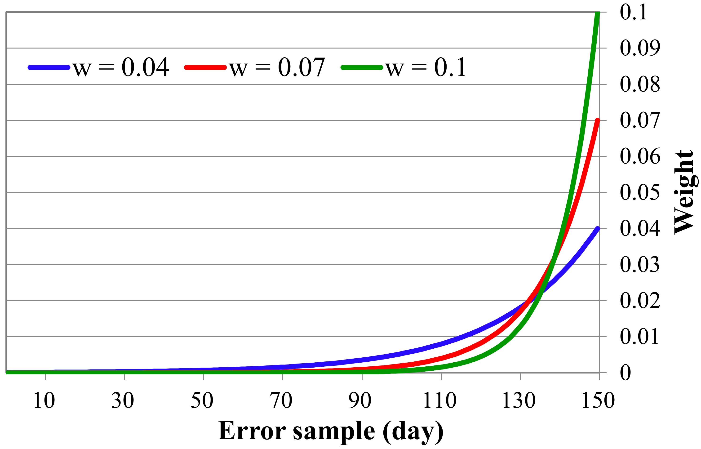
2.1. Decaying Average Algorithm

Chen and Hong [35] demonstrated the capability of a decaying average algorithm [36] to calibrate the surface temperature forecast around complex orography in Taiwan using an operational deterministic forecast in CWB. In addition, Chen and Hong [35] conducted a sensitivity test to evaluate the weighting coefficient ranging from 0.01 to 0.1 for bias correction at the model grid and indicated that the optimal weighting coefficient is 0.04. In this study, the weighting coefficient (w) of 0.07 was adapted for the instant variability of wind speed at stations around complex orography to enhance the weighting of error samples near the analysis time (Figure 1).

The bias correction procedures of the decaying average algorithm will firstly calculate model forecast error with the forecast wind speed at the station against the observed data for each forecast hour. Secondly, the system bias for each station will be statistically accumulated from the forecast error samples with a prescribed weighting coefficient [37]. Figure 1 shows the weighted function with three different weighting coefficient variates within 150 days, given by a dynamical decay weighting depending on the distance in the forecast error sample from the analysis time. Finally, the wind speed forecast can be corrected with the latest updated statistical and dynamical system bias at each forecast hour.

To demonstrate how to best represent the system bias using a decaying average algorithm, three experiments were conducted to investigate the efficiency of bias correction for an operational ensemble system. Configurations of the three experiments will be discussed in Section 3.

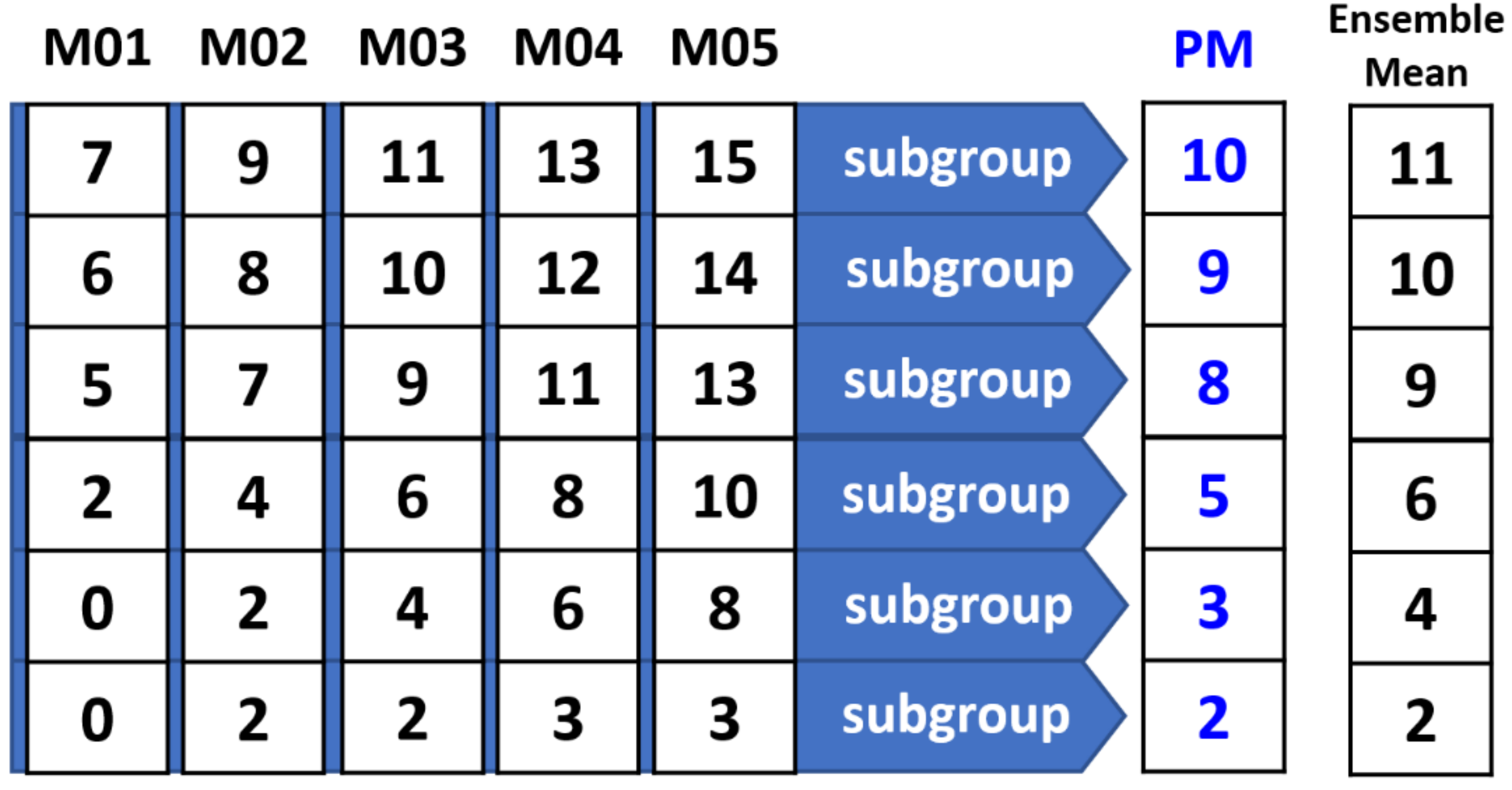
2.2. Probability Matching Mean (PMM)

The probability matched mean (PMM) method was described by Clark et al. [22] and defined to be the bias adjustment method for considering the observations [38]. This study adapted the PMM method proposed by Su et al. [26], which ranks individual ensemble members from the greatest to the smallest rainfall forecast and constitutes a subgroup with the same ranking value from each ensemble member to provide a PMM product. As mentioned, to be a bias adjustment method, the PMM product was provided based on the spatial distribution of the ensemble means and reassigned the forecast value from the subgroup referred to the observation. Figure 2 demonstrated the proposed PMM method using a 5-member ensemble with wind speed forecasts at 6 stations. In Figure 2, the value of the PM column was calculated from the average of the first quartile member (9 from M02) to the median member (11 from M03) in the same subgroup. Therefore, the maximum rank of the PM column will be 10. Finally, the station with the highest wind speed in the ensemble mean is reassigned to the highest value from the proposed PMM wind speed, and so on.

With the application of the proposed PMM method, Tsai et al. [33] improved the ensemble mean wind speed forecast from the WEPS. For the original overestimate from the WEPS, the PMM product was provided with the minimum value from the subgroup. In this study, a bias correction with the decaying average algorithm will be applied to correct the original ensemble before the application of the PMM method. Therefore, the overestimation of the original ensemble wind speed forecast could be diminished. After the bias correction, the PMM product can be provided with averaging from the first quartile to the median in a subgroup (Figure 2) for the lower bound calibrated members to cover the observational frequency. More detailed performance of the PMM products will be addressed in Section 4.

3. Materials and Experimental Design

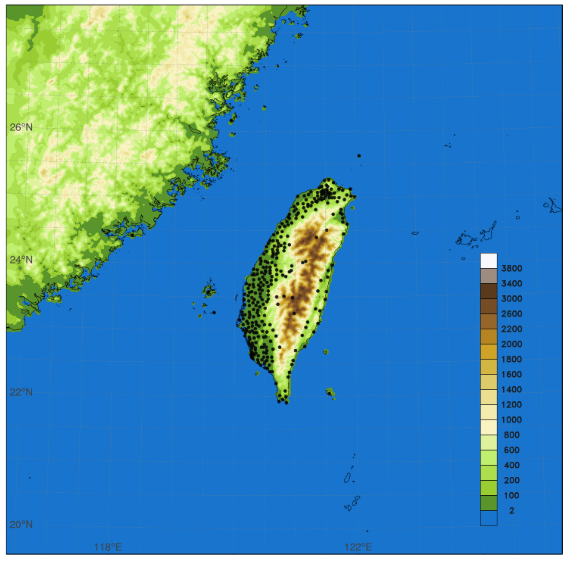
To demonstrate the efficiency of the proposed bias correction strategy for operational ensemble prediction system application, the daily ensemble forecasts from the WEPS, initiated at 0000 UTC, were collected and evaluated. In addition, how to best represent the systematic bias of the ensemble prediction system was studied via three kinds of system-bias representations. The numerical, as well as the observed data and experimental design, were described in the following subsections.

3.1. Materials

To quantitatively demonstrate the improvement to the ensemble wind speed forecast with the application of bias correction and bias adjustment, five-month (August to December in 2019) daily wind speed forecasts initialized at 0000 UTC were collected from the finest 3-km domain of Taiwan’s mesoscale ensemble prediction system [9], named WEPS. The 3-km domain of the WEPS was centered on the Taiwan cover from 19.5° N~27.9° N and 117.4° E~125.6° E as shown in Figure 3. Each member of WEPS is constructed with 52 vertical levels as well as model tops equal to 20 hPa. The model was initialized four times (0000/0600/1200/1800 UTC) a day and integrated with a time step of 60 s for a total of 72 h.

The initial and boundary condition of the 3-km domain was supplied from a coarse 15-km domain in WEPS. The initial condition of the coarse 15-km domain in WEPS combined a regional deterministic forecast, Typhoon WRF (TWRF) [39], from CWB and adding perturbations from a 32-member Ensemble Adjustment Kalman Filter (EAKF; [40]) with horizontal grid size equal to 15 km to construct the initial perturbation of the WEPS. The Typhoon WRF (TWRF) had two nested meshes with a horizontal resolution of 15/3 km and was also constructed based on the ARW WRF model [10]. TWRF was also initiated four times a day at 0000/0600/1200/1800 UTC and was run operationally at CWB since 2010. The assimilated observations of the TWRF were comprised of radiosondes, surface observations from ship and land stations, GPS radio occultation, aviation routine weather reports, and aircraft reports. More detailed configurations of the TWRF could be found in Hsiao et al. [39]. The added initial perturbations were computed as the difference between each member of the selected 20-member mean from the EAKF after a forecast time of 6 h. The lateral boundary conditions of 15 km WEPS were taken from the 10 members of the NCEP Global Ensemble Forecast System (GEFS; [41]), which means two members in the WEPS will be assigned the same boundary condition.

In this study, the ensemble 10-m wind speed forecast was collected from daily 0000 UTC and was interpolated to 316 gauges around the Taiwan area using the closest grid point, as shown in Figure 3. The model errors for each bias correction experiment were accumulated from 1 August 2019. To mimic the operational post-process procedures, the bias correction was conducted per day, and the system bias was updated daily to the end of 31 December 2019. To quantify the performance of each experiment, a month’s verification result from December 2019 will be discussed. In general, an intensive northeastern wind dominates in December in Taiwan. Observational 10-m wind speed data was hourly measured from the synoptic and automatic stations maintained by CWB in Taiwan.

3.2. Experimental Design

As mentioned, an ensemble prediction system might have systematic bias introduced from the model configurations. Therefore, a suitable bias correction strategy for an operational ensemble prediction system should be developed and evaluated. Tsai et al. [33] indicated that the bias adjustment method with PMM can reduce the wind speed forecast error, but the diurnal error characteristic remained unsolved. This study proposed three experiments corresponding to three kinds of system-bias representation with a decaying average algorithm to calibrate the original ensemble (oEPS).

One of the three experiments in

Table 1. Configuration of the experiments for bias correction using a decaying average algorithm.

Exp.	Bias Correction with Decaying Average Algorithm
oEPS	None
BC01	System bias from a single model error of the original ensemble mean.
BC03	System bias was represented by 3 model errors from each mean of PBL groups.
BC20	System bias was represented by the independent member
BC01PM	Deterministic product from BC01
BC03PM	Deterministic product from BC03
BC20PM	Deterministic product from BC20

, named BC01, corrects each ensemble forecast with system bias represented by the forecast error of the original ensemble mean. We defined the forecast error (err) as the wind speed (v) forecast against the observation at gauges (obs) in Equation (1):

err(c, m, t) = v(c, m, t) – obs(c, t)

(1)

• c = 153 cases; t = 0~72 h; m = 1,24;
• m = 1~20: for 20 members;
• m = 21: the ensemble mean;
• m = 22: the mean of members using YSU PBL;
• m = 23: the mean of members using MYNN2 PBL;
• m = 24: the mean of members using MYJ PBL.

For experiment BC01, system bias (sb) was represented by the model error accumulated from the ensemble mean as in Equation (2):

$$\mathrm{sb}(1,\mathrm{sbc},\mathrm{t})= {{\displaystyle \sum }}_{c=1}^{c=sbc}[(err\left(c,m,t\right))·cf\left(c\right)]$$

(2)

where sbc = 2~153 cases; t = 0~72 h; m = 21, the ensemble mean; and cf(c) is the weighting coefficient of model error samples in the decaying average algorithm.

Each member of the ensemble after the bias correction can be represented by Equation (3):

bc_v(sbc, m, t) = v(sbc, m, t) – sb(1, sbc, t)

(3)

where sbc = 2~153 cases; m = 1~20 for each member of the calibrated ensemble BC01.

Since the first forecast errors within 0 to 24 forecast hours were available at sbc = 2, only the 0 to 24 forecasted hourly wind speed at sbc = 2 was corrected.

The other two experiments (BC03/BC20) consider more than one model error to represent the system bias. BC03 takes three model errors independently accumulated from each mean of the PBL group and corrects the members in the same PBL group. The mathematic notation of BC03/BC20 is the same as BC01, but the system bias was represented by Equation (4)–(6) for the BC03 experiment. The calibrated ensemble in the BC03 experiment was also shown in Equations (7)–(9). Similar to BC03, the BC20 experiment will have 20 model errors for each member to represent the system bias (equations not shown).

$$\mathrm{sb}(1,\mathrm{sbc},\mathrm{t})={{\displaystyle \sum }}_{c=1}^{c=sbc}[(err\left(c,m,t\right))·cf\left(c\right)] ; \mathrm{m}=22: \mathrm{mean} \mathrm{of} \mathrm{YSU} \mathrm{PBL} \mathrm{members}$$

(4)

$$\mathrm{sb}(2,\mathrm{sbc},\mathrm{t})={{\displaystyle \sum }}_{c=1}^{c=sbc}[(err\left(c,m,t\right))·cf\left(c\right)] ; \mathrm{m}=23: \mathrm{mean} \mathrm{of} \mathrm{MYNN}2 \mathrm{PBL} \mathrm{members}$$

(5)

$$\mathrm{sb}(3,\mathrm{sbc},\mathrm{t})={{\displaystyle \sum }}_{c=1}^{c=sbc}[(err\left(c,m,t\right))·cf\left(c\right)] ; \mathrm{m}=24: \mathrm{mean} \mathrm{of} \mathrm{MYJ} \mathrm{PBL} \mathrm{members}$$

(6)

bc_v(sbc, m, t) = v(sbc, m, t) – sb(1, sbc, t); m = 1,2,11 for YSU PBL members

(7)

bc_v(sbc, m, t) = v(sbc, m, t) – sb(2, sbc, t); m = 8~10,17~20 for MYNN2 PBL members

(8)

bc_v(sbc, m, t) = v(sbc, m, t) – sb(3, sbc, t); m = 3~7,12~16 for MYJ PBL members

(9)

where sbc = 2~153 cases; t = 0~72h; and cf(c) is the weighting coefficient of model error samples in the decaying average algorithm.

After conducting bias correction, the proposed probability matched mean (PMM) method was then applied to the calibrated ensembles to provide three deterministic forecasts (BC01PM/BC03PM/BC20PM). Therefore, not only the improved probability forecast but an enhanced deterministic forecast could be provided from the Taiwan mesoscale ensemble prediction system (WEPS).

4. Results

First, the verification result for the original ensemble wind speed forecast (oEPS) as the baseline will be demonstrated. Second, the efficiency of the bias correction strategy with three kinds of system-bias representations will be shown. As the ensemble forecast was calibrated, the proposed PMM method was further applied to reconstruct the PDF of the ensemble mean from the ensemble members. Finally, a suitable bias correction strategy for operational application was proposed.

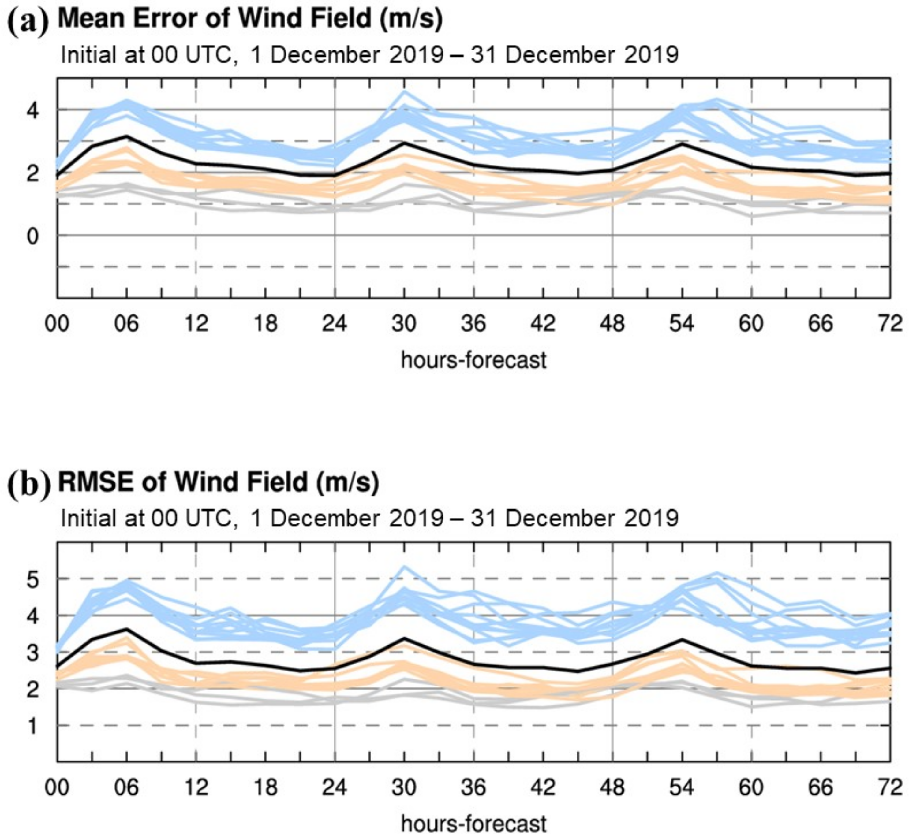
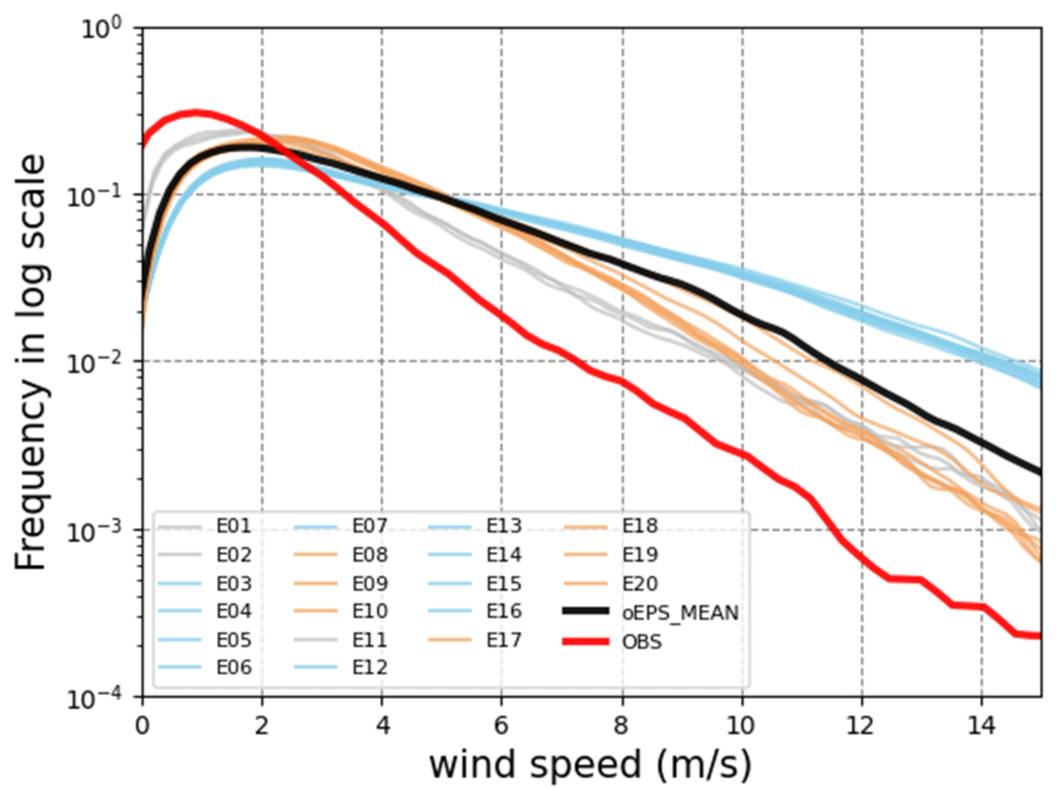
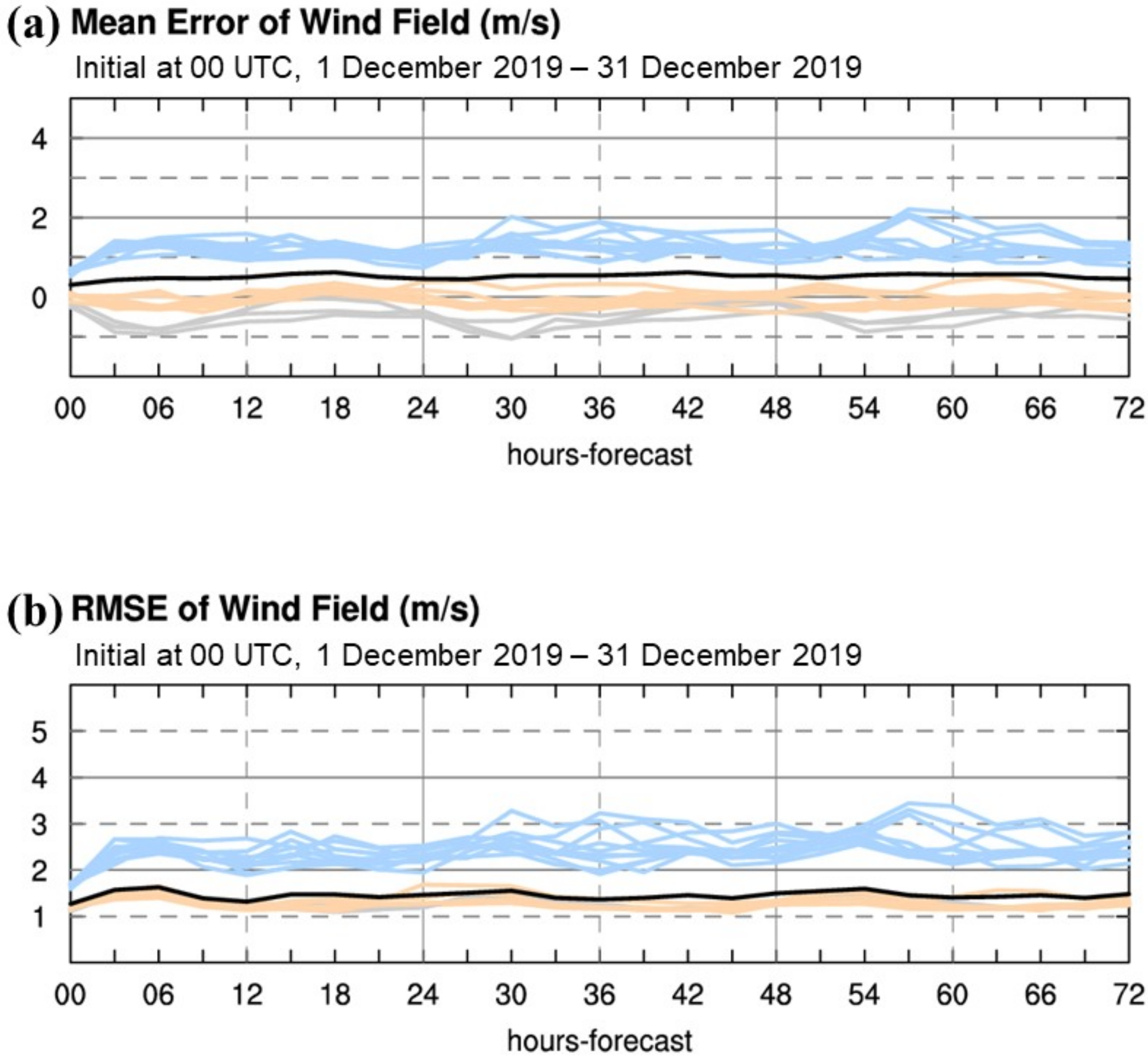
4.1. Verification of the Original Ensemble Forecast (oEPS)

The original ensemble (oEPS) wind speed forecast error was the baseline for the following calibrated ensembles. Figure 4 shows that a monthly mean error (ME) and root mean square error (RMSE) of the oEPS were clustered, resulting from the usage of the model planetary boundary layer (PBL) schemes. Members with Mellor-Yamada-Janjic (MYJ; [42,43,44]) PBL scheme had poor 10-m wind speed forecast ability and were highly overpredicted. The other two PBL schemes, Yonsei University (YSU; [45]) and Mellor-Yamada-Nakanishi and Niino Level 2.5 (MYNN2; [46,47]), performed better but slightly overpredicted. In addition, results demonstrated that model bias was diurnally variated and significantly overpredicted during the daytime. The time-averaged mean error and RMSE of the ensemble mean from oEPS with all forecast hours included were 2.29 and 2.8 (m/s).

The diagnosis of the probability density function (PDF) from the oEPS (Figure 5) also indicated that the PDF of each member was clustered concerning different PBL parameterization schemes. For wind speeds ranging from 4 to 15 m/s, the ensemble mean forecast demonstrated overprediction, resulting from the high frequency from each member. On the other hand, the wind speed forecast was slightly underpredicted within the wind speed <2 m/s. In addition, the verification results with the time average of each member and each mean of the PBL group as well as the ensemble mean are listed in

Table 2. Verification results of mean error (ME) and RMSE for the original ensemble forecast, the calibrated ensemble, and the deterministic forecast with the PM method.

	oEPS		BC01		BC03		BC20
	ME	RMSE	ME	RMSE	ME	RMSE	ME	RMSE
MEAN	2.29	2.80	0.52	1.45	0.30	1.34	0.31	1.34
E01	1.13	1.87	-0.46	1.27	0.17	1.21	0.14	1.19
E02	1.01	1.80	-0.55	1.29	0.07	1.20	0.14	1.20
E11	1.13	1.89	-0.46	1.28	0.18	1.24	0.16	1.22
YSU_MEAN	1.09	1.75	-0.49	1.18	0.14	1.08	0.14	1.08
E08	1.68	2.26	-0.05	1.27	0.17	1.25	0.18	1.25
E09	1.54	2.15	-0.16	1.25	0.06	1.22	0.18	1.24
E10	1.64	2.21	-0.10	1.21	0.13	1.20	0.17	1.21
E17	1.96	2.57	0.20	1.43	0.43	1.51	0.23	1.39
E18	1.59	2.19	-0.13	1.25	0.09	1.23	0.18	1.24
E19	1.72	2.34	-0.01	1.31	0.21	1.33	0.20	1.30
E20	1.62	2.22	-0.10	1.25	0.12	1.24	0.16	1.24
MYNN2_MEAN	1.68	2.16	-0.05	1.11	0.17	1.11	0.19	1.11
E03	3.10	3.89	1.23	2.46	0.47	2.01	0.45	1.99
E04	3.14	3.96	1.27	2.52	0.49	2.07	0.46	2.02
E05	2.93	3.72	1.08	2.33	0.33	1.92	0.43	1.95
E06	3.10	3.92	1.24	2.49	0.47	2.05	0.48	2.04
E07	3.27	4.07	1.38	2.59	0.59	2.11	0.48	2.04
E12	3.05	3.82	1.18	2.39	0.42	1.94	0.46	1.95
E13	3.15	3.92	1.28	2.47	0.50	2.00	0.46	1.96
E14	2.97	3.77	1.12	2.36	0.36	1.93	0.45	1.96
E15	3.08	3.84	1.21	2.39	0.43	1.94	0.44	1.94
E16	3.01	3.74	1.14	2.29	0.36	1.85	0.41	1.86
MYJ_MEAN	3.08	3.74	1.21	2.26	0.44	1.80	0.45	1.80
PM	–	–	0.003	1.19	0.021	1.25	0.034	1.25

, and the clusters resulting from the PBL schemes are embedded with the same background color.

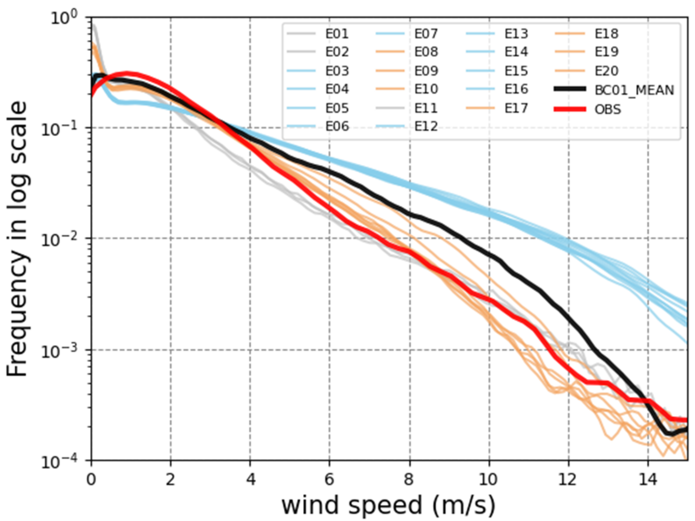
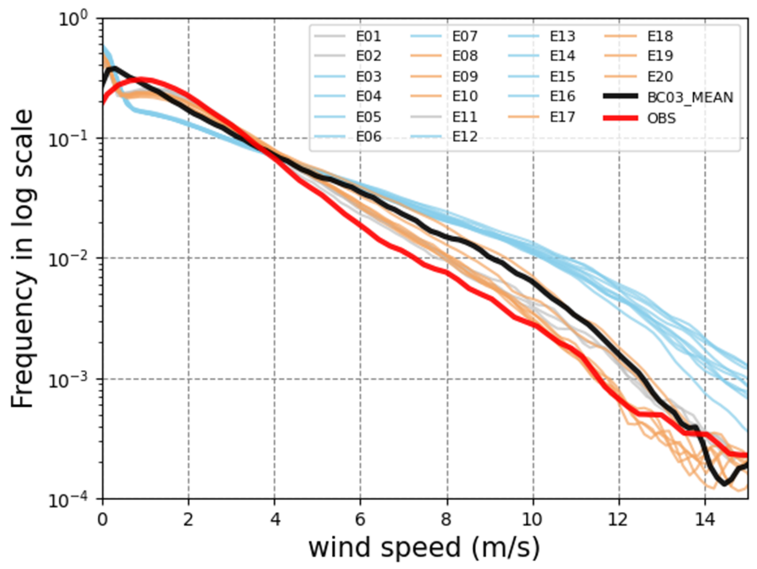
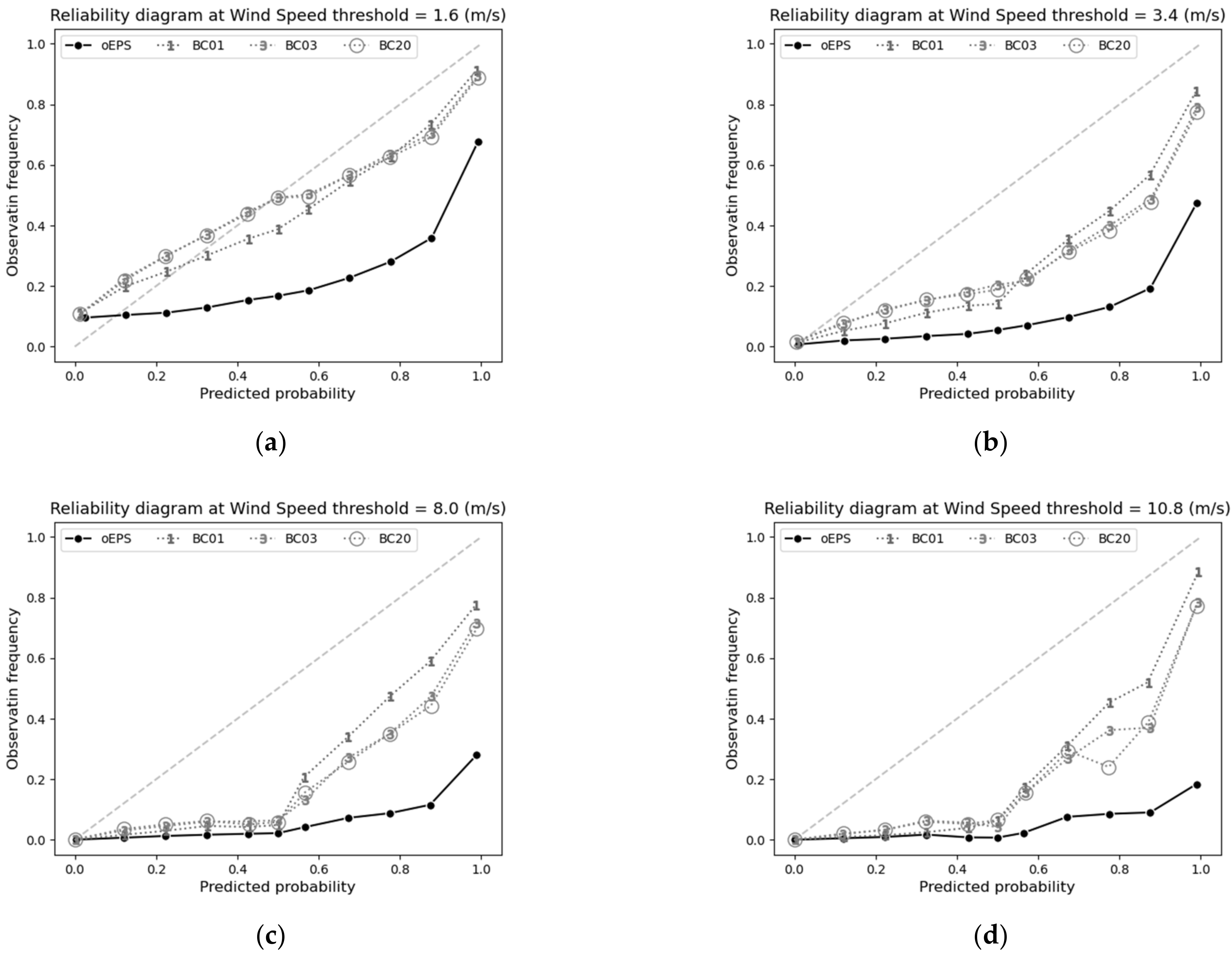
4.2. Verification of the Three Calibrated Ensemble Forecasts

To study the sensitivity of system-bias representations in an ensemble prediction system, three bias correction strategies (BC01/BC03/BC20) with decaying average algorithms corresponded with 3-type system biases were configured. Verification results showed that the forecast bias of the ensemble mean of BC01 was significantly reduced when the system bias was represented by the single model error from the original ensemble mean. In Figure 6, to emphasize the effect of the decaying average algorithm bias correction with time-dependent model bias characteristic, the monthly averaged wind speed forecast ME and RMSE for each forecast hour with 31 cases were demonstrated. Furthermore, the time-averaged ME and RMSE of the means of BC01 were 0.52 and 1.45 m/s, which were significantly reduced from 2.29 and 2.8 m/s of the oEPS. In addition to the improvement of accuracy, the diurnal variability of error characteristic was successfully eliminated. In

Table 3. The mean error, RMSE, and the ensemble spread of the original as well as the calibrated ensembles.

Experiments	ME	RMSE	SPREAD
oEPS	2.29	2.80	1.32
BC01	0.52	1.45	1.15
BC03	0.30	1.34	0.89
BC20	0.31	1.34	0.86

, the ensemble spread of BC01 was slightly reduced to 1.15 m/s from 1.32, but BC01 remained capable of being applied to the probability forecast in comparison with BC03 and BC20. Moreover, the probability density function (PDF) also showed improvements in the calibrated ensemble. In Figure 7, the high-frequency wind speed within 4 to 15 m/s was reduced in each member. Although members of the MYJ PBL scheme remained overpredicted, the other two PBL schemes can be calibrated to cover the frequency of the observed wind speed, especially in ranges from 4 to 15 m/s. In addition, the wind speed weaker than 2 m/s can also benefit from the bias correction in BC01.

Members of the experiment, BC03, were calibrated with system bias collected from three model errors. Three model errors (Equations (4)–(6)) were calculated from the mean of each PBL group, and then each member in the same PBL group was corrected respectively (Equations (7)–(9)). As the original ensemble demonstrated, three clusters in the verification, BC03 with three-kind model errors to represent the system bias was expected to better represent the error characteristics of the oEPS. In Figure 8, the time-averaged ME and RMSE of the ensemble mean in BC03 can be further reduced to 0.3 and 1.34 m/s, and the clustering error characteristic could be diminished compared to BC01. However, the ensemble spread in BC03 was shrunk from 1.32 to 0.89 m/s resulted in an insufficient ensemble spread. On the other hand, the PDF of BC03 indicated that the high wind speed frequency between 4 to 15 m/s can be reduced, but members with the MYJ PBL scheme are still overpredicted. For wind speeds within 4 to 15 m/s, the calibrated members seldom mimic the observed frequency but only the extreme wind speed situation within 10 to 15 m/s (Figure 9).

The experiment, BC20, with the system bias calculated for each independent member, was expected to be the best forecast experiment. Results, as expected, indicated that the ensemble mean of BC20 was similar to that of BC03 and the time average ME and RMSE were 0.3 and 1.34 m/s. However, the ensemble spread of BC20 was the smallest and equaled 0.86 (m/s) in Table 3, and the verification of PDF also demonstrated an insufficient ensemble spread (figures not shown).

To further diagnose the performance of calibrated ensembles (BC01/BC03/BC20), the probability forecasts of all the ensembles were evaluated over several wind speed thresholds. In Figure 10, the probability forecast in different wind speed thresholds was shown from the Beaufort (BF) scales 2 to 6. For the BF scales equal to 2 (Figure 10a), all the calibrated ensembles improve the reliability for each predicted probability, although the BC01 slightly degraded at around 0.5 thresholds. As the wind speed threshold increased (Figure 10b–d), the higher predicted probability also benefited from the bias correction, especially in the BC01, which remained the greatest ensemble spread with a suitable spread-error ratio. Therefore, a more reliable risk assessment, as well as earned value analysis, can be achieved resulting from the calibrated ensemble (BC01). Furthermore, all the calibrated ensemble products at the predicted probability threshold greater than 0.5 were significantly improved, which might result from the correction of the 10 members with the MYJ PBL scheme.

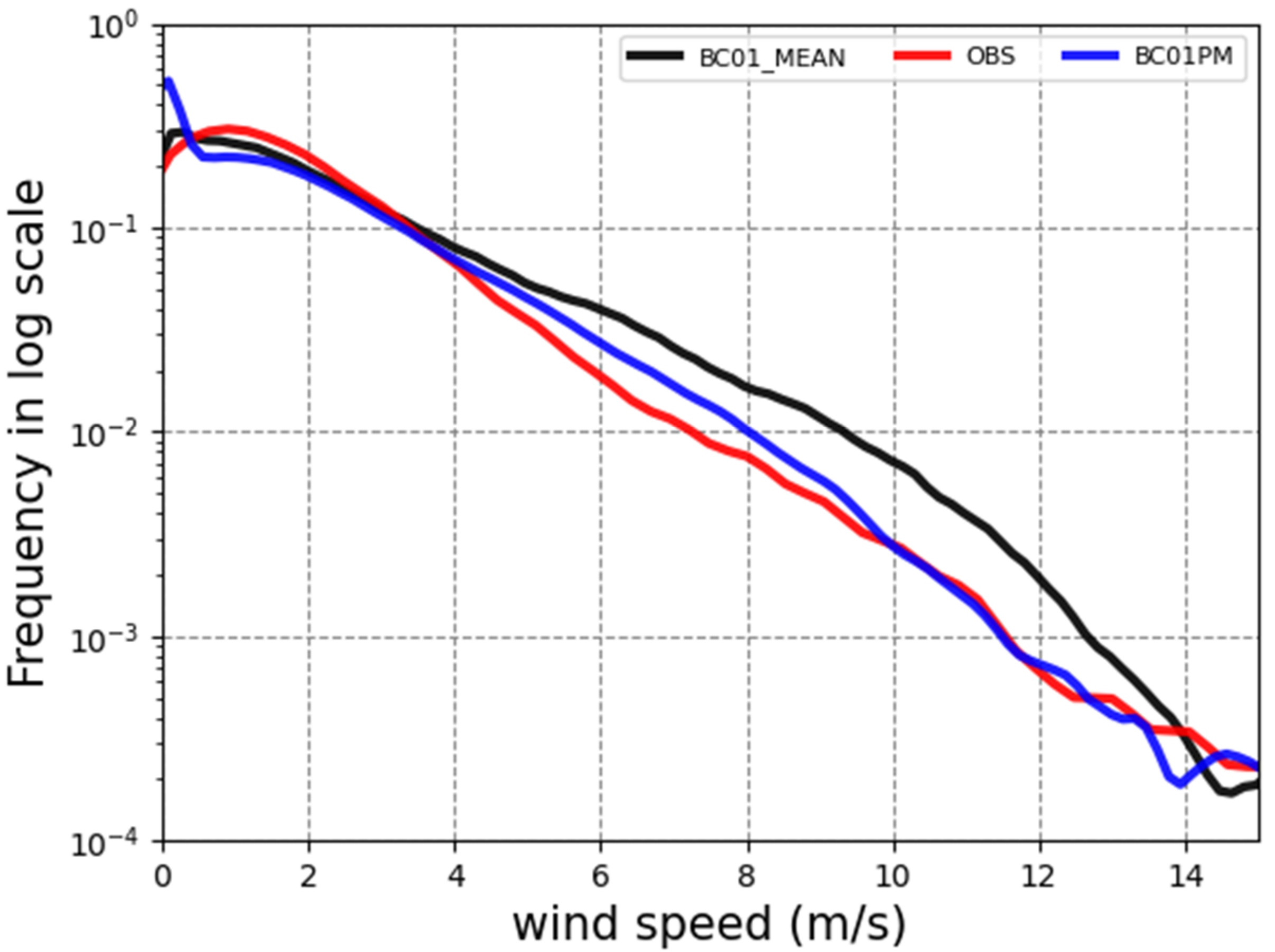
4.3. Verification of Probability Matched Mean (PMM) Products

After conducting the bias correction, the probability matched mean (PMM) method was applied to the three calibrated ensembles to provide deterministic forecast products (BC01PM/BC03PM/BC20PM). In Figure 7, although the PDF of the calibrated ensemble (BC01) was improved, the mean of the calibrated ensemble still shows high frequency within the range from 4 to 14 m/s. Moreover, the mean of the calibrated ensemble is generally located in the median, and the lower 10 calibrated members can approximately cover the observation frequency. Therefore, the proposed probability matched mean (PMM) product will be based on the spatial distribution of the mean of the calibrated ensemble and reconstruct the PDF from the calibrated members using the average from the first quartile to the median.

Figure 11 shows that the proposed PMM method can further improve the PDF, especially within the wind speed range from 4 to 14 m/s based on the mean of the calibrated ensemble (BC01). Among the three deterministic forecast products (Figure 12), the BC01PM, resulting from a calibrated ensemble with a suitable spread-error ratio, can significantly reduce the RMSE by about 18% from 1.45 to 1.19 m/s and unbias the forecast error (mean error equals 0.003 m/s). The other two deterministic forecasts (BC03PM and BC20PM) can also unbiased the wind speed forecast, but the accuracy improvement of 7% resulted from the insufficient ensemble spread. Moreover, the other PMM strategy with the value exactly equal to the first quartile in a subgroup was also evaluated but will introduce negative bias (figure not shown).

5. Discussion and Conclusion

In this study, 10-m wind speed forecasts from the Taiwan mesoscale ensemble prediction system, also named WEPS, were investigated. The 3-km 20-member WEPS system consists of initial, lateral boundary, and model perturbations, including multi-physics and two stochastic perturbation schemes (SKEB and SPPT). First of all, the 10-m wind speed forecast was verified against surface observations. The error exhibited diurnal variation and clustered concerning the selected PBL scheme in different ensemble members. To correct this systematic bias to improve the wind speed forecast, three experiments that utilized decaying average algorithm were configured:

(a)

BC01: System bias from a single model error of the original ensemble mean.

(b)

BC03: System bias was represented by three model errors from each mean of PBL groups.

(c)

BC20: System bias was represented by the independent member.

Since model forecasts with higher accuracy are always desirable for operational application, the calibrated wind speed from the three experiments that address different kinds of systematic bias are compared. In general, the decaying average algorithm eliminated the diurnal error characteristic of the ensemble wind speed forecast. Moreover, the RMSE of the mean from the calibrated ensemble means (BC01/BC03/BC20) were significantly reduced to 1.45, 1.34, and 1.34 m/s, respectively. Although the RMSE of the calibrated ensemble mean (BC01) was slightly degraded, it remains the largest ensemble spread (1.15) among the three experiments (BC03 equals 0.89 and BC20 equals 0.86). The spread-error ratio of each corrected ensemble indicated that the calibrated ensemble (BC01) with model bias calculated from the ensemble mean of oEPS is the most reliable. Furthermore, a similar conclusion was obtained from the reliability diagram of each calibrated ensemble in different Beaufort Scale thresholds. As the reliability of the probability forecast was enhanced, it could precisely identify the specific wind event and save a much more economic value from a corresponding suitable action. In addition, the probability matched mean (PMM) method was applied to reconstruct the PDF of the calibrated ensemble mean from the corrected members. At the same time, the combination of bias correction and bias adjustment techniques is expected to advance the calibrated accuracy. Verification results show that the error and bias of the ensemble mean were greatly corrected by applying the decaying average algorithm. Furthermore, the mean of the three calibrated ensembles with bias adjustment (PMM) applied (BC01PM/BC03PM/BC20PM) were almost unbiased and their accuracy was even further improved. Among the three PMM products, BC01PM was the best result from the suitable spread-error relation of the calibrated ensemble (BC01).

To sum up, the application of the bias correction (decaying average algorithm) as well as bias adjustment (PMM) to a WRF ensemble prediction system was investigated, and a suitable bias correction strategy was proposed for operational usage. Results indicated that applying the proposed bias correction first is essential to retain the ensemble spread. Afterward, applying a bias adjustment (PMM) method can produce an unbiased deterministic forecast. Currently, the bias correction strategy proposed in this study is semi-operated for WEPS in Taiwan. A strong wind event with a duration of almost a month in Jun. 2021 was evaluated. Against the same 316 stations, the original ensemble mean wind speed forecast had a mean error (ME), and root mean square error (RMSE) of 1.33 and 2.1 m/s. After bias correction with the system bias represented by the original ensemble mean, the ME and RMSE were reduced to 0.24 and 1.41 m/s, respectively. Finally, combined with the bias adjustment (PMM) method, the ME and RMSE of the calibrated ensemble could be further reduced (0.08 and 1.16 m/s).

In this study, the combination of bias correction and bias adjustment techniques was proved robust to improve ensemble wind speed forecast. In the future, we plan to further explore the sensitivity of the prescribed weighting coefficient in the decaying average algorithm. Furthermore, since the artificial intelligence (AI) methods have been widely used in the science community [34,48], their application in ensemble post-process should be further explored. For example, several deep learning methods, such as micro-genetic algorithms or random forests, can also be applied to correct systematic bias in ensemble forecasts. Since the proposed renewable energy policy in Taiwan tends to phase out nuclear power gradually, a more accurate wind prediction provided by the proposed bias correction and bias adjustment strategy in this study can be applied to the wind forecast at altitudes of wind turbines. This could contribute to decision making for wind farm operators, reduce the imbalance to the power grids, and improve the efficiency of wind power forecasts.

References

1. Wyszogrodzki, A.A.; Liu, Y.; Jacobs, N.; Childs, P.; Zhang, Y.; Roux, G.; Warner, T.T. Analysis of the surface temperature and wind forecast errors of the NCAR-AirDat operational CONUS 4-km WRF forecasting system. Theor. Appl. Clim. 2013, 122, 125–143. [Google Scholar] [CrossRef] [Green Version]
2. Olson, J.B.; Kenyon, J.S.; Djalalova, I.; Bianco, L.; Turner, D.; Pichugina, Y.; Choukulkar, A.; Toy, M.D.; Brown, J.M.; Angevine, W.M.; et al. Improving Wind Energy Forecasting through Numerical Weather Prediction Model Development. Bull. Am. Meteorol. Soc. 2019, 100, 2201–2220. [Google Scholar] [CrossRef]
3. Fovell, R.G.; Gallagher, A. Boundary Layer and Surface Verification of the High-Resolution Rapid Refresh, Version 3. Weather Forecast. 2020, 35, 2255–2278. [Google Scholar] [CrossRef]
4. Zhang, D.L.; Zheng, W.Z. Diurnal cycles of surface winds and temperatures as simulated by five boundary layer parameterizations. J. Appl. Meteorol. 2004, 43(1), 157–169. [Google Scholar] [CrossRef] [Green Version]
5. Deppe, A.J.; Gallus, W.A.; Takle, E.S. A WRF Ensemble for Improved Wind Speed Forecasts at Turbine Height. Weather Forecast. 2013, 28, 212–228. [Google Scholar] [CrossRef]
6. Heppelmann, T.; Steiner, A.; Vogt, S. Application of numerical weather prediction in wind power forecasting: Assessment of the diurnal cycle. Meteorol. Z. 2017, 26, 319–331. [Google Scholar] [CrossRef]
7. Schwartz, C.S.; Romine, G.S.; Sobash, R.A.; Fossell, K.R.; Weisman, M.L. NCAR’s Experimental Real-Time Convection-Allowing Ensemble Prediction System. Weather Forecast. 2015, 30, 1645–1654. [Google Scholar] [CrossRef]
8. Schwartz, C.S.; Wong, M.; Romine, G.S.; Sobash, R.A.; Fossell, K.R. Initial Conditions for Convection-Allowing Ensembles over the Conterminous United States. Mon. Weather Rev. 2020, 148, 2645–2669. [Google Scholar] [CrossRef] [Green Version]
9. Li, C.-H.; Berner, J.; Hong, J.-S.; Fong, C.-T.; Kuo, Y.-H. The Taiwan WRF Ensemble Prediction System: Scientific Description, Model-Error Representation and Performance Results. Asia-Pac. J. Atmos. Sci. 2019, 56, 1–15. [Google Scholar] [CrossRef] [Green Version]
10. Skamarock, W.C.; Klemp, J.B.; Dudhia, J.; Gil, D.A.; Barker, D.M.; Duda, M.G.; Huang, X.Y.; Wang, W.; Powers, J.G. Description of the Advanced Research WRF Version 3 (No. NCAR/TN-475+STR); National Center for Atmospheric Research: Boulder, CO, USA, 2008. [Google Scholar] [CrossRef]
11. Li, C.-H.; Hong, J.-S. The study of regional ensemble forecast: Evaluation for the performance of perturbed methods. Atmos. Sci. 2014, 42, 153–179, (In Chinese with English abstract). [Google Scholar]
12. Berner, J.; Ha, S.-Y.; Hacker, J.P.; Fournier, A.; Snyder, C.S. Model Uncertainty in a Mesoscale Ensemble Prediction System: Stochastic versus Multiphysics Representations. Mon. Weather Rev. 2011, 139, 1972–1995. [Google Scholar] [CrossRef] [Green Version]
13. Berner, J.; Fossell, K.R.; Ha, S.-Y.; Hacker, J.P.; Snyder, C. Increasing the Skill of Probabilistic Forecasts: Understanding Performance Improvements from Model-Error Representations. Mon. Weather Rev. 2015, 143, 1295–1320. [Google Scholar] [CrossRef]
14. Shutts, G. A kinetic energy backscatter algorithm for use in ensemble prediction systems. Q. J. R. Meteorol. Soc. 2005, 131, 3079–3102. [Google Scholar] [CrossRef] [Green Version]
15. Buizza, R.; Milleer, M.; Palmer, T.N. Stochastic representation of model uncertainties in the ECMWF ensemble prediction system. Q. J. R. Meteorol. Soc. 1999, 125, 2887–2908. [Google Scholar] [CrossRef]
16. Palmer, T.N.; Buizza, R.; Doblas-Reyes, F.; Jung, T.; Leutbecher, M.; Shutts, G.; Steinheimer, M.; Weisheimer, A. Stochastic parametrization and model uncertainty. ECMWF Tech. Memo. 2009, 598, 2–17. Available online: https://www2.physics.ox.ac.uk/sites/default/files/2011-08-15/techmemo598_stochphys_2009_pdf_50419.pdf (accessed on 25 October 2021).
17. Murphy, A.H. Skill scores based on the mean square error and their relationships to the correlation coefficient. Mon. Weather Rev. 1988, 116, 2417–2424. [Google Scholar] [CrossRef]
18. Snyder, C.; Zhang, F. Assimilation of Simulated Doppler Radar Observations with an Ensemble Kalman Filter. Mon. Weather Rev. 2003, 131, 1663–1677. [Google Scholar] [CrossRef] [Green Version]
19. Ruiz, J.; Saulo, C.; Nogués-Paegle, J. WRF Model Sensitivity to Choice of Parameterization over South America: Validation against Surface Variables. Mon. Weather Rev. 2010, 138, 3342–3355. [Google Scholar] [CrossRef]
20. Snook, N.; Kong, F.; Brewster, K.A.; Xue, M.; Thomas, K.W.; Supinie, T.A.; Perfater, S.; Albright, B. Evaluation of Convection-Permitting Precipitation Forecast Products Using WRF, NMMB, and FV3 for the 2016–17 NOAA Hydrometeorology Testbed Flash Flood and Intense Rainfall Experiments. Weather Forecast. 2019, 34, 781–804. [Google Scholar] [CrossRef] [Green Version]
21. Ebert, E.E. Ability of a Poor Man’s Ensemble to Predict the Probability and Distribution of Precipitation. Mon. Weather Rev. 2001, 129, 2461–2480. [Google Scholar] [CrossRef]
22. Clark, A.J.; Gallus, W.A.; Xue, M.; Kong, F. A Comparison of Precipitation Forecast Skill between Small Convection-Allowing and Large Convection-Parameterizing Ensembles. Weather Forecast. 2009, 24, 1121–1140. [Google Scholar] [CrossRef] [Green Version]
23. Xue, M.; Kong, F.; Tomas, K.W.; Wang, Y.; Brewster, K.; Gao, J.; Wang, X.; Weiss, S.J.; Clark, A.; Kain, J.S.; et al. Realtime convection-permitting ensemble and convection-resolving deterministic forecasts of CAPS for the Hazardous Weather Testbed 2010 Spring Experiment. In 24th Conference on Weather and Forecasting/20th Conference on Numerical Weather Prediction, Seattle, WA, USA, 22–27 January 2011; American Meteorology Society: Seattle, WA, USA, 2011. [Google Scholar]
24. Fang, X.; Kuo, Y.-H. Improving Ensemble-Based Quantitative Precipitation Forecasts for Topography-Enhanced Typhoon Heavy Rainfall over Taiwan with a Modified Probability-Matching Technique. Mon. Weather Rev. 2013, 141, 3908–3932. [Google Scholar] [CrossRef] [Green Version]
25. Schwartz, C.S.; Romine, G.S.; Smith, K.R.; Weisman, M.L. Characterizing and Optimizing Precipitation Forecasts from a Convection-Permitting Ensemble Initialized by a Mesoscale Ensemble Kalman Filter. Weather Forecast. 2014, 29, 1295–1318. [Google Scholar] [CrossRef] [Green Version]
26. Su, Y.J.; Hong, J.S.; Li, C.H. The Characteristics of the Probability Matched Mean QPF for 2014 Meiyu Season. Atmos. Sci. 2016, 44, 113–134, (In Chinese with English abstract). [Google Scholar]
27. Qiao, X.; Wang, S.; Schwartz, C.S.; Liu, Z.; Min, J. A Method for Probability Matching Based on the Ensemble Maximum for Quantitative Precipitation Forecasts. Mon. Weather Rev. 2020, 148, 3379–3396. [Google Scholar] [CrossRef]
28. Snook, N.; Kong, F.; Clark, A.; Roberts, B.; Brewster, K.A.; Xue, M. Comparison and Verification of Point-Wise and Patch-Wise Localized Probability-Matched Mean Algorithms for Ensemble Consensus Precipitation Forecasts. Geophys. Res. Lett. 2020, 47, e2020GL087839. [Google Scholar] [CrossRef]
29. Junk, C.; Von Bremen, L.; Kühn, M.; Späth, S.; Heinemann, D. Comparison of Postprocessing Methods for the Calibration of 100-m Wind Ensemble Forecasts at Off- and Onshore Sites. J. Appl. Meteorol. Clim. 2014, 53, 950–969. [Google Scholar] [CrossRef]
30. Junk, C.; Späth, S.; von Bremen, L.; Monache, L.D. Comparison and Combination of Regional and Global Ensemble Prediction Systems for Probabilistic Predictions of Hub-Height Wind Speed. Weather Forecast. 2015, 30, 1234–1253. [Google Scholar] [CrossRef] [Green Version]
31. Mittermaier, M.P.; Csima, G. Ensemble versus Deterministic Performance at the Kilometer Scale. Weather Forecast. 2017, 32, 1697–1709. [Google Scholar] [CrossRef]
32. Chen, S.-H.; Yang, S.-C.; Chen, C.-Y.; van Dam, C.; Cooperman, A.; Shiu, H.; MacDonald, C.; Zack, J. Application of bias corrections to improve hub-height ensemble wind forecasts over the Tehachapi Wind Resource Area. Renew. Energy 2019, 140, 281–291. [Google Scholar] [CrossRef]
33. Tsai, C.C.; Su, Y.J.; Li, C.H.; Chang, B.L.; Hong, J.S. Optimizing the Ensemble Wind Speed Forecast with Probability Matched Mean Method. In Proceedings of the 2020 Conference on Weather Analysis and Forecasting, Taipei, Taiwan, 13–15 October 2020. (In Chinese with English abstract). [Google Scholar]
34. Goutham, N.; Alonzo, B.; Dupré, A.; Plougonven, R.; Doctors, R.; Liao, L.; Mougeot, M.; Fischer, A.; Drobinski, P. Using Machine-Learning Methods to Improve Surface Wind Speed from the Outputs of a Numerical Weather Prediction Model. Boundary-Layer Meteorol. 2021, 179, 133–161. [Google Scholar] [CrossRef]
35. Chen, Y.R.; Hong, J.S. Bias Correction of Surface Temperature Prediction by Using the Decaying Average Algorithm. Atmos. Sci. 2017, 45, 25–42, (In Chinese with English abstract). [Google Scholar]
36. Cui, B.; Tóth, Z.; Zhu, Y.; Hou, D. Bias Correction for Global Ensemble Forecast. Weather Forecast. 2012, 27, 396–410. [Google Scholar] [CrossRef]
37. Glahn, B. Determining an Optimal Decay Factor for Bias-Correcting MOS Temperature and Dewpoint Forecasts. Weather Forecast. 2014, 29, 1076–1090. [Google Scholar] [CrossRef]
38. Clark, A.J.; Gallus, W.A.; Weisman, M.L. Neighborhood-Based Verification of Precipitation Forecasts from Convection-Allowing NCAR WRF Model Simulations and the Operational NAM. Weather Forecast. 2010, 25, 1495–1509. [Google Scholar] [CrossRef]
39. Hsiao, L.-F.; Chen, D.-S.; Hong, J.-S.; Yeh, T.-C.; Fong, C.-T. Improvement of the Numerical Tropical Cyclone Prediction System at the Central Weather Bureau of Taiwan: TWRF (Typhoon WRF). Atmosphere 2020, 11, 657. [Google Scholar] [CrossRef]
40. Anderson, J.L. An ensemble adjustment Kalman filter for data assimilation. Mon. Weather Rev. 2001, 129, 2884–2903. [Google Scholar] [CrossRef] [Green Version]
41. Ei, M.W.; Oth, Z.O.T.; Obus, R.I.W.; Zhu, Y. Initial perturbations based on the ensemble transform (ET) technique in the NCEP global operational forecast system. Tellus A: Dyn. Meteorol. Oceanogr. 2008, 60, 62–79. [Google Scholar] [CrossRef] [Green Version]
42. Janjić, Z.I. The Step-Mountain Coordinate: Physical Package. Mon. Weather Rev. 1990, 118, 1429–1443. [Google Scholar] [CrossRef]
43. Janjic, Z.I. The step-mountain eta coordinate model: Further developments of the convection, viscous sublayer, and turbulence closure schemes. Mon. Weather Rev. 1994, 122, 927–945. [Google Scholar] [CrossRef] [Green Version]
44. Janjic, Z. Nonsingular Implementation of the Mellor-Yamada Level 2.5 Scheme in the NCEP Meso Model; Office Note #436; National Centers for Environmental Prediction: College Park, MD, USA, 2002; p. 436. [Google Scholar]
45. Hong, S.-Y.; Noh, Y.; Dudhia, J. A New Vertical Diffusion Package with an Explicit Treatment of Entrainment Processes. Mon. Weather Rev. 2006, 134, 2318–2341. [Google Scholar] [CrossRef] [Green Version]
46. Nakanishi, M.; Niino, H. An Improved Mellor–Yamada Level-3 Model with Condensation Physics: Its Design and Verification. Boundary-Layer Meteorol. 2004, 112, 1–31. [Google Scholar] [CrossRef]
47. Nakanishi, M.; Niino, H. An Improved Mellor–Yamada Level-3 Model: Its Numerical Stability and Application to a Regional Prediction of Advection Fog. Boundary-Layer Meteorol. 2006, 119, 397–407. [Google Scholar] [CrossRef]
48. Yang, T.-H.; Tsai, C.-C. Using numerical weather model outputs to forecast wind gusts during typhoons. J. Wind. Eng. Ind. Aerodyn. 2019, 188, 247–259. [Google Scholar] [CrossRef]
Figure 1. The weighting of 150-day model error samples in different weighting coefficients (0.04, 0.07, and 0.1) with the usage.
Atmosphere 12 01688 g001
Figure 2. A 5-member ensemble system with wind speed forecast at 6 gauges to demonstrate the proposed PMM method.
Atmosphere 12 01688 g002
Figure 3. The 3-km domain of the WEPS and the 316 stations with black dots around Taiwan were used for verification; the terrain height is shaded.
Atmosphere 12 01688 g003
Figure 4. Monthly verification of the original ensemble forecast (oEPS) in forecast hour. Lines in different colors indicated the ensemble members with different PBL schemes: gray for YSU, orange for MYNN2, blue for MYJ, and black for the ensemble mean. (a) The mean error of each ensemble and (b) the RMSE.
Atmosphere 12 01688 g004
Figure 5. The probability density function of the original ensemble forecast (oEPS). Gray for YSU, orange for MYNN2, blue for MYJ, and black for the ensemble mean; the red line is the frequency of the observed wind speed.
Atmosphere 12 01688 g005
Figure 6. Monthly verification of the original ensemble forecast (BC01) in the forecast hour. Lines in different colors indicated the ensemble members with different PBL schemes: gray for YSU, orange for MYNN2, blue for MYJ, and black for the ensemble mean. (a) Mean error of each ensemble and (b) RMSE.
Atmosphere 12 01688 g006
Figure 7. The probability density function of the original ensemble forecast (BC01). Gray for YSU, orange for MYNN2, blue for MYJ, and black for the ensemble mean; the red line is the frequency of the observed wind speed.
Atmosphere 12 01688 g007
Figure 8. Monthly verification of the original ensemble forecast (BC03) in the forecast hour. Lines in different colors indicated the ensemble members with different PBL schemes: gray for YSU, orange for MYNN2, blue for MYJ, and black for the ensemble mean. (a) Mean error of each ensemble and (b) RMSE.
Atmosphere 12 01688 g008
Figure 9. The probability density function of the original ensemble forecast (BC03). Gray for YSU, orange for MYNN2, blue for MYJ, and black for the ensemble mean; the red line is the frequency of the observed wind speed.
Atmosphere 12 01688 g009
Figure 10. Reliability diagram of the original ensemble prediction (oEPS) and the 3 calibrated ensembles (BC01/BC03/BC20) in different Beaufort (BF) Scale thresholds: (a) BF equals 2, (b) equals 3, (c) equals 5, and (d) equals 6.
Atmosphere 12 01688 g010
Figure 11. Same as in Figure 4 but for the calibrated ensemble forecast, BC01, with the application of probability matched mean (PMM) method (blue). The ensemble mean of BC01 is in black, and the observed is in red.
Atmosphere 12 01688 g011
Figure 12. Monthly averaged (a) mean error and (b) RMSE of each mean from the three calibrated ensembles (BC01/BC03/BC20) in black, and the corresponding deterministic forecast (BC01PM/BC03PM/BC20PM) with PMM method applied is in blue. (BC01 with a solid line; BC03 with dash line; BC20 with dot line).
Atmosphere 12 01688 g012