A Re-Evaluation of the Swiss Hail Suppression Experiment Using Permutation Techniques Shows Enhancement of Hail Energies When Seeding

Abstract

Grossversuch IV is a large and well documented experiment on hail suppression by silver iodide seeding. The original 1986 evaluation remained vague, although indicating a tendency to increase hail when seeding. The strategy to deal with distributions of hail energy far from normal was not optimal. The present re-evaluation sticks to the question asked and avoids both misleading transformations and unsatisfactory meteorological predictors. The raw data show an increase by about a factor of 3 for the hail energy when seeding. This is the opposite of what seeding is supposed to do. The probability to obtain such a result by chance is below 1%, calculated by permutation and bootstrap techniques applied on the raw data. Confidence intervals were approximated by bootstrapping as well as by a new method called “correlation imposed permutation” (CIP).

1. Introduction

Hail damage to crops, fruits, cars, buildings and even people is a disaster which leads especially farmers to seek for protection. Silver iodide seeding from airplanes is a commercially available practice. The glaciating power of silver iodide in cold clouds is beyond doubt. It is therefore logical to try promoting snow and rainfall from cold cloud systems by introducing silver iodide that produces ice crystals growing faster than water droplets (see, for instance, the review of wintertime orographic cloud seeding in [1] and the literature cited there).

Hail suppression by silver iodide is a different issue. At first glance, it seems that introducing ice forming nuclei into thunderstorms would enhance the formation of hail. On the other hand an artificial increase of the number of hail embryos could reduce the size of hailstones and thus also the kinetic energy of hail by the competition for the available supercooled water. This idea, promoted mainly by Sulakvelidze [2], was the basis for many operational programs of hail suppression in the former USSR, in Eastern Europe and more than 20 other countries worldwide, see Figure 1 in [3]. Later, other theories for hail suppression and accordingly different seeding procedures have been put forward by Abshaev, Sulakvelidze and other protagonists of hail suppression [4]. For large supercell storms, ideas were presented by Browning and Foote [5]. They state in their conclusions “A supercell storm exhibits a kind of natural selection mechanism which tends to restrict the number of embryos, natural or artificial, entering the hail growth region. As a result the ‘hail factory’ does not work at anywhere near its full capacity and the production of additional embryos by seeding in the main updraft may increase the amount of hail rather than promote effective competition”. A comprehensive review on hail suppression by different methods was done by Wieringa and Hollemann [6], and, more recently, by Rivera et al. [3], who confirms the uncertainty about a possible benefit of 60 years of hail suppression in Mendoza (Argentina).

Adequate statistical methods should be able to prove the success or failure of hail suppression in less time. The need for such methods seems clear. The focus of the present study is on the statistical treatment of data which are most representative for hail damage. The total kinetic energy of the hail falling to the ground is a suitable choice. Unfortunately, the distribution of this variable when measured for different thunderstorm cells is far from normal. This is a real problem in different ways, for testing as well as for the size of the sample necessary to reject the null hypothesis ($H_0$), which claims that an observed effect could be accidental. The present authors are not aware of a hail suppression experiment surmounting both statistical obstacles. They were curious to apply adequate statistical methods nowadays available on modern computers to one of the larger and well documented scientific experiments on hail suppression, “Grossversuch IV” [7].

Grossversuch IV was launched by the department of agriculture of Switzerland, France and Italy, the Swiss and French hail insurance companies and it was directed by the Swiss Federal Institute of Technology (ETH). The scope was to find out by a randomized experiment whether silver iodide seeding according to the procedure used in the former USSR had a statistically significant effect on the hail energy. The experiment was carried out in the years 1977–1982 in a hilly region of about 1300 km² in the centre of Switzerland, ${47}^{\circ }$ North, $8^{\circ }$ East. The region was surveyed by two radars and a network of hailpads, the seeding performed by Soviet rockets and launchers. A total of 37 experimental days were drawn for seeding, 46 for non-seeded controls, containing 113 and 140 cells, respectively. The total hail energy on ground ($E_{GR}$) was determined for each cell by radar. Everything was done to reproduce exactly the procedure used at that time in the USSR. However, the performance of the seeding was unsatisfactory as only one half of the prescribed number of rockets were launched successfully. From the logbooks for each cell the “seeding coverage” ($sc$), the ratio of successful launches to the prescribed number of rockets or, in other terms, the fraction of the duration of correct seeding was determined. One rocket had to be fired every 5 min as long as the seeding criterion was fulfilled. The shortcoming of the seeding makes it questionable whether Grossversuch IV is a representative test for the concept of Sulakvelidze, but thanks to $sc$ it is still a useful and important experiment as will be shown here.

A similar experiment was carried out 1972–1974 in Northeast Colorado [8] with the same scope to check the success claimed by workers in the Soviet Union. This experiment was planned for five years but halted after three years when it became clear that the expected hail suppression could not be reached and seeding could have adverse effects. Also in this experiment the performance of silver iodide seeding from aircrafts was unsatisfactory. The performance in terms of average seeding coverage [9] reached only 46%. There were no conclusive results concerning hail.

In addition Grossversuch IV failed to give a concise answer, it concluded “...a majority of the evaluations suggest some trend to larger seeded hail energy and larger seeded-hail area values...” [7] (p. 949). Probably the main difficulties were the unsatisfactory seeding and the distribution of the response variable $E_{GR}$, which was far from normal. Different ways were followed up in [7] to cope with the latter problem, but the confirmatory test announced in advance does not convince the present authors for several reasons:

• Unsatisfactory seeding was not taken into account in [7]. The magnitude of the treatment variable $sc$, varying from 0 to 1, contains information on how well seeding was done. Instead of using the objective values of $sc$, in [7] it was replaced by $sc=1$ whenever seeding was planned, while some 20% of the cells planned for seeding were not at all seeded.
• In [7], the response variable $E_{GR}$ was converted to its logarithm $ln(E_{GR}+1)$. This non-linear transformation reduces $E_{GR}$ of severe hailstorms nearly to the level of the many light storms. It aborts the physical meaning of $E_{GR}$ and its tight correlation to crop damage and changes the probability to reject $H_0$. It will be shown that conflicting results can be obtained for the original and the transformed variable (see Section 4.1).
• Some evaluations used a predictor based on meteorological data. This introduced complexity and errors in the statistical analysis.
• The data of the hailpads is not representative enough to calculate hail kinetic energies, as will be shown by statistical evaluations.

The 1986 study contained also an exploratory analysis with neither predictor nor logarithmic transformation applied “to avoid the problems regarding the physical meaning” of the logarithm [7] (p. 945). It showed a considerable and statistically significant increase of $E_{GR}$ when seeding, but the authors attributed this result to the multiplicity effect “…which means that some out of a number of tests turn out significant by pure chance …” [7] (p. 949).

The statistical evaluation of an experiment should be defined before the results are known in order to prevent searching for some accidentally significant results. This is an important point with respect to the present re-valuation. Our answer is that we stick as closely as possible to the original question about suppression or enhancement of $E_{GR}$ by silver iodide seeding. Although questions and answers can be slightly different, a homogeneous picture will emerge with different ways of evaluation leading to similar answers.

Most important is the probability of the null hypothesis $P\left(H_0\right)$. The randomization or permutation test is well established for this calculation and it was applied among many other tests in the 1986 study [7]. In the present study, it is the most important test together with the closely associated regression. It is compared to bootstrapping in order to be sure about the statistical model.

The calculation of confidence intervals ($CI$) for non-Gaussian data is still a challenge [10]. The current bootstrapping method introduced by Efron [11] re-samples the data outcome and treatment in pairs, leaving some out and selecting others twice or more times. A new method is presented here using all the data just once, permuting the associations in a way to impose the original correlation. Fortunately, both methods agree for the hail data, so that there is no need to decide which statistical model simulates better the experiment.

Meteorological and physical modelling of seeding effects is not the scope and beyond the feasibility of the present investigation. The present study neither makes any general statements about hail suppression or enhancement. It is an exemplary statistical evaluation leading to the most important answer about hail suppression or enhancement of Grossversuch IV.

The paper is organized as follows. Section 2 introduces the hail suppression experiment Grossversuch IV with a focus on the data and information relevant for this study. Section 3 provides a detailed description of the variables and statistical methods used in this study and presents the results when applied to the data of Grossversuch IV. Section 4 discusses the results in the context of the inadequacies of the evaluation of [7] enumerated above, and gives a number of possible physical explanations in support of the increase of hail kinetic energy when seeding, found in the present re-evaluation. The Appendix A provides some further insight in the permutation and bootstrap models.

2. The Hail Suppression Experiment “Grossversuch IV”

The goal of Grossversuch IV was to find out whether seeding thunderstorms by silver iodide according to a Soviet procedure using Oblako rockets would change hail energy on ground in a statistically significant way.

The experimental region covering about 1300 km² was surveyed by radar and by hailpads. On 83 experimental days 253 convective cells were found to comply with the conditions for seeding, 154 were thermal and 99 frontal thunderstorms. For every cell $E_{GR}$ was estimated by radar. A visualization of the data is shown in Figure 1. $E_{GR}$ is stratified by the lifetime of the cells, i. e. the time between the criterion of seeding first and last met. The lifetime of the cells is typically 10 to 100 min. Some of the shorter lifetimes may be due to cells moving into or out of the experimental zone.

The treatment seeding or not seeding was decided according to a randomized daily scheme. Sulakvelidze [2] described the concept and procedure of seeding. Rockets are shot into convective cells as soon as the radar reflectivity exceeds 45 dBZ. One Oblako rocket is dispersing about 100 g of AgI over several km on its later journey and from a parachute. Every five minutes a rocket is aimed at about the $-5C$ isotherm into the center of the cell as long as the criterion >45 dBZ is sustained. In asymmetric systems the targets could be feeder clouds or the forward overhang. For targets close to one of the five launching stations smaller exploding rockets of the type PGIM were used, four PGIM instead of one Oblako. Federer et al. [12] calculated to bring $3\times {10}^5$ to ${10}^7$ m⁻³ ice crystals into the region important for hail embryo growth.

The seeding technique is based on a Soviet era concept of creating a surplus of frozen particles competing for the available supercooled water. The expectation was that the additional ice embryos may deplete the supercooled water of the cloud, reducing therefore the size of the hailstones (see [7] (p. 918) and [2]). The hypothesis involves also an “accumulation zone” of large supercooled drops (big drop zone). The existence and role of such zones in Grossversuch IV was not clarified.

Seeding was not at all perfect for several reasons [7] (p. 942). In the six years 1977–1982 a total of 113 cells should have been seeded, of which 20 were not at all seeded and 22 did not reach $sc=1/3$, the threshold specified for satisfactory seeding (see Figure 2). These 42 cells should have been excluded from evaluation according to the original design of the experiment [7] (p. 943). At the time of evaluation it was decided to leave these 42 cells within the seeded group in order to avoid a bias towards an increased average when the number of seeded cells would drop from 113 to 71. The mistake was to give these many cases the full weight of perfectly seeded. The degree of seeding is expressed by $0<sc\le 1$ according to the fraction of the lifetime of a cell during which seeding was performed. It may be mentioned that the strong positive correlation between $sc$ and $E_{GR}$ was obvious [7] (Figure 14), but this track was not followed up.

The main response variable in the 1986 study was the kinetic hail energy $E_{GR}$ for each experimental cell, either derived from radar or measured on ground by two hailpad networks run by an Italian and a French group. The radar based data are preferred in the present study for several reasons. They are available for the whole period 1977–1982 and the radar may follow a seeded cell moving out of the hailpad networks [7] (p. 946). Furthermore, it will be shown that the scarce sampling of 0.1 m² per hailpad representing 3.8 to 4 km² and maybe other errors led to stochastic variations which made it improbable to reach statistical significance for the demanding variable $E_{GR}$.

The radar used to calculate $E_{GR}$ had a wavelength of 10.1 cm and was equipped with an antenna of 4.3 m diameter making a full rotation every 6 s. The calculation of $E_{GR}$ is an integration over area and time of ${\dot{E}}_{GR}$. The formulas are found in [7] (p. 920):

$${\dot{E}}_{GR}=5\times {10}^{-6}{Z}^{0.84}W\left(Z\right)$$

(1)

$W\left(Z\right)$ varies between 0 and 1, namely: $W\left(Z\right)=0$ for $Z\le 55$ dBZ, $W\left(Z\right)=1$ for $Z\ge 65$ dBZ and in between $W\left(Z\right)=0.1\times (Z-55)$. Z is inserted in dBZ, the dimension of ${\dot{E}}_{GR}$ is J m⁻² s⁻¹.

The day-to-day calibration was made with a microwave generator and absolute calibration was achieved by comparison with data from rain distrometers and hail spectrometers. To obtain an estimate of the uncertainty of $E_{GR}$, Waldvogel [13] used data collected by a hail spectrometer. Total energies obtained by converting the measured spectra into radar reflectivity Z and then into energies using Equation (1) agreed with the energies obtained directly from the spectra within $25\%$. How errors in $E_{GR}$ impair the calculation of statistical significance is discussed in Section 3.4. For a detailed presentation of the measurements of Grossversuch IV and studies of data quality and error sources see [13,14,15,16].

The 1986 study based the confirmatory test on the logarithmic transformation $ln(E_{GR}+1)$ because of the high skewness of the distribution with $E_{GR}$ [7] (pp. 920–921). No doubt hail energy on ground $E_{GR}$ is a well chosen physical parameter to represent potential damage independent of the season and type of crops. This link is jeopardized by a logarithmic transformation. The distortions which can be the consequence of such non-linear transformations, whether to the logarithm or to ranks, are demonstrated in Section 4.1. Although such transformations are well established in statistical applications, the calculated effects and probabilities are hardly those of the original data.

Besides the treatment variable $sc$, a predictor variable f was sometimes added in the form of $ln(E_{GR}+1)-f$, corresponding to $E_{GR}·exp(-f)$. This was done in the hope to reduce stochastic variations. However, this procedure removes also the weight of large hailstorms and it can change the results substantially. Different predictors were derived from preliminary data, from data of Grossversuch IV, from meteorological data or from values of a control area. One of these predictors f found its way into the appendix of [7]. This particular f is responsible for a fictitious decrease of $E_{GR}$ when seeding because f happened to be correlated with $sc$, counteracting the correlation between $ln(E_{GR}+1)$ and $sc$. A real correlation between a meteorological predictor f and $sc$ would be worrying. Fortunately the correlation observed for the logarithmic version f vanishes in the dimension of hail energies $exp\left(f\right)$. When using $ln(E_{GR}+1)$ alone without f for 93 really seeded and 160 non-seeded cells, a positive correlation with a slope of 1.54 at a significance level of $P\left(R\right|H_0)<0.01\%$ would have been obtained. Using both f and 113 planned seeded and 140 non-seeded cells turns the positive correlation to negative with a slope of −0.43 and an insignificant $P\left(R\right|H_0)$ = 12%.

We think that keeping the evaluation simple and transparent is better than trying to reach statistical significance by the introduction of a secondary predictor beside $sc$ with all resulting complications, especially when this predictor is not at all reliable. The authors introducing such predictors admit that “predicting hailfall is still an unresolved task” [7] (p. 945). A precise predictor could tell more about the type of the seeding effect (constant or rather stochastic), but in Grossversuch IV it turned out to be far away from the necessary precision, impairing the correlation between $E_{GR}$ and $sc$.

Measurements of hail energies by an Italian and a French group running a network of 333 hailpads, each 0.1 m² large and with a mesh area of 3.8 to 4.0 km² are found in the appendix of [7]. The results correlate with those from the radar observation but the stochastic variations are too large to reach statistical significance for hail energies. Evidence for this statement is found towards the end of Section 3.4. More reliable are the results for a less demanding variable, such as the area touched by hail, see $S_G$ in Table 13 in [7]. However, a decrease of the number of hailstones or an increase of the number of pads hit when seeding does not allow to draw conclusions about the total hail energy.

3. Methods and Results

3.1. The Variables and Parameters

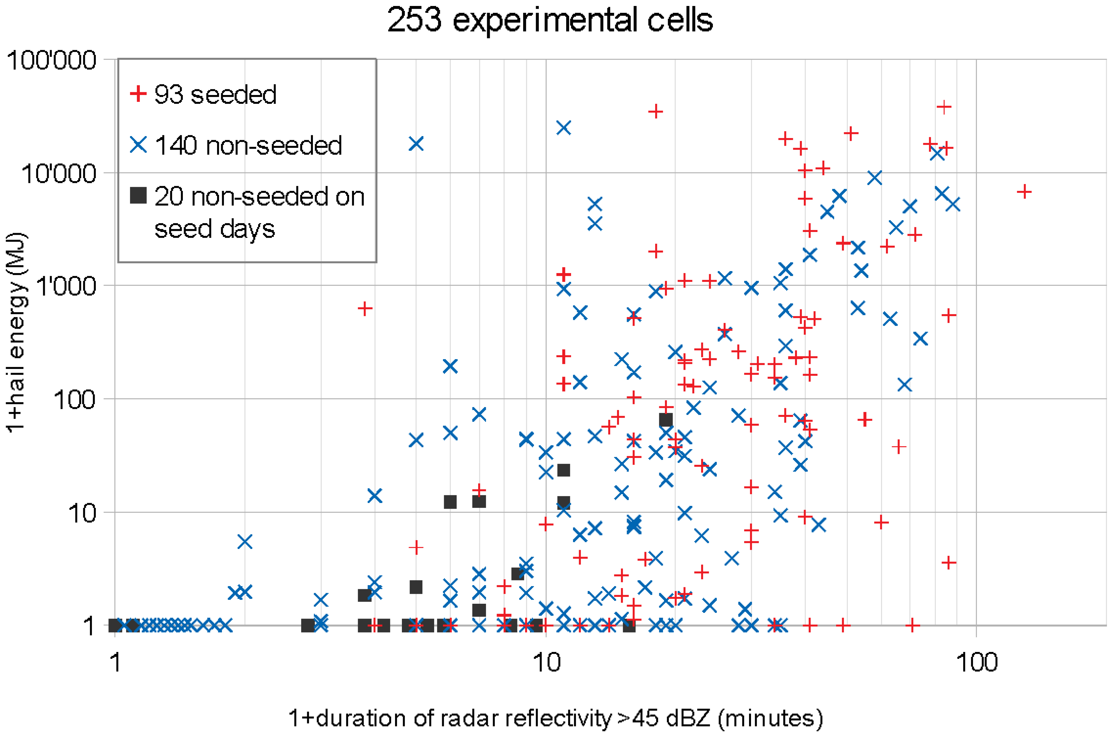
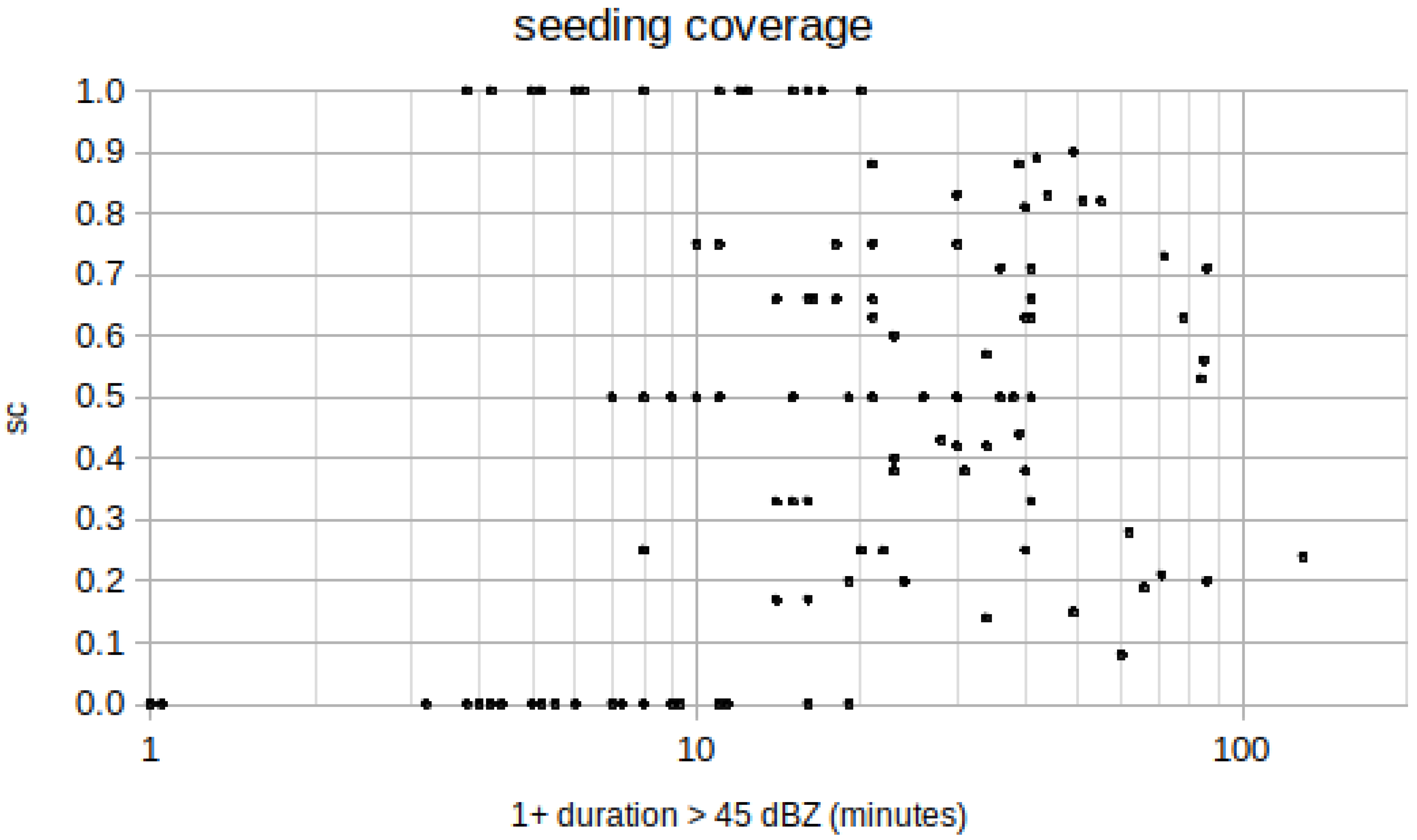
The present study is based on data found in the appendix of [7]: the hail energy on the ground $ln(E_{GR}+1)$, reconverted to $E_{GR}$, the seeding coverage $sc$, the beginning $t_0$ and the end $t_f$ of the seeding criterion met within the experimental area. The lifetime of a cell $t=t_f-t_0$ serves to stratify the data for figures or to convert $sc$ from cells to days. As randomization was done for days, the data given for cells had to be converted to the values relevant for the 83 experimental days. For the hail energy it is the sum of $E_{GR}$ for each day. For $sc$ the daily average is needed: $\sum (s{c}_i·t_i)/\sum t_i$. This is the really seeded fraction of the lifetime of all cells of a day.

We set the response variable $y=E_{GR}$ and the treatment variable $x=sc$. The sample size n is 253 cells or 83 days, whereas $n_s$ is the number of seeded cells (93) or the number of days with at least one seeded cell (34). Our interest is in a couple of parameters which characterize the difference $\mathit{dif}$ or the ratio $\mathit{rr}$ of y between seeded and non-seeded cells or days. There is a direct access from the variables y and x to the parameters $\mathit{dif}$ and $\mathit{rr}$ by the average of the non-seeded cells or days $\mathit{avn}$ and the weighted average of the seeded $\mathit{avs}$. Obviously the relation to the parameters is $\mathit{dif}=\mathit{avs}-\mathit{avn}$ and $\mathit{rr}=\mathit{avs}/\mathit{avn}$. The weighted seeded average $\mathit{avs}$ is calculated in this way:

$$\mathit{avs}=\frac{{\sum }_{i=1}^n(y_i·x_i)}{{\sum }_{i=1}^n{x}_i}$$

(2)

A practical, more or less self explaining code for such expressions is used in the free software “Octave”, compatible with Matlab: $\mathit{avs}=sum(y.\ast x)/sum\left(x\right)$, where .* indicates a term by term multiplication, and $\mathit{avn}=sum\left(y\right(x=0\left)\right)/length\left(x\right(x=0\left)\right)$.

When later permutations are applied on x to calculate probabilities, a problem could arise for the parameter $rr$ if $\mathit{avn}=0$. This could happen for certain permutations when there are less non-seeded cases than cases with no hail. However, this is not true for the hail data. Some hail is found within the non-seeded group for all permutations.

There is an elegant alternative to $\mathit{avn}$ and $\mathit{avs}$: correlation and regression. A classical measure of association between $E_{GR}$ and $sc$ is the Pearson correlation coefficient R, a versatile parameter. Two means as well as 2 × 2 contingency tables can be interpreted as a special case of correlation. R is standardized as a product of two “studentized” variables resulting in $-1\le R\le 1$.

$$R=\frac{1}{{\sigma }_y·{\sigma }_x}(-\overline{y}·\overline{x}+\frac{1}{n}\sum _{i=1}^n(y_i·x_i))$$

(3)

The sign of R is important. A negative sign points towards hail suppression and a positive sign towards increased hail energy when seeding. Correlation is the key to regression with a slope $R·{\sigma }_y/{\sigma }_x$ and an intercept $\overline{y}-\overline{x}·slope$, allowing to calculate alternative estimates of $\mathit{dif}$ and $\mathit{rr}$. The difference $\mathit{dif}$ is given in MJ per cell or per day, the ratio $\mathit{rr}$ is dimensionless (in 2 × 2 tables known as risk ratio). The difference $\mathit{dif}$ is just R multiplied by a constant:

$$\mathit{dif}=R·\frac{{\sigma }_y·\overline{x}·n}{{\sigma }_x·n_s}$$

(4)

The sample size n, the number of seeded cases $n_s=length\left(x(x>0)\right)$, the averages $\overline{y}$ and $\overline{x}$ as well as the std ${\sigma }_y$ and ${\sigma }_x$ do not change when x is permuted. Only the term ${\sum }_{i=1}^n(y_i·x_i)$ is affected by permutation.

More delicate is the formula for $\mathit{rr}=1+(\mathit{slope}·{\sum }_{i=1}^n{x}_i/n_s)/\mathit{intercept}$, because the intercept could become zero. This is explicitly shown in the following formula for $rr$:

$$\mathit{rr}=1+\frac{R·n/n_s}{-R+R_{cr}}$$

(5)

The critical constant $R_{cr}$ is

$$R_{cr}=\frac{\overline{y}·{\sigma }_x}{\overline{x}·{\sigma }_y}$$

(6)

$R_{cr}$ of the hail data is 0.44 and 0.66 for cells and days, respectively. These values are not changed by permutations. A second critical point $R_{c2}$ may be found at $rr=0$, corresponding to $R_{c2}=-Rcr·ns/(n-ns)$. When calculating probabilities for $\mathit{rr}$ by permutations or bootstrap, $R_i$ of every permutation i must be kept within these limits $R_{cr}$ and $R_{c2}$. This does not change the medians of R and $rr$ in the vicinity of $R=0$ or $rr=1$. Means, however, would be corrupted.

Table 1. Parameters $\mathit{dif}$ in MJ per cell and risk ratio $\mathit{rr}$ calculated by two models: regression or weighted average based on $\mathit{avs}$, $\mathit{avn}$. Conversion of $\mathit{dif}$ for days to MJ/cell by the factor 83/253. The probabilities calculated later in Section 3.2 are added.

Model	n	$\mathit{dif}(\mathbf{MJ}/\mathbf{Cell})$	$\mathit{P}\left(\mathit{dif}\right|{\mathit{H}}_0)$	$\mathit{rr}$	$\mathit{P}\left(\mathit{rr}\right|{\mathit{H}}_0)$
regression (days)	83	1612	0.38%	3.27	0.38%
regression (cells)	253	1583	0.38%	3.01	0.38%
$\mathit{avs}$, $\mathit{avn}$ (days)	83	1721	0.53%	3.01	0.87%
$\mathit{avs}$, $\mathit{avn}$ (cells)	253	1942	0.29%	3.50	0.31%

shows the agreement and differences when calculating $\mathit{d}if$ and $rr$ by regression or by weighted averages. Both take unsatisfactory seeding into account, but in a different manner. The weighted average $\mathit{avs}$ neglects practically all of y when the corresponding x is close to zero. Regression is not affected by this kind of discontinuity. Therefore differences between the models must be expected. Ideally, $rr$ should be equal for the 83 days and 253 cells, whereas $\mathit{dif}$ is made to become comparable by converting $\mathit{dif}$ per day to $\mathit{dif}$ per cell by the factor 83/253. Hail cells are more interesting than days because the hail energy of cells can be compared to cells elsewhere, whereas for days such a comparison makes less sense. Table 1 reveals quite a difference between the models and an appreciably better agreement between days and cells for regression. Therefore the model regression is preferable.

It is important to note that the direct way by $\mathit{avs}$ and $\mathit{avn}$ is identical to regression when $sc$ is simplified to a binary seeded, non-seeded. This advantage does not outweigh the loss of accuracy when discarding the detailed information contained in $sc$.

3.2. The Calculation of Probabilities

The crucial question concerns the probability $P\left(R\right|H_0)$. Could it be that the observed R, $\mathit{dif}$ or $\mathit{rr}$ would be due to chance? If this chance is below the classical 2.5% in one of the two tails, the null hypothesis $H_0$ is judged improbable. The task is to calculate the probability for the observed results assuming that $H_0$ is true. Different methods will be compared with respect to the parameter R. One of the oldest is based on student’s t or Fisher’s z. The latter is simpler and a close approximation to the probabilities obtained by t.

$$z=0.5·{(n-3)}^{-0.5}·ln\left(\right(1+R)/(1-R\left)\right)$$

(7)

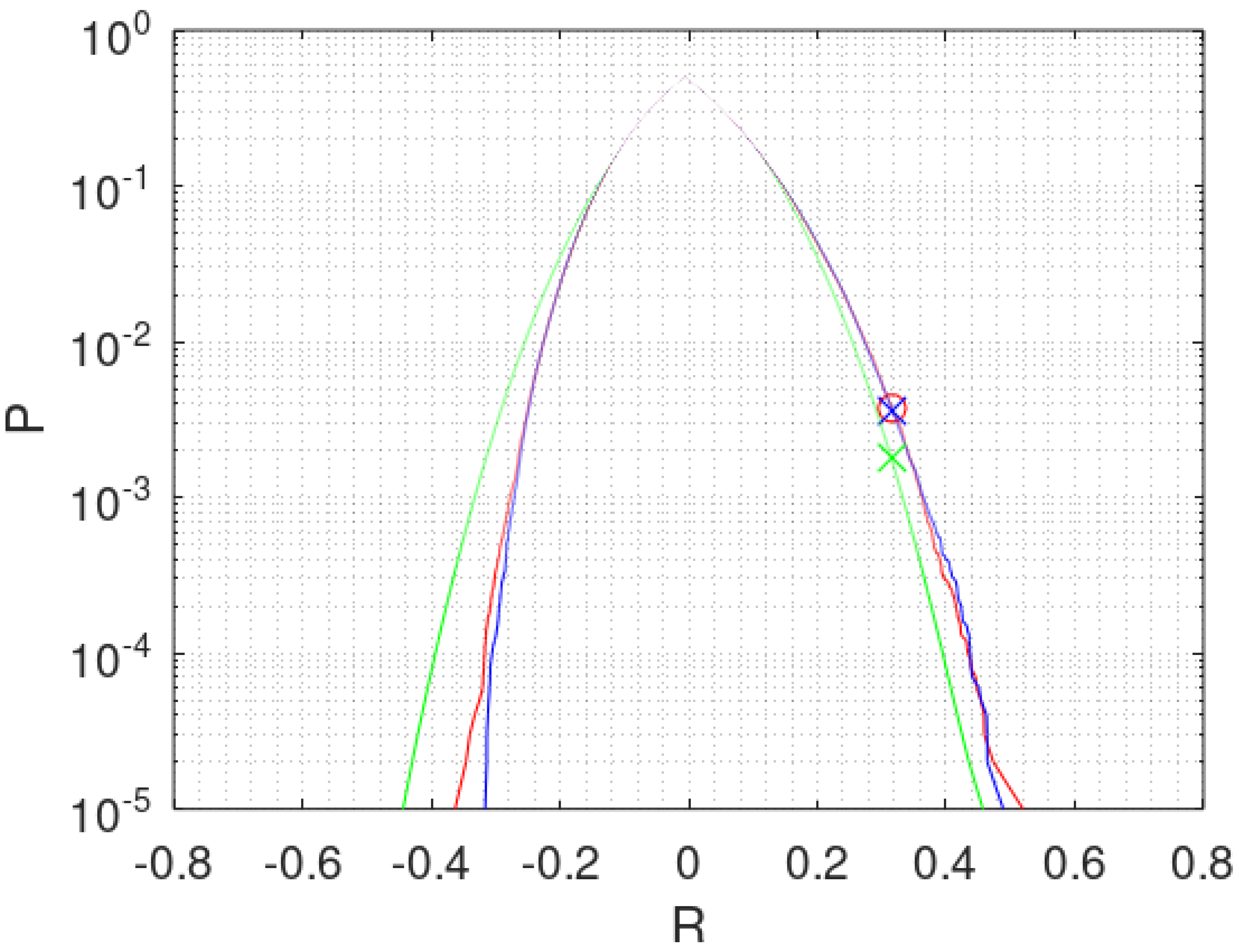
It should be noted that the original data $y=E_{GR}$ are not transformed, only R as part of the calculation of probability. If x and y are samples from normal distributions, z is a standard normal distribution. In this case $P\left(z\right)$ as well as $P\left(R\right)$ are known. The green line in Figure 3 shows the accumulated probabilities min$(P,1-P)$ for the 83 hail days starting from both extremes of R. This way of plotting a cumulated distribution function (cdf) allows to use a logarithmic scale with adequate resolution and showing both tails, peaking at the median of R.

The green curve for $P\left(R\right|H_0)$ is symmetrical, which is not realistic for the hail data. As the sample $E_{GR}$ is far from a normal distribution, combinative tests should be applied. The randomization test is such a test, characterized by the permutation of one variable. It was introduced by R. A. Fisher in 1924 according to [17] (p. 3). The confirmatory test of Grossversuch IV was a complicated version of the randomization test and regression in two dimensions [7]. It showed increased hail or whatever the logarithm meant, but did not reach statistical significance for several reasons already mentioned.

If $H_0$ is true, the relation between x and y is random and can be replaced by other random allocations of $x_i$ to $y_j$. This is systematically done by permutation of the scores in the samples x or y. Permutation changes only the covariance, the last expression in Equation (3), all other terms are preserved. This condition is called “fixed marginals” for binary samples expressed in a 2 × 2 table.

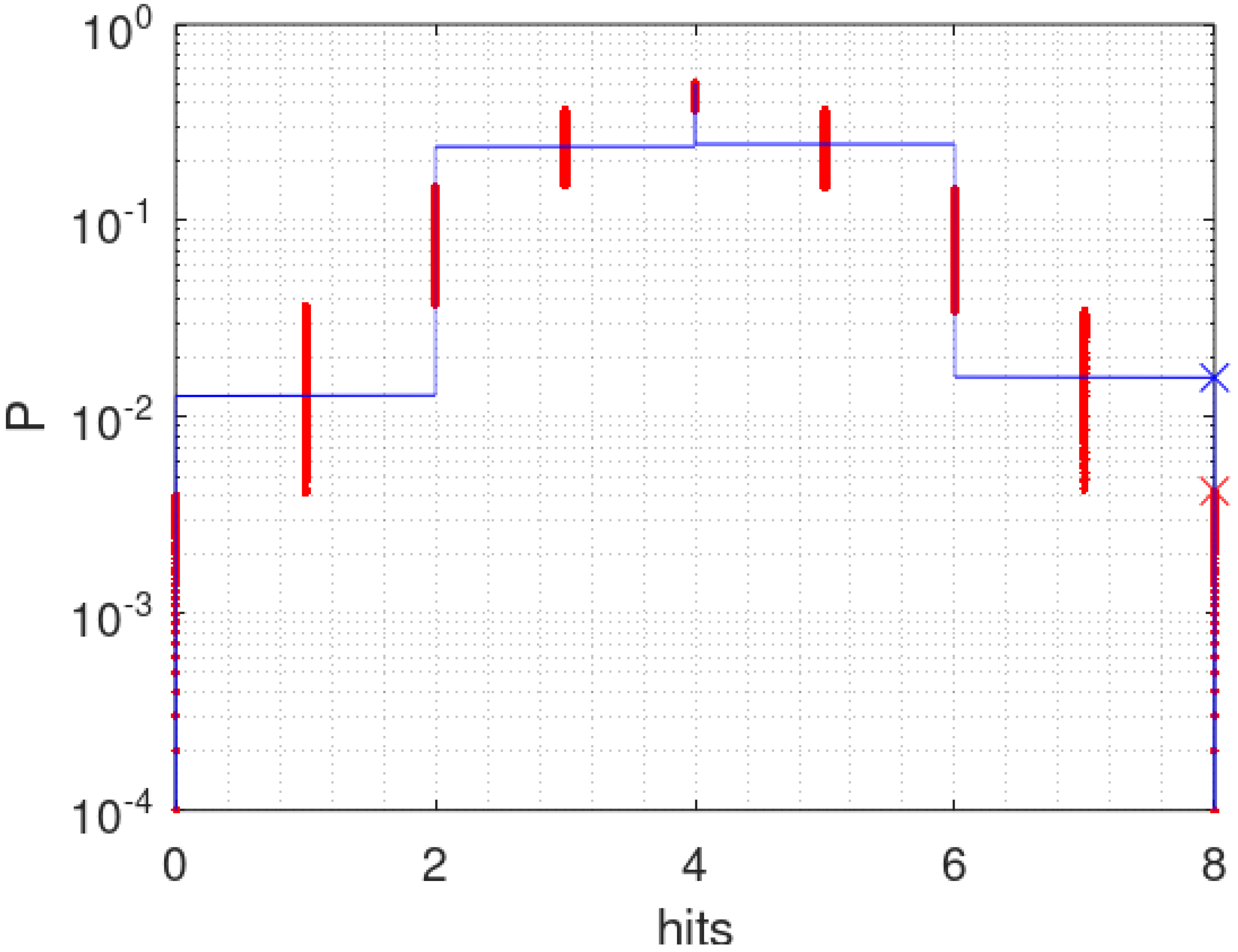
There are n! equally probable possibilities to rearrange the products $y_i·x_j$. If all permuted $R_i$ are sorted and plotted from both ends of smallest to larger and largest to smaller, a cdf of min$(P_i,1-P_i)$ is obtained. The endpoints of the cdf are the extreme correlations for both x and y sorted. The correlation between ascending x versus descending y gives the most negative or smallest $R_i$. Ties in x or y lead to repetitions of the same $R_i$ and the probability increases in steps of $1/n!$. We checked numerically that the complete permutation of small binomial samples $n\le 7$ arrives at probabilities which are $identical$ to Fisher’s exact solution for 2 × 2 tables.

In practice data of size $n!$ cannot be handled and the resolution 1/n! is not needed. Therefore the permutation distribution is approximated by N random samples. This is called resampling, rerandomization or Monte Carlo method. Such a plot starts and ends at $P=1/N$. The blue curve in Figure 3 shows the approximation by N = 100’000 points. Each permutation is represented by a point $R_i$. The points are sorted and connected to a line zigzagging from 0.001% to 0.002%, 0.003% and so forth. From 0.1% onward the curve becomes stable as may be seen.

The precision in terms of the std of P is given by

$${\sigma }_P={((P-P^2)/N)}^{0.5}$$

(8)

This is also found in [18] (p. 97). The resampling is done with replacement. The consequences of replacement are negligible in the context of permutations. It just means that the complete permutation distribution is never met exactly, even when N is equal or larger than $n!$, but the error is known.

Another combinative method to calculate probabilities is bootstrapping, mostly used for confidence intervals [11]. The bootstrap creates new samples by selecting n times from y, from x or from both, with replacement. In this way an association between y and x is also broken. Bootstrapping without replacement is like permuting. Bootstrapping with replacement creates new samples with different mean and std. We bootstrap y, the most critical distribution. The red curve in Figure 3 shows the result for applying bootstrap to $E_{GR}$ of the 83 hail days 100,000 times. The coincidence of the red curve with the blue curve from permutation is most remarkable. The probabilities $P\left(R\right|H_0)$ are 0.38% for both. Doing the same for the 253 cells shows also good coincidence (0.38% for permutation and 0.34% for bootstrap). The difference between permutation and bootstrap in Figure 3 is negligible. In certain conditions the differences could be considerable as explained in the Appendix A. However, in the case of the hail data, distributions and correlations are not sensitive to the model of calculation applied. Otherwise detailed knowledge of the experimental circumstances may have been necessary to chose the adequate model, if possible.

Calculations based on R and regression have a great advantage insofar as permutations form $R_i$, ${\mathit{dif}}_i$ and ${\mathit{rr}}_i$ in the same succession, leading to identical probabilities $P\left(R_i\right|H_0)$, $P\left({\mathit{dif}}_i\right|H_0)$ and $P\left({\mathit{rr}}_i\right|H_0)$. This is not the case for the seemingly simpler model using averages $\mathit{avs}$ and $\mathit{avn}$ instead of R and regression. Table 1 shows the differences.

From this point in the analysis the regression model is pursued. The other data in Table 1 are less compact, but all in a range of probabilities far below 2.5%. This is good evidence for a statistically significant correlation between $E_{GR}$ and $sc$ in the sense that the hail energy is increased when seeding.

3.3. Confidence Intervals and Standard Error

The next question is about the accuracy of R and the derived $\mathit{dif}$ and $\mathit{rr}$. Confidence intervals ($CI$) are the means to treat these issues. Resampled distributions with $R_i$ are needed assuming the alternative hypothesis $H_1$ that R found in the experiment is true and should correspond to the median of the resampled $R_i$. An old solution for normally distributed y and x is again Fisher’s z for $CI$.

$$z_i=0.5·{(n-3)}^{-0.5}·ln((1+R_i)·(1-R)/((1-R_i)·(1+R)))$$

(9)

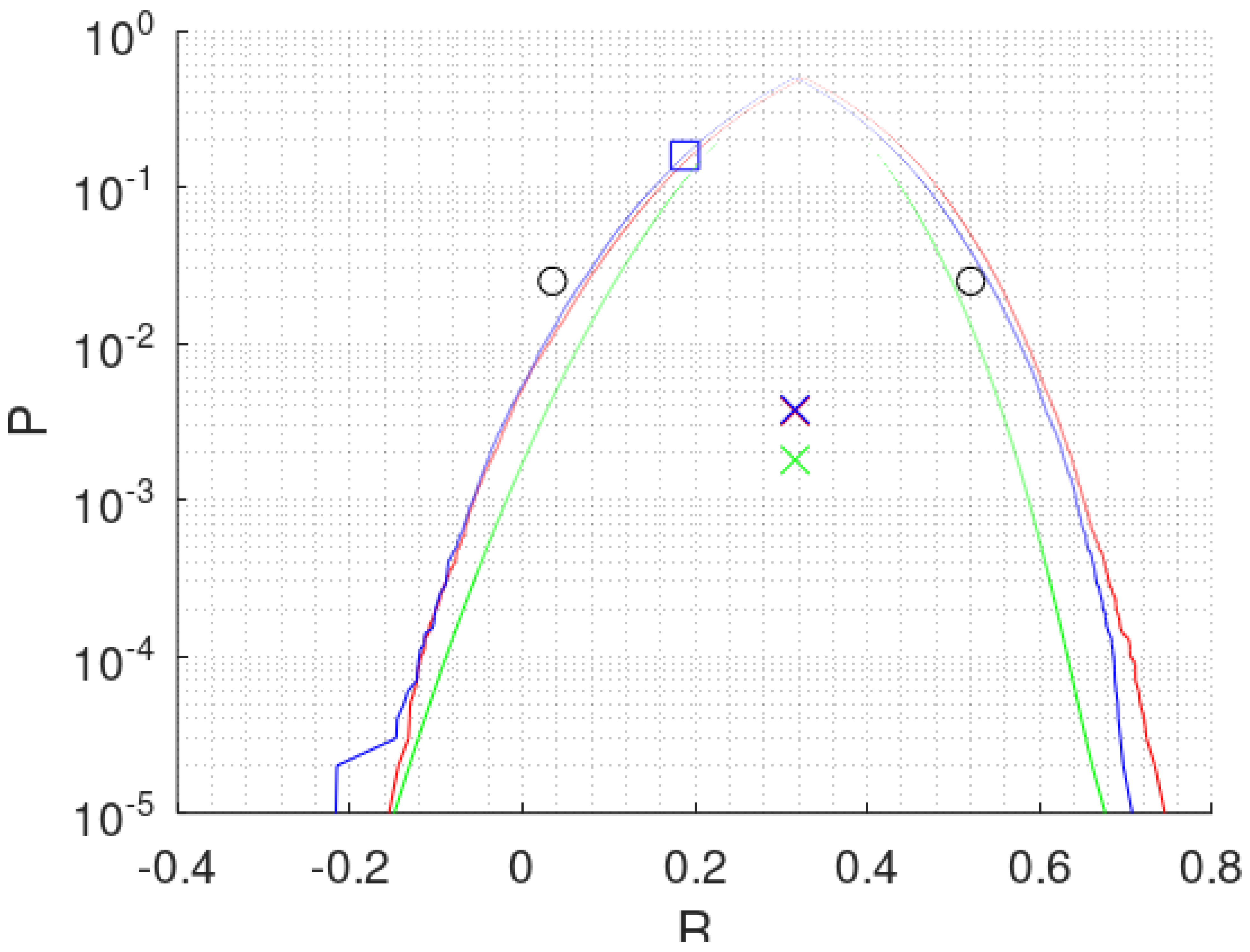
As above, a standard normal distribution with $z_i$ is expected when y and x are Gaussian. The green curve in Figure 4 is again shown for comparison with the solutions by combinative methods.

One such method is "bivariate" bootstrapping to calculate $CI$ by resampling the originally associated $x_i$ and $y_i$ pairwise with replacement. In this way the correlation of the sample is preserved in the average of all bootstraps producing $R_i$, although median$\left(R_i\right)=R$ is not guaranteed. Performing this bootstrap leads to the red curve in Figure 4.

Instead, permutation keeps all terms of y and x but varies the associations between, which destroys any correlation. In the course of this work, a simple and transparent way was found to impose the observed (or any other possible) R as the median of all permutations. After permutation, a random sequence of length $m_1$ is sorted to produce the maximum positive or, when R is negative, the maximum negative correlation. This $m_1$ is used to compensate, by construction, for the loss of correlation in the randomly permuted terms. The task is to find the correct $m_1$ which guarantees median$\left(R_i\right)=R$ (see Figure 4). An adequate $m_1$ to start with is:

$$m_1=R·(n-m_0)/R_{max}$$

(10)

The term $m_0$ is an optional number of randomly selected pairs keeping their original association (as with bivariate bootstrapping). The portion of the sample subjected to permutation is $n-m_0-m_1$. This procedure to resample $R_i$ by permuting and maximising the association of $m_1$ random terms may be named “correlation imposed permutation” (CIP). CIP keeps all terms of y and x and plays with the associations between y and x to form a permutation distribution for $CI$. There are $n!/(m_1!·m_0!)$ permutations, approximated by N scores $R_i$ as explained in Section 3.2.

Equation (10) situates the median of the permutations already in the vicinity of R. The correction to establish a better $m_1$ for the next approximation is (R-median$\left(R_i\right))·(n-m_0)/Rmax$. By two or three further runs median$\left(R_i\right)=R$ is reached with adequate precision.

Figure 4 shows the blue curve for CIP, n = 83 days, $m_0=0$, $m_1=32.7$. A non integer $m_1$ is needed for the accuracy of the condition median$\left(R_i\right)=R$. It is realized by alternating in the present case between 7 times $m_1=33$ and 3 times $m_1=32$. The blue curve in Figure 4 is close to the red curve as already found in Figure 3. Again, the hail data are indifferent with respect to the two models applied for calculation.

Concerning $m_0$ there is an interesting suggestion based on Equation (9): when using z, $P\left(R\right|H_0)$, indicated by a green cross in the middle of Figure 4, is identical to $P(R_i=0|H_1)$. As an option, this condition could be applied to determine $m_0$ in CIP. Increasing $m_0$ decreases slightly $CI$. Introducing $m_0=18$ for the 83 hail days or $m_0=96$ for the 253 hail cells complies with this option.

In Figure 4 the confidence interval $CI$ is the distance between the two tails of a curve at e.g., $P=2.5\%$. At this level the $CI$ is about four std (3.9 for normal distributions) and comprises 95% of all randomly resampled cases. Two black circles are noted outside the curves. They were calculated by the “bias corrected and accelerated” (BCa) bootstrap method going also back to Efron [19]. BCa is complicated and seems to us less convincing than the simple bootstrap or CIP. It was checked that CIP fits best Fisher’s z when the samples y and x are representative for normal distributions. A survey on bootstrapping dealing also with shortcomings is found in [10]. A further critical point mentioned by Cox [20] are samples that are too small to be representative for a parent distribution. The Appendix A deals with this problem.

Instead of reading the curves for $CI$ at 2.5% we prefer the blue square at a probability of 15.9% in Figure 4. The value of 15.9% corresponds to $R-\sigma$ in normal distributions. The standard error ($\sigma$) is an adequate measure of error. The interesting side is towards zero effect, therefore the parameters $\mathit{dif}-\sigma$ and $\mathit{rr}-\sigma$ will be shown in

Table 2. Results for hail data of Grossversuch IV.

Experiment	Unit	Seeded	Non-s.	$\mathit{dif}/\mathbf{cell}$	$\mathit{dif}-\mathit{\sigma }$	$\mathit{P}\left({\mathit{H}}_0\right)$	$\mathit{rr}$	$\mathit{rr}-\mathit{\sigma }$
$E_{GR}$ versus $sc$	days	34	49	1612	966	0.4%	3.3	2.1
$E_{GR}$ versus $sc$	cells	93	160	1583	880	0.4%	3.0	1.8
Means of two groups
$E_{GR}$ versus seeded, non-seeded	days	34	49	1316	665	2.0%	2.6	1.6
$E_{GR}$ versus seeded, non-seeded	cells	93	160	1615	964	0.5%	3.1	2.0
Two groups (for comparison to [7]: cells planned for seeding but not seeded are attributed to seeded group)
$E_{GR}$ versus planned, non-planned	cells	113	140			3.7%	2.2	1.4
Federer [7] Table 21, $C\left(\alpha \right)$ test	cells	113	140			1.9%	2.2	1.5
$2\times 2$ contingency table
hail, no-hail versus seeded, non-seeded	cells	78 + 15	111 + 49			0.5%	1.2	1.1
idem, for hailpads (213 cases)	cells	45 + 29	64 + 75			2.1%	1.3	1.2

. The other side of the 15.9% probability is asymmetric and vulnerable with respect to the parameter $rr$. The influence of a nearby singularity at $R_{cr}$ may distort the cdf (see Equation (6)).

3.4. Re-Evaluated Results of Grossversuch IV

The most important results of the statistical evaluations are found in Table 1 and in Figure 3 and Figure 4. The following Table 2 provides some further insight. It starts with the results of the regression model in rows 1 and 2, continuing with a binary x reducing $sc$ to 0 or 1 in order to compare the present evaluations with results presented in 1986 [7].

Statistical significance is best in rows 1 and 2 because the information contained in $sc$ is used. The bold scores show the most reliable results. Looking at cells is closer to the question asked, but the randomization was done for days. Therefore $P\left(H_0\right)$ earns more credit when calculated for days. The difference between the evaluation of $P\left(H_0\right)$ in row 1 and 2 of Table 2 is astonishingly small in view of the big difference of n. The aggregation of data from cells to days reduces stochastic variations as well as skewness and kurtosis.

In rows 3 and 4 of Table 2 most information with respect to unsatisfactory seeding is lost. A big misinterpretation happens for row 3 because 17 non-seeded cells are taken into account as seeded in the seeded days. Only 3 cells occurring alone on 3 seeded days shift to non-seeded. Correspondingly $P\left(H_0\right)$ jumps to 2.0%. The loss in row 4 is less severe because 20 cases of planned but not performed seeding are transferred to non-seeded. Therefore the influence on $P\left(H_0\right)$ is not dramatic.

To allow a comparison with the results of Table 21 (last row) in [7], all 20 non-seeded cells on planned seed days were taken as perfectly seeded in rows 5 and 6. This merging of data causes a distortion that leads to the loss of statistical significance in our evaluation. By the way, the $C\left(\alpha \right)$-test used in [7] (p. 945) is not adequate. It can reveal a constant multiplicative seeding effect, but this implies that the distributions of the seeded and non-seeded $E_{GR}$ may differ by scale but not by shape. The skewness and kurtosis are kinds of shape parameters. For the seeded and non-seeded (in parentheses) cells, 3.6 (5.8) is found for the skewness, 16.3 (40) for the kurtosis. This does not look good enough for a $C\left(\alpha \right)$-test, the randomization test must be preferred.

Row 7 shows that the probability for a cell to produce hail is significantly increased by some 20% when seeding. The data from hailpads (row 8) confirm this finding, but the significance becomes marginal because of reasons discussed later. For rows 7 and 8 the results of bootstrapping were chosen because the fixed marginals anticipated by permutation are not adequate here and the differences in 2 × 2 tables notable: $P\left(H_0\right)$ = 0.7% and 2.8% would be obtained. A more impressive example is discussed in the Appendix A.

To sum up Table 2: Seeding increased the hail energy by a factor of 3, the difference with respect to non-seeded was about 1600 MJ per cell and the chance to obtain this result accidentally was 0.4%, therefore statistically significant. The results hold for an average seeding of $\overline{sc}=0.48$. An extrapolation to perfect seeding is not recommended.

Not included in Table 2 are some further evaluations performed with cleaned up sets of data: either 118 cells of lifetimes less than 15 min for the 45 dBZ contour, or 39 cells with unsatisfactory seeding ($sc<1/3$) could be excluded. The latter was planned in the original design of Grossversuch IV (see [7] (p. 925)). The first 4 rows of Table 2 were combined with one or both of these exclusions yielding 12 further evaluations. There is always an increase for seeding, all at a significance level below or close to 2.5%. A trend to still lower $P\left(H_0\right)$ than in Table 2 was observed when excluding cells of short duration. All these different evaluations and models form a homogeneous picture. Even the linear regression associated with $sc$ may be changed to a power p within $0<p<1.5$. The homogeneous picture does not change. Powers p much larger than 1 do not make sense. A power very close to zero leads to the binary simplification seeded or non-seeded.

The preparation of the data and the evaluations are easily performed using the spreadsheet “DataHail-FMA” available in the Supplementary Materials. The evaluation of $P\left(R\right|H_0)$ in the spreadsheet is based on the first four moments of the permutation distribution, a method proposed by Pitman [21]. This procedure is less robust than permutations or bootstrapping but quick and precise for the hail data. The spreadsheet contains also the calculations concerning autocorrelation, which is the next issue.

Federer [7] (p. 929) observed a weak intra-day correlation, amounting to 0.33 for $ln(E_{GR}+1)$. For non-transformed $E_{GR}$ and non-seeded cells we found a lag-1 intra-day autocorrelation of R = 0.47 at $P\left(H_0\right)$ = 1.0%. For cells on seeded days the autocorrelation disappears: $R=-0.05$ at $P\left(H_0\right)$ = 44%. As $E_{GR}$ changes under the influence of a varying $sc$, the autocorrelation is destroyed. R, $\mathit{dif}$ or $\mathit{rr}$ are not affected by the autocorrelation, only the calculation of $P\left(H_0\right)$ may be too optimistic when the independence of the units is not perfect. The following experiment localizes the effect of autocorrelation on $P\left(H_0\right)$.

The distribution of $E_{GR}$ with cells is varied in the set of non-seeded data, while the daily total of $E_{GR}$ remains unchanged. The two most extreme cases are:

• Each cell contributes the same amount to the daily $E_{GR}$ of non-seeded cells, corresponding to total intraday autocorrelation. The result of the permutation test for the 253 cells is $\mathit{rr}$ = 3.0, $P\left(H_0\right)$ = 0.27%.
• The daily total comes from only one cell, the other cells of the same day are without hail. In this case $\mathit{rr}$ = 3.0, $P\left(H_0\right)$ = 0.74% is obtained.

In this bandwidth from 0.27% to 0.74% the observed result is found: $\mathit{rr}$ = 3.0, $P\left(H_0\right)$ = 0.38%, equal to the result for days ($\mathit{rr}$ = 3.3, $P\left(H_0\right)$ = 0.38%). It seems that the intraday autocorrelation of non-seeded cells is not really disturbing. Also Federer Table 22 [7] based 16 of their 21 tests on cells. Autocorrelation could have been a real problem if the several severe hailstorms would have been aggregated on a few days. However, there is only one day, 18 July 1978, non-seeded, with two very large cells, causing the daily maximum of $E_{GR}={43}^{\prime }000$ MJ. A plausible explanation of the autocorrelation is the aggregation of cases with zero or little hail on days with meteorological conditions not suitable to produce severe storms.

Autocorrelation is not observed in the data from hailpads. This has to do with an interesting question: how do stochastic uncertainties in the measurements influence the results? From [13,14] we estimate the uncertainty of the radar based $E_{GR}$ within 25%. In case of a systematic multiplicative error in the radar calibration and thus in $E_{GR}$, the significance level $P\left(H_0\right)$ remains unchanged. The reason is that linear transformations do not change R. If the error in $E_{GR}$ is stochastic, it has an impact on $P\left(H_0\right)$, as a simple numerical test can show. We added a random error of 20% to $E_{GR}$ of unit days, first row in Table 2, repeating the experiment 100 times. The significance level diminishes as $P\left(H_0\right)$ increases from 0.33% to an average of 0.55%. When increasing the error to 40%, there is a further impairment of $P\left(H_0\right)$ to 1.1%. In both cases $\mathit{rr}$ remains practically unchanged and $P\left(H_0\right)$ remains below 2.5%.

We learn from this that data suffering from too much inaccuracy lose power. Unfortunately, this seems to be the case for the data obtained from hailpads. Also the hailpad data show an increase of hail energy for seeded data, but statistical significance is not reached, e. g. for cells $\mathit{rr}$ = 1.58, $P\left(H_0\right)$ = 16%. Federer’s Table 21 [7] reports $\mathit{rr}$ = 1.58, $P\left(H_0\right)$ = 24% for the $C\left(\alpha \right)$ test. The data from hailpads lack 40 cells mainly from the year 1982. However, this can not be the decisive point, as the radar data reach for the same 213 cells still $\mathit{rr}$ = 2.79, $P\left(H_0\right)$ = 0.7%. We suspect that the sampling by hailpads introduces intolerable stochastic variations. This hypothesis was tested by looking at the intraday autocorrelation of the hail energies from hailpads for unseeded days. Comparing the radar data for the same 79 cells to the hailpad data reveals R = 0.47, $P\left(H_0\right)$ = 1.2% for the radar, degrading to R = 0.09, $P\left(H_0\right)$ = 16% for the hailpads. This is a strong hint that the accuracy of the hailpad measurements is not adequate to show the intraday autocorrelation. Furthermore, the total hail energy is 0.41 times that of the corresponding $E_{GR}$. The conjecture is that the hailpad network not only introduces large stochastic errors but causes a loss of information which is important for the evaluation of hail energies. Less demanding is the question whether at least one hailpad was hit, indicating hail or no hail. Again, the hailpads identified less hail (51%) than the radar (75%) for both seeded and non-seeded experimental cells.

4. Discussion

4.1. What Transformations Do

We criticized the 1986 evaluation of Grossversuch IV in [7] on behalf of the logarithmic transformation of the hail energy $E_{GR}$. However, something positive about it was already mentioned: As the influence of a few dominating cases is transformed away by the logarithm, the chance is increased to find a significant correlation between $ln(1+E_{GR})$ and $sc$ or its binary transformation. Indeed this correlation is positive at a level $P\left(H_0\right)$ = 0.008% for $sc$ and 0.006% for the binary $x=0$ or 1. This may help to rule out $H_0$ and confirm the result that seeding increased hail.

It could have been quite different. We give an example which leads to the situation of a positive correlation for $E_{GR}$ and a negative correlation for $ln(1+E_{GR})$, both at very low levels of $P\left(H_0\right)$. A simple synthetic example works with three different values of $E_{GR}$ and $ln(1+E_{GR})$, respectively:

• 100 seeded and 20 non-seeded cells with both $E_{GR}$ and $ln(1+E_{GR})$ = 0
• 100 non-seeded cells with $E_{GR}$ =150, $ln(1+E_{GR})$ = 5
• 20 seeded cells with $E_{GR}$ = 3000, $ln(1+E_{GR})$ = 8

For $E_{GR}$ the correlation is positive, $P\left(H_0\right)$ = 0.01%, $\mathit{rr}$ = 4.0. For $ln(1+E_{GR})$ the correlation is negative, $P\left(H_0\right)\ll 0.001\%$, $\mathit{rr}$ = 0.32. A Wilcoxon-test where the data are filled into three ranks 0, 1 and 2 yields also a negative correlation, $P\left(H_0\right)\ll$ 0.001%, $\mathit{rr}$ = 0.40. These two transformations invert a statistically significant result to the opposite with even stronger significance. This example is a simplified version of what happens if seeding would prevent hail in small storms and enhance hail growth in a few very large storms. This scenario is not unrealistic and, if it should happen, hard to prove. In fact, the data of Grossversuch IV are close to this pattern, but only the increase of $E_{GR}$ for seeded storms reach statistical significance.

It is interesting to see how the results of the 1986 study react on transformations to the logarithm or to ranks (WMW-test, after Wilcoxon, Mann and Whitney). Without transformation we find always $rr>1$, namely $1.26<rr<4.38$ (see Table 22 [7]). The transformations produce both $\mathit{rr}>$ 1 and more often $\mathit{rr}<$ 1. The latter reminds our synthetic example above. Our study does not speak against hail suppression in short lived cells (life time less than 15 min of radar reflectivity >45 dBZ). We find $\mathit{rr}<$ 1, but this could be real as well as accidental.

The point is that the parameters R, $\mathit{dif}$ or $\mathit{rr}$ should be calculated using the variables y and x describing the issue (see [22] or [23] (p. 246 ff)). Nonlinear transformations of x or y lead away from what was asked. This criticism holds also for the transformation to ranks. Non linear transformations change R, $\mathit{dif}$ and $\mathit{rr}$ as well as $P\left(H_0\right)$. Something else is transforming R to Student’s t or Fisher’s z. This is just changing the functions to calculate the probability (which for non-normal data is no more a t or a normal distribution as permutations show). The condition is, that sorting $R_i$ or sorting a transformation of $R_i$ keep the same sequence when using permutations.

4.2. Multiplicity Effects

The authors of the 1986 paper state about the unfavorable seeding effect shown in their Table 21, that statistical significance “may easily be attributed to the multiplicity effect (which means that some out of a number of tests turn out significant by pure chance), but seeding influences are also a possible explanation” [7] (p. 949).

The question of the study was formulated as follows [7] (p. 923): “Do the experimental cells on seed days and no-seed days differ in the response variable in a statistically significant way?” As this question allows for either increasing or decreasing effects of seeding on hail formation, the significance level of the usual 5% is split into 2.5% for positive and 2.5% for negative influence. The planned evaluation of $ln(E_{GR}+1)-f$ in [7] missed the goal of finding out whether seeding had a statistically significant effect on the hail energy. The logarithmic a posteriori predictor f added a disturbing complexity and inaccuracies. In fact the average hail energy of the 113 planned non-seeded controls was only 20% of what $exp\left(f\right)-1$ would have predicted (61% for f). The present analysis remains as close as possible to the original question of the study and keeps the hail energy $E_{GR}$ as response variable. Furthermore, it makes use of the information on rudimentary seeding or non-seeding when seeding was planned. The permutation test of the correlation between $E_{GR}$ and $sc$ in agreement with the bootstrap is the most adequate mathematical treatment for the question asked. Therefore, it earns due credit and does not fall into the category where “multiplicity effect” [7] (p. 949) could happen.

The multiplicity effect comes into play when new questions diverging from $E_{GR}$ versus $sc$ are asked, e.g., about the duration t of the radar reflectivity >45 dBZ. There is undoubtedly a correlation between $E_{GR}$ and t: $R=0.37$, $P\left(H_0\right)=0.001\%$. This can not be accidential, $P\left(H_0\right)$ is definitely too low. However, how seeding influences the duration is statistically less certain. For t versus $sc$ the result is $R=0.16$, $P\left(H_0\right)=0.7\%$. Regression yields for t$\mathit{dif}=6$ min, $rr=1.3$. The credibility of such results is a delicate matter because it depends on how many questions were asked. Also those not reported should be counted.

4.3. Possible Mechanisms

Theories or modelling of the cloud physical processes increasing the hail energy of seeded storms are outside the goal of this paper. However, some ideas are put forward to show that the observed result is plausible. The formation of hail in a thunderstorm is a fortuitous matter. Ice and super-cooled water are necessary as well as updrafts matching the fall-speed of hailstones, keeping them half an hour in zones of super-cooled water and enabling several ups and downs. Complicated non-linear processes are involved which implies high sensitivity to small differences in the initial state of the atmosphere. No wonder that the prediction of hail energy is difficult. Seeding with silver iodide triggers freezing of supercooled water at temperatures up to −5 degrees Celsius. This may reduce hail due to competition, but, it may as well enable new scenarios for the formation of hail that would not have been possible without seeding.

Hail forms when super-cooled liquid water is captured by ice particles and then freezes on the surface. The processes and variables involved are complex (see for instance [24,25,26]). The primary material for growth is super-cooled water present in the form of droplets. We can distinguish between two scenarios depending on the balance between the amount of super-cooled water and the number of ice particles including hail embryos and hailstones.

In the first scenario, super-cooled water is abundant, even after seeding, and there are not enough ice particles to deplete the supercooled water substantially. Seeding will create ice crystals and increase their number in zones up to −5 C, leading to more hail embryos also in places where otherwise no ice would have been generated by natural ice forming nuclei. This gives way to more intensive as well as new scenarios of hail growth starting in relatively warm zones. Given abundant supercooled water, this forms the basis for the growth of additional and larger hailstones. Without sufficient competition, the opposite happens of what seeding is supposed to do.

In the second scenario there is a shortage of super-cooled water in relation to the number of ice particles. By increasing the number of freezing nuclei seeding will enhance competition among embryos. This may inhibit the growth of large hailstones, which is the underlying assumption of hail suppression by seeding.

The results presented in this study, however, suggest that the first scenario is dominating, at least for the severe storms which add up to a large part of the total hail energy. This is supported by recent findings that dry growth is unimportant for large hail [25]. Examples for large hailstones indicating wet growth are given in [27]. Another example is the 766 g hailstone of Coffeyville (NCAR Fact Sheet, October 1970) with typical protrusions indicating wet growth. These examples stand for severe storms with plenty of super-cooled water. It is doubtful whether seeding can reduce the amount of super-cooled water adequately. In any case, some of the extra ice particles produced by seeding may stick to the wet surface of growing hailstones, which would enhance growth and counteract the competition theory of seeding. These are plausible explanations of how seeding could enhance hail.

Last but not least, an increase of the number of hail-cells was found when seeding: $\mathit{rr}$ = 1.2, $P\left(H_0\right)$ = 0.5% and 0.7% for bootstrap and permutation, respectively. When looking at the days as unit no such increase is observed. The interpretation is that some experimental days offered just unsuitable conditions for hail, whether seeded or not. The observed intra-day autocorrelation supports this suggestion. On the other hand, the triggering of supplementary hail cells by seeding on days that have already produced hail can not be detected when analyzing days.

A last question concerns the factor of 3 found for the increase of hail energy when seeding. It seems large. Is it due to more or larger hailstones? A relatively modest factor of 1.2 can be attributed to an increased probability that seeded cells produce hail, as documented in Table 2, row 7 and 8. More important is the factor of 1.8 found by Federer et al. [7] Table 13 for an increase of the area touched by hail when seeding was planned (two-sided $P\left(H_0\right)$ = 2.9%, $C\left(\alpha \right)$-test). Most probably the factor 1.8 underestimates the reality because $sc$ was replaced by what was planned. We expect that an analysis using $sc$ would show an increase somewhere between 2 and 3, as well as better statistical significance, similar to the differences found for $E_{GR}$ in Table 2, comparing row 2 with row 5. Unfortunately, the data of the hailed area are not found for the individual cells in [7]. Anyhow, the statistical treatment of the question concerning the area is the least demanding because it boils down to the number of hailpads touched by hail. In this respect, the density of the network may yield sufficient resolution.

Maybe that seeding creates also some situations favourable to grow larger hailstones. The 30% longer duration of the 45 dBZ radar contour points to this possibility (see end of Section 4.2). The mentioned average of $\mathit{dif}=6$ minutes would be enough time to account for a threefold increase of kinetic energy. As the energy $E_{GR}$ is proportional to $D^4$, a small difference of hailstone diameter has a large impact on hail energy. On the other hand, the size of the largest hailstones depends on the updraft velocity which is governed by the dynamics of the storms. The latter may be influenced by the latent heat of freezing, which is liberated at warmer temperatures when seeding.

The considerably increased area of hail, the increased probability for hail and the longer duration of the cells sustain the idea that seeding enables additional hail scenarios.

5. Conclusions

The conclusion of the present re-evaluation is, that the seeding in Grossversuch IV increased the hail energy by $\mathit{dif}$ = 1600 MJ/cell, which is a factor of $rr=3$. This pertains to an average seeding of $\overline{sc}=0.48$. The precision is rather marginal, $rr=2$ is within one std. However, the statistical significance is almost sure, as all evaluations yield $P\left(H_0\right)$ below 2.5% and these using the full information contained in $sc$ are nearly an order of magnitude below 2.5% (see Table 2, row 1 and 2).

From a physical point of view, the result is not unrealistic, although a model proving that it must be so can not be given at this time. Most likely, seeding enhances further scenarios of hail production starting at warmer temperatures, increasing the area of hailfall by about a factor of 2, augmenting the occurrence of hail by some 20% and extending the duration of the 45 dBZ radar echo by about 30%. However, the multiplicity effect and marginal statistical significance cast uncertainty on these exploratory results.

Stochastic variations reduce statistical significance. The hailpad network, although it was one of the most dense and expensive we know of, was not good enough to measure reliably the total hail energy. At least it revealed that the area touched by hail when seeding was enlarged by a factor of 1.8 according to [7] and even more when some inaccuracy concerning the seeding is removed.

The statistical evaluation required much space because the 1986 study [7] was not satisfactory in this respect and some problems associated with asymmetric or heavy tailed distributions as well as non representative samples are still a challenge. To go round these problems by applying non-linear transformations to the raw data such as a logarithmic transformation or a conversion to ranks inserts a distortion between the question and the answer. This was disturbing in the original evaluation of Grossversuch IV.

Statistical models are needed to calculate probabilities. Difficulties may arise from more or less clear assumptions underlying a model. Permutation and bootstrap used here are quite transparent. However, sometimes the data alone are not sufficient to find the correct probabilities as in the contingency table $\left|\begin{array}{cc}6& 0\\ 0& 2\end{array}\right|$ when the condition of fixed marginals is not correct (see Appendix A).

The sample size n divided by the kurtosis of the sample is an indicator of the effective sample size. If not much larger than 1 it is indicative of an outlier problem leading to differences between permutation and bootstrap as explained in the Appendix A. It is recommended to calculate $P\left(H_0\right)$ by permutation as well as by bootstrap. If there is agreement, the sample is indifferent with respect to these models. The continuation may be permutation and regression which offers a compact solution for the parameters R, $\mathit{dif}$ and $rr$. The present work opened up a way to evaluate also $CI$ by permutation CIP. This deserves further attention.

Finally it should be noted that the presented results are valid only for the thunderstorms and the seeding procedures of Grossversuch IV.

References

1. Rauber, R.M.; Geerts, B.; Xue, L.; French, J.; Friedrich, K.; Rasmussen, R.M.; Tessendorf, S.A.; Blestrud, D.R.; Kunkel, M.L.; Parkinson, S. Wintertime orographic cloud seeding—A review. J. Appl. Meteorol. Climatol. 2019, 58, 2117–2140. [Google Scholar] [CrossRef]
2. Sulakvelidze, G.K.; Kiziriya, B.I.; Tsykunov, V.V. Progress of Hail Suppression Work in the USSR. In Weather and Climate Modification; Hess, W.N., Ed.; Wiley: Hoboken, NJ, USA, 1974; pp. 410–431. [Google Scholar]
3. Rivera, J.A.; Otero, F.; Tamayo, E.N.; Silva, M. Sixty Years of Hail Suppression Activities in Mendoza, Argentina: Uncertainties, Gaps in Knowledge and Future Perspectives. Front. Environ. Sci. 2020, 8, 45. [Google Scholar] [CrossRef]
4. Abshaev, M.T.; Sulakvelidze, R.M.; Burtsev, I.I.; Fedchenko, L.M.; Jekamuklov, M.K.; Tebuev, A.D.; Nesmeyanov, P.V.; Shakirov, I.N.; Shevala, G.F. Development of Rocket and Artillery Technology for Hail Suppression. 2006. Available online: https://www.researchgate.net/publication/343691402_ACHIEVEMENTS_IN_WEATHER_MODIFICATION_-_UAE_PRIZE_FOR_WEATHER_MODIFICATION_Article_Development_of_Rocket_and_Artillery_Technology_for_Hail_Suppression_Copyrights_C_Department_Atmospheric_Studies_Minist (accessed on 28 November 2021).
5. Browning, K.; Foote, G.B. Airflow and hail growth in supercell storms and some implications for hail suppression. Q. J. R. Meteorol. Soc. 1976, 102, 499–533. [Google Scholar] [CrossRef]
6. Wieringa, J.; Holleman, I. If cannons cannot fight hail, what else? Meteor. Z. 2006, 15, 659–669. [Google Scholar] [CrossRef]
7. Federer, B.; Waldvogel, A.; Schmid, W.; Schiesser, H.H.; Hampel, F.; Schweingruber, M.; Stahel, W.; Bader, J.; Mezeix, J.F.; Doras, N.; et al. Main results of Grossversuch IV. J. Appl. Meteor. Climatol. 1986, 25, 917–957. [Google Scholar] [CrossRef] [Green Version]
8. Foote, G.B.; Knight, C.A. Results of a randomized hail suppression experiment in Northern Colorado. Part I: Design and Conduct of the experiment. J. Appl. Meteorol. 1979, 18, 1526–1537. [Google Scholar] [CrossRef] [Green Version]
9. Foote, G.B.; Wade, C.G.; Fankhauser, P.W.; Summers, P.W.; Crow, E.L.; Solak, M.E. Results of a randomized hail suppression experiment in Northern Colorado. Part IIV: Seeding logistics and post hoc stratification by seeding coverage. J. Appl. Meteorol. 1979, 18, 1601–1617. [Google Scholar] [CrossRef] [Green Version]
10. Bishara, A.J.; Hittner, J.B. Confidence intervals for correlations when data are not normal. Behav. Res. Meth. 2017, 49, 294–309. [Google Scholar] [CrossRef] [Green Version]
11. Efron, B. Bootstrap methods: Another look at the jackknive. Ann. Stat. 1979, 7, 1–26. [Google Scholar] [CrossRef]
12. Federer, B.; Waldvogel, A.; Schmid, W.; Hampel, F.; Rosini, E.; Vento, D.; Admirat, P.; Mezeix, J.F. Plan for the Swiss randomized hail suppression experiment. Design of Grossversuch IV. Pure Appl. Geophys. 1978, 117, 548–571. [Google Scholar] [CrossRef]
13. Waldvogel, A.; Schmid, W.; Federer, B. The Kinetic Energy of Hailfalls. Part I: Hailstone spectra. J. Appl. Meteorol. 1978, 17, 515–520. [Google Scholar] [CrossRef] [Green Version]
14. Waldvogel, A.; Federer, B.; Schmid, W.; Mezeix, J.F. The Kinetic Energy of Hailfalls. Part II: Radar and Hailpads. J. Appl. Meteorol. 1978, 17, 1680–1693. [Google Scholar] [CrossRef]
15. Waldvogel, A.; Schmid, W. The Kinetic Energy of Hailfalls. Part III: Sampling Errors Inferred from Radar Data. J. Appl. Meteorol. 1982, 21, 1228–1238. [Google Scholar] [CrossRef] [Green Version]
16. Schmid, W.; Schiesser, H.H.; Waldvogel, A. The Kinetic Energy of Hailfalls. Part IV: Patterns of Hailpad and Radar Data. J. Appl. Meteorol. 1992, 31, 1165–1178. [Google Scholar] [CrossRef] [Green Version]
17. Berry, K.J.; Mielke, P.W., Jr.; Mielke, H.W. The Fisher-Pitman permutation test: An attractive alternative to the F test. Psychol. Rep. 2002, 90, 495–502. [Google Scholar] [CrossRef] [PubMed]
18. Lee, W.C.; Rodgers, J.L. Bootstrapping correlation coefficients using univariate and bivariate sampling. Psychol. Methods 1998, 3, 91–103. [Google Scholar] [CrossRef]
19. DiCiccio, T.J.; Efron, B. Bootstrap confidence intervals. Stat. Sci. 1996, 3, 189–228. [Google Scholar] [CrossRef]
20. Cox, N.J. Speaking Stata: The limits of sample skewness and kurtosis. Stata J. 2010, 10, 482–495. [Google Scholar] [CrossRef] [Green Version]
21. Pitman, E.J.G. Significance tests which may be applied to samples from any populations. II. The correlation coefficient test. J. Roy. Stat. Soc. Suppl. 1937, 4, 225–232. [Google Scholar] [CrossRef]
22. Feinstein, A.R. Clinical Biostatistics XXIII: The role of randomization in sampling, testing, allocation and credulous idolatry (Part 2). Clin. Pharmacol. Ther. 1973, 14, 898–915. [Google Scholar] [CrossRef]
23. Berry, K.J.; Johnston, J.E.; Mielke, P.W., Jr. A Chronicle of Permutation Statistical Methods, 1st ed.; Springer International Publishing: Berlin/Heidelberg, Germany, 2014; p. 517. [Google Scholar]
24. List, R. New Hailstone Physics. Part I: Heat and Mass Transfer (HMT) and Growth. J. Atmos. Sci. 2014, 71, 1508–1520. [Google Scholar] [CrossRef]
25. List, R. New Hailstone Physics. Part II: Interaction of the Variables. J. Atmos. Sci. 2014, 71, 2114–2129. [Google Scholar] [CrossRef]
26. Aufdermaur, A.; Joss, J. A wind tunnel investigation on the local heat transfer from a sphere, including the influence of turbulence and roughness. Z. Angew. Math. Phys. 1967, 18, 852–866. [Google Scholar] [CrossRef]
27. Levi, L.; Achaval, E.; Aufdermaur, A.N. Crystal Orientation in a Wet Growth Hailstone. J. Atmos. Sci. 1970, 23, 512–513. [Google Scholar] [CrossRef] [Green Version]
Figure 1. Visualization of the data from the Swiss hail suppression experiment “Grossversuch IV” [7] that builds the basis of the re-evaluation presented in this paper. For better readability some overlapping points have been slightly separated on the x-axis and a logarithmic scale is used, necessitating to add 1 to the data.
Atmosphere 12 01623 g001
Figure 2. Visualization of the seeding coverage versus the duration of cell lifetime, which is defined as the time with radar reflectivity exceeding 45 dBZ. The dots correspond to the 113 cells on the days that have been selected for seeding in the randomization process.
Atmosphere 12 01623 g002
Figure 3. Cumulated probability P to obtain a correlation coefficient R more extreme than the value indicated on the x axis, provided that the null hypothesis H 0 is true. Three curves show the cumulative distribution function of min ( P , 1 P ) to read off P ( R | H 0 ) for the methods Fisher’s z (green, cross), permutation (blue, cross) and bootstrapping the scores of E G R (red, circle). R and the curves are calculated for E G R and s c of the 83 experimental days.
Atmosphere 12 01623 g003
Figure 4. Cumulated probability P to obtain a correlation coefficient R more extreme than the value indicated on the x axis, provided that the alternative hypothesis H 1 is true. Three curves cdf of min ( P , 1 P ) to read off C I for the methods based on Fisher’s z (green), permutation CIP (blue) and bootstrap (red). The two black circles indicate the C I obtained by BCa bootstrapping. The crosses remind P ( H 0 ) of Figure 3. The blue square indicates R at a probability of 15.9% (see end of Section 3.3). R and the curves are calculated for E G R and s c of the 83 experimental days.
Atmosphere 12 01623 g004