
Evaluating Quantitative Precipitation Forecasts Using the 2.5 km CReSS Model for Typhoons in Taiwan: An Update through the 2015 Season


 ,
,
Abstract
:1. Introduction
2. The CReSS Model, Data and Methodology
2.1. The CReSS Model and Its Forecasts
2.2. Data and Methodology
2.3. Categorical Scores for Model QPFs
3. Examples of CReSS Forecasts
4. Evaluation of Overall Model Performance in QPFs
4.1. Updated Results of 2010–2015
4.2. Results from a Simple Classification Scheme Using Peak Rainfall Amount
4.3. Dependence of TS on Rainfall Area Size
5. Conclusion and Summary
- (i)
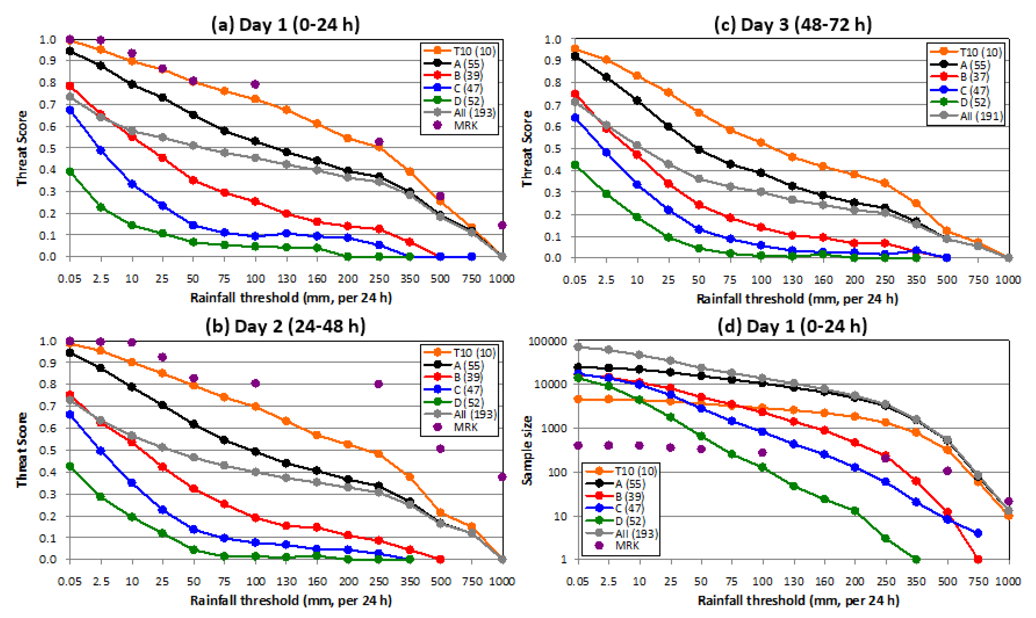
- The overall TS values of day 1 (0–24 h) QPFs for all events were 0.34, 0.28, and 0.18 at 250, 350, and 500 mm, respectively, and the corresponding scores at the three thresholds were 0.31, 0.25, and 0.16 on day 2, and 0.20, 0.15, and 0.08 on day 3. Compared to results from contemporary studies of 5 km models (often from fewer samples for a single season), the above TS values at these high thresholds are higher and represent considerable improvement, especially toward the high thresholds and at ranges beyond day 1. In particular, the day 2 scores are only slightly lower than those of day 1, suggesting a comparable model QPF skill at 24–48 h in relation to 0–24 h.
- (ii)
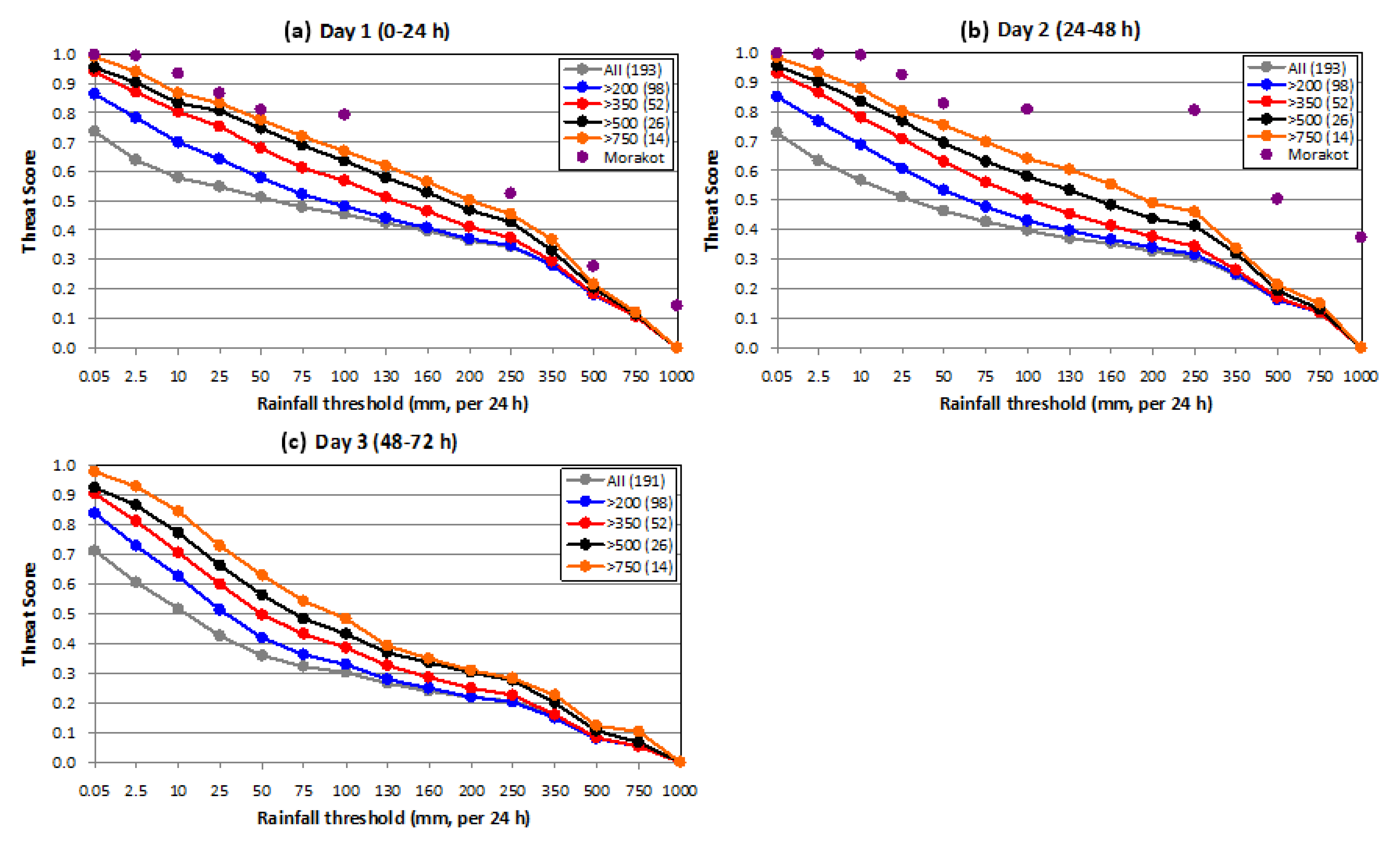
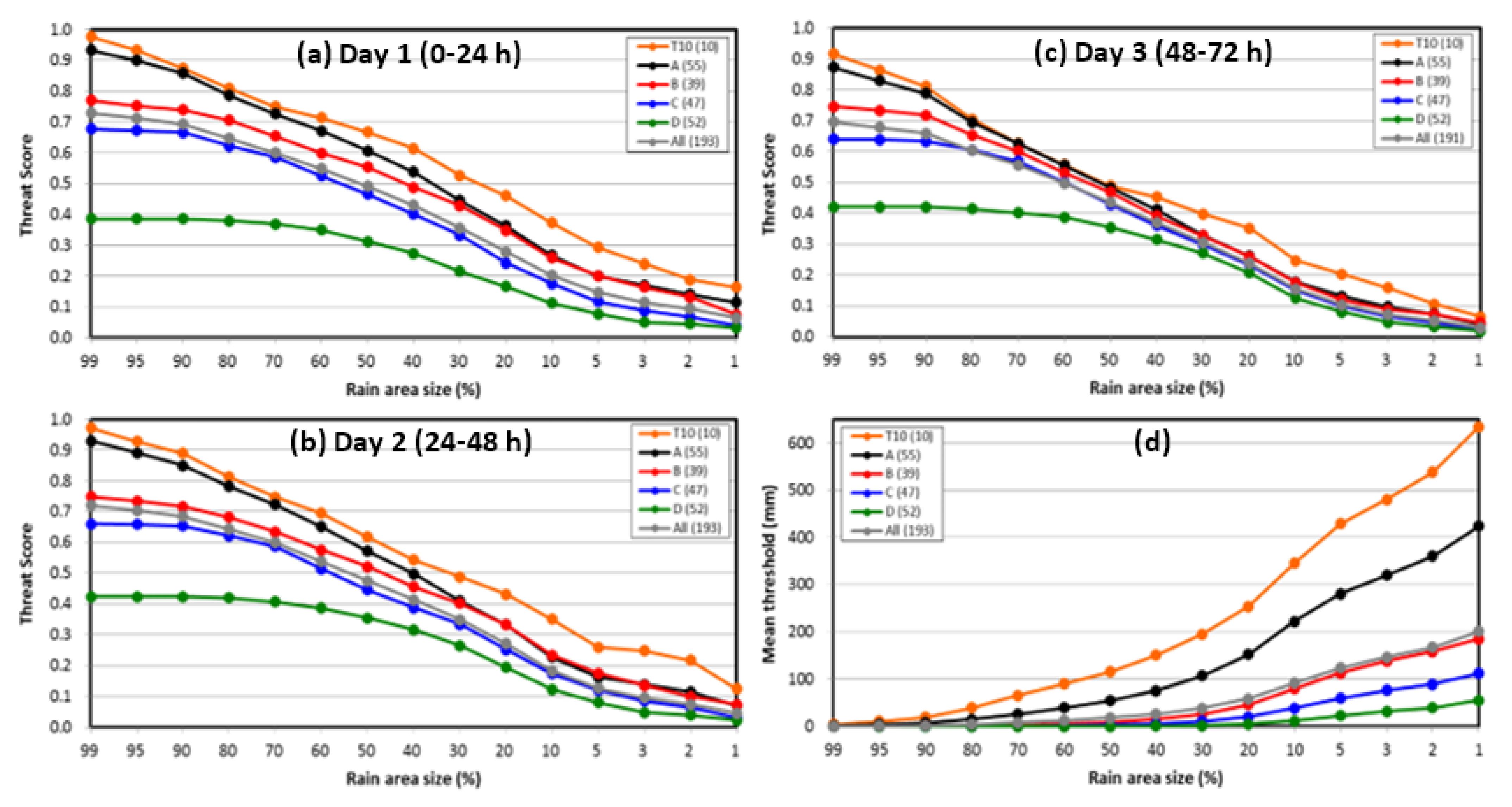
- The dependence found in W15 [31], i.e., higher TSs in larger rainfall events, was also evident in our results here, as expected, and this means a further improved ability to produce QPFs for typhoons with greater rain accumulations in Taiwan. After classification, the TSs for the T10 group (roughly top 5% of events) on day 1, again at 250, 350, and 500 mm, were 0.50, 0.39, and 0.25, respectively, while the corresponding scores were 0.49, 0.38, and 0.21 on day 2, and 0.34, 0.25, and 0.12 on day 3. Using a different and simple classification scheme based on the observed peak rainfall amount, the TSs for the top class (about top 7%, with peak rainfall ≥750 mm) were also similar or slightly lower, indicating that these results are stable and robust. Thus, for the top typhoon rainfall events that have the highest potential for hazards, the 2.5 km CReSS exhibits an improved ability to produce QPFs on the basis of categorical statistics.
- (iii)
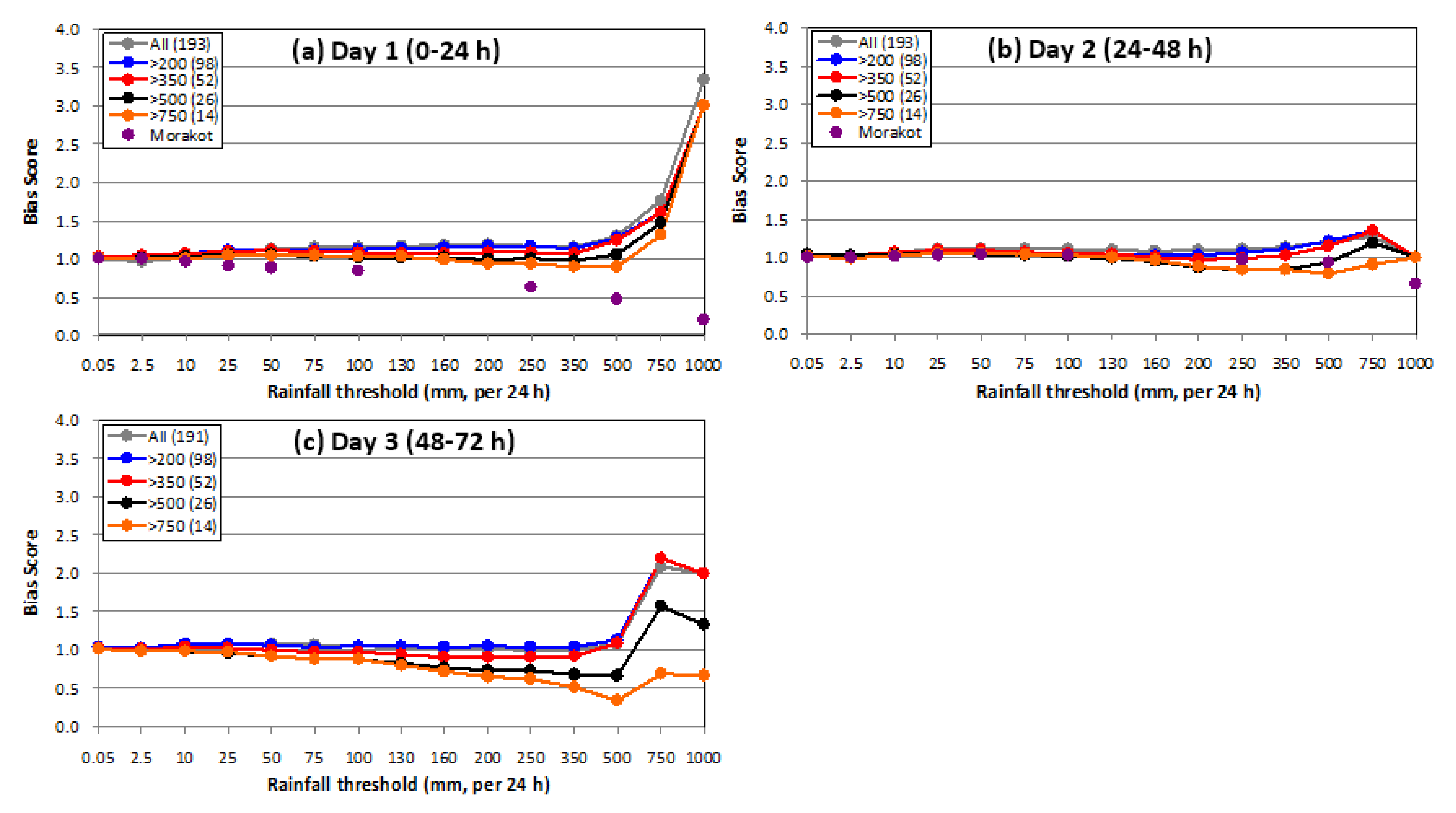
- The classification method based on the observed peak rainfall amount successively filters out subsets of samples with heavier rainfall, and the situations of insufficient points in samples are avoided (as much as possible) even toward the high thresholds. The resultant groups are inclusive and, thus, better suited for categorical statistics, particularly the BS. Overall, the BSs of the 2.5 km CReSS are quite good and especially ideal on day 2, and they show stable results close to unity for all groups across all thresholds with sufficient data points. Thus, the model does not have a tendency to underpredict rainfall toward even the highest threshold, and it is, thus, capable of producing extreme rainfall. For the larger events, nonetheless, there is a slight tendency to under-forecast rainfall toward the higher thresholds.
Author Contributions
Funding
Data Availability Statement
Acknowledgments
Conflicts of Interest
References
- Olson, D.A.; Junker, N.W.; Korty, B. Evaluation of 33 Years of Quantitative Precipitation Forecasting at the NMC. Wea. Forecast. 1995, 10, 498–511. [Google Scholar] [CrossRef] [Green Version]
- Golding, B.W. Quantitative Precipitation Forecasting in the UK. J. Hydrol. 2000, 239, 286–305. [Google Scholar] [CrossRef]
- Mullen, S.L.; Buizza, R. Quantitative Precipitation Forecasts over the United States by the ECMWF Ensemble Prediction System. Mon. Wea. Rev. 2001, 129, 638–663. [Google Scholar] [CrossRef]
- Fritsch, J.M.; Carbone, R.E. Improving quantitative precipitation forecasts in the warm season. A USWRP research and development strategy. Bull. Amer. Meteor. Soc. 2004, 85, 955–965. [Google Scholar] [CrossRef] [Green Version]
- Cuo, L.; Pagano, T.C.; Wang, Q.J. A review of quantitative precipitation forecasts and their use in short-to medium-range streamflow forecasting. J. Hydormeteor. 2011, 12, 713–728. [Google Scholar] [CrossRef]
- Clark, A.J.; Gallus, W.A., Jr.; Chen, T.-C. Comparison of the diurnal precipitation cycle in convection-resolving and non-convection-resolving mesoscale models. Mon. Wea. Rev. 2007, 135, 3456–3473. [Google Scholar] [CrossRef] [Green Version]
- Clark, A.J.; Gallus, W.A., Jr.; Xue, M.; Kong, F. A comparison of precipitation forecast skill between small convection-allowing and large convection-parameterizing ensembles. Wea. Forecast. 2009, 24, 1121–1140. [Google Scholar] [CrossRef] [Green Version]
- DeMaria, M.; Knaff, J.A.; Sampson, C. Evaluation of long-term trends in tropical cyclone intensity forecasts. Meteor. Atmos. Phys. 2007, 97, 19–28. [Google Scholar] [CrossRef]
- Rogers, R.; Aberson, S.; Aksoy, A.; Annane, B.; Black, M.; Cione, J.; Dorst, N.; Dunion, J.; Gamache, J.; Goldenberg, S.; et al. NOAA’s Hurricane Intensity Forecasting Experiment: A Progress Report. Bull. Amer. Meteor. Soc. 2013, 94, 859–882. [Google Scholar] [CrossRef] [Green Version]
- Tallapragada, V.; Kieu, C.; Trahan, S.; Liu, Q.; Wang, W.; Zhang, Z.; Tong, M.; Zhang, B.; Zhu, L.; Strahl, B. Forecasting Tropical Cyclones in the Western North Pacific Basin Using the NCEP Operational HWRF Model: Model Upgrades and Evaluation of Real-Time Performance in 2013. Wea. Forecast. 2016, 31, 877–894. [Google Scholar] [CrossRef]
- Schaefer, J.T. The critical success index as an indicator of warning skill. Wea. Forecast. 1990, 5, 570–575. [Google Scholar] [CrossRef] [Green Version]
- Wilks, D.S. Statistical Methods in the Atmospheric Sciences; Academic Press: Cambridge, MA, USA, 1995; p. 467. [Google Scholar]
- Ebert, E.E.; Damrath, U.; Wergen, W.; Baldwin, M.E. The WGNE assessment of short-term quantitative precipitation forecasts (QPFs) from operational numerical weather prediction models. Bull. Amer. Meteor. Soc. 2003, 84, 481–492. [Google Scholar] [CrossRef]
- Jolliffe, I.T.; Stephenson, D.B. Forecast Verification: A Practitioner’s Guide in Atmospheric Science; Wiley and Sons: Hoboken, NY, USA, 2003; p. 240. [Google Scholar]
- Ebert, E.E.; McBride, J.L. Verification of precipitation in weather systems: Determination of systematic errors. J. Hydrol. 2000, 239, 179–202. [Google Scholar] [CrossRef]
- Davis, C.; Brown, B.; Bullock, R. Object-based verification of precipitation forecasts. Part I: Methodology and application to mesoscale rain areas. Mon. Wea. Rev. 2006, 134, 1772–1784. [Google Scholar] [CrossRef] [Green Version]
- Marzban, C.; Sandgathe, S. Cluster analysis for verification of precipitation fields. Wea. Forecast. 2006, 21, 824–838. [Google Scholar] [CrossRef] [Green Version]
- Wernli, H.; Paulat, M.; Hagen, M.; Frei, C. SAL—A novel quality measure for the verification of quantitative precipitation forecasts. Mon. Wea. Rev. 2008, 136, 4470–4487. [Google Scholar] [CrossRef] [Green Version]
- Wang, C.-C.; Paul, S.; Lee, D.-I. Evaluation of rainfall forecasts by three mesoscale models during the Mei-yu season of 2008 in Taiwan. Part II: Development of an object-oriented method. Atmosphere 2020, 11, 939. [Google Scholar] [CrossRef]
- Wang, C.-C.; Paul, S.; Lee, D.-I. Evaluation of rainfall forecasts by three mesoscale models during the Mei-yu season of 2008 in Taiwan. Part III: Application of an object-oriented verification method. Atmosphere 2020, 11, 705. [Google Scholar] [CrossRef]
- Chen, G.T.J.; Shieh, S.L.; Chen, L.F.; Chen, C.D. On the forecast skill of heavy rainfall in Taiwan. Atmos. Sci. 1991, 19, 177–188. [Google Scholar]
- Hsu, J.C.-S.; Wang, C.-J.; Chen, P.-Y.; Chang, T.-H.; Fong, C.-T. Verification of quantitative precipitation forecasts by the CWB WRF and ECMWF on 0.125 grid. In Proceedings of the 2014 Conference on Weather Analysis and Forecasting, Central Weather Bureau, Taipei, Taiwan, 16–18 September 2014; pp. A2–A24. [Google Scholar]
- Huang, T.-H.; Yeh, S.-H.; Lu, G.-C.; Hong, J.-S. A synthesis and comparison of QPF verifications at the CWB and major NWP guidance. In Proceedings of the 2015 Conference on Weather Analysis and Forecasting, Central Weather Bureau, Taipei, Taiwan, 15–17 September 2015; pp. 7–11. [Google Scholar]
- Tsai, C.-C.; Hsiao, L.-F.; Chen, D.-S.; Bao, C.-W.; Lee, C.-S. Evaluation of the Performance of Hurricane WRF Model over the Western North Pacific in 2013. In Proceedings of the 2014 Conference on Weather Analysis and Forecasting, Central Weather Bureau, Taipei, Taiwan, 16–18 September 2014; pp. A2–A45. [Google Scholar]
- Wang, C.-J.; Huang, L.-J.; Hsiao, L.-F.; Lee, C.-S. Analysis and Discussion on the Results of Taiwan-Area Precipitation Ensemble Experiment (TAPEX) in 2014. In Proceedings of the 2014 Conference on Weather Analysis and Forecasting, Central Weather Bureau, Taipei, Taiwan, 16–18 September 2014; pp. A2–A22. [Google Scholar]
- Skamarock, W.C.; Klemp, J.B.; Dudhia, J.; Gill, D.O.; Barker, D.M.; Wang, W.; Powers, J.G. A Description of the Advanced Research WRF Version 2; NCAR Technical Note: Boulder, CO, USA, 2005; p. 88. [Google Scholar] [CrossRef]
- Biswas, M.K.; Abarca, S.; Bernardet, L.; Ginis, I.; Grell, E.; Iacono, M.; Kalina, E.; Liu, B.; Liu, Q.; Marchok, T.; et al. Hurricane Weather Research and Forecasting (HWRF) Model: 2018 Scientific Documentation. Developmental Testbed Center; Developmental Testbed Center: Boulder, CO, USA, 2018; p. 112. Available online: http://www.dtcenter.org/sites/default/files/community-code/hwrf/docs/scientific_documents/HWRFv4.0a_ScientificDoc.pdf (accessed on 1 October 2021).
- Tsai, C.-C.; Hsiao, L.-F.; Chen, D.-S.; Bao, C.-W.; Lee, C.-S. Evaluation of the performance of hurricane WRF and typhoon WRF models in track and rainfall over the Western North Pacific. In Proceedings of the 2014 Conference on Weather Analysis and Forecasting, Central Weather Bureau, Taipei, Taiwan, 16–18 September 2014; pp. 2–11. [Google Scholar]
- Tsuboki, K.; Sakakibara, A. Large-scale parallel computing of cloud resolving storm simulator. In High Performance Computing; Zima, H.P., Joe, K., Sato, M., Seo, Y., Shimasaki, M., Eds.; Springer: Berlin/Heidelberg, Germany, 2002; pp. 243–259. [Google Scholar]
- Tsuboki, K.; Sakakibara, A. Numerical Prediction of High-Impact Weather Systems—The Textbook for the Seventeenth IHP Training Course in 2007; Hydrospheric Atmospheric Research Center: Nagoya, Japan, 2007; p. 273. [Google Scholar]
- Wang, C.-C. The More Rain, the Better the Model Performs—The Dependency of Quantitative Precipitation Forecast Skill on Rainfall Amount for Typhoons in Taiwan. Mon. Wea. Rev. 2015, 143, 1723–1748. [Google Scholar] [CrossRef]
- Wang, C.-C. Corrigendum. Mon. Wea. Rev. 2016, 144, 3031–3033. [Google Scholar] [CrossRef]
- Wang, C.-C. Paper of Notes: The More Rain from Typhoons, the Better the Models Perform. Bull. Amer. Meteor. Soc. 2016, 97, 16–17. [Google Scholar]
- Liu, A.Q.; Moore, G.W.K.; Tsuboki, K.; Renfrew, I.A. A High-Resolution Simulation of Convective Roll Clouds During a Cold-Air Outbreak. Geophys. Res. Lett. 2004, 31, L03101. [Google Scholar] [CrossRef] [Green Version]
- Wang, C.-C.; Kuo, H.-C.; Chen, Y.-H.; Huang, H.-L.; Chung, C.-H.; Tsuboki, K. Effects of Asymmetric Latent Heating on Typhoon Movement Crossing Taiwan: The Case of Morakot (2009) with Extreme Rainfall. J. Atmos. Sci. 2012, 69, 3172–3196. [Google Scholar] [CrossRef]
- Wang, C.-C.; Kuo, H.-C.; Yeh, T.-C.; Chung, C.-H.; Chen, Y.-H.; Huang, S.-Y.; Wang, Y.-W.; Liu, C.-H. High-Resolution Quantitative Precipitation Forecasts and Simulations by the Cloud-Resolving Storm Simulator (CReSS) for Typhoon Morakot (2009). J. Hydrol. 2013, 506, 26–41. [Google Scholar] [CrossRef]
- Akter, N.; Tsuboki, K. Numerical Simulation of Cyclone Sidr Using a Cloud-Resolving Model: Characteristics and Formation Process of an Outer Rainband. Mon. Wea. Rev. 2012, 140, 789–810. [Google Scholar] [CrossRef]
- Kuo, H.-C.; Tsujino, S.; Huang, C.-C.; Wang, C.-C.; Tsuboki, K. Diagnosis of the Dynamic Efficiency of Latent Heat Release and the Rapid Intensification of Supertyphoon Haiyan (2013). Mon. Wea. Rev. 2019, 147, 1127–1147. [Google Scholar] [CrossRef]
- Wang, C.-C.; Chen, Y.-H.; Li, M.-C.; Kuo, H.-C.; Tsuboki, K. On the Separation of Upper and Low-Level Centres of Tropical Storm Kong-Rey (2013) near Taiwan in Association with Asymmetric Latent Heating. Quart. J. Roy. Meteor. Soc. 2021, 147, 1135–1149. [Google Scholar] [CrossRef]
- Lin, Y.-L.; Farley, R.D.; Orville, H.D. Bulk Parameterization of the Snow Field in a Cloud Model. J. Climate Appl. Meteor. 1983, 22, 1065–1092. [Google Scholar] [CrossRef] [Green Version]
- Cotton, W.R.; Tripoli, G.J.; Rauber, R.M.; Mulvihill, E.A. Numerical Simulation of the Effects of Varying Ice Crystal Nucleation Rates and Aggregation Processes on Orographic Snowfall. J. Clim. Appl. Meteor. 1986, 25, 1658–1680. [Google Scholar] [CrossRef] [Green Version]
- Murakami, M. Numerical Modeling of Dynamical and Microphysical Evolution of an Isolated Convective Cloud—The 19 July 1981 CCOPE Cloud. J. Meteor. Soc. Jpn. 1990, 68, 107–128. [Google Scholar] [CrossRef] [Green Version]
- Ikawa, M.; Saito, K. Description of a nonhydrostatic model developed at the Forecast Research Department of the MRI. MRI Tech. Rep. 1991, 28, 238. [Google Scholar]
- Murakami, M.; Clark, T.L.; Hall, W.D. Numerical Simulations of Convective Snow Clouds over the Sea of Japan: Two-Dimensional Simulation of Mixed Layer Development and Convective Snow Cloud Formation. J. Meteor. Soc. Jpn. 1994, 72, 43–62. [Google Scholar] [CrossRef] [Green Version]
- Deardorff, J.W. Stratocumulus-Capped Mixed Layers Derived from a Three-Dimensional Model. Bound. -Layer Meteorol. 1980, 18, 495–527. [Google Scholar] [CrossRef]
- Kondo, J. Heat balance of the China Sea during the air mass transformation experiment. J. Meteor. Soc. Jpn. 1976, 54, 382–398. [Google Scholar] [CrossRef] [Green Version]
- Louis, J.F.; Tiedtke, M.; Geleyn, J.F. A Short History of the Operational PBL Parameterization at ECMWF. Workshop on Planetary Boundary Layer Parameterization; ECMWF: Reading, UK, 1981; pp. 59–79. [Google Scholar]
- Segami, A.; Kurihara, K.; Nakamura, H.; Ueno, M.; Takano, I.; Tatsumi, Y. 1989: Operational Mesoscale Weather Prediction with Japan Spectral Model. J. Meteor. Soc. Jpn. 1989, 67, 907–924. [Google Scholar] [CrossRef] [Green Version]
- Done, J.; Davis, C.A.; Weisman, M. The Next Generation of NWP: Explicit Forecasts of Convection Using the Weather Research and Forecasting (WRF) Model. Atmos. Res. Lett. 2004, 5, 110–117. [Google Scholar] [CrossRef]
- Liu, C.; Moncrieff, M.W.; Tuttle, J.D.; Carbone, R.E. Explicit and Parameterized Episodes of Warm-Season Precipitation over the Continental United States. Adv. Atmos. Sci. 2006, 23, 91–105. [Google Scholar] [CrossRef]
- Roberts, N.M.; Lean, H.W. Scale-Selective Verification of Rainfall Accumulations from High-Resolution Forecasts of Convective Events. Mon. Wea. Rev. 2008, 136, 78–97. [Google Scholar] [CrossRef]
- Kanamitsu, M. Description of the NMC Global Data Assimilation and Forecast System. Wea. Forecast. 1989, 4, 335–342. [Google Scholar] [CrossRef] [Green Version]
- Kalnay, E.; Kanamitsu, M.; Baker, W.E. Global Numerical Weather Prediction at the National Meteorological Center. Bull. Amer. Meteor. Soc. 1990, 71, 1410–1428. [Google Scholar] [CrossRef]
- Moorthi, S.; Pan, H.L.; Caplan, P. Changes to the 2001 NCEP Operational MRF/AVN Global Analysis/Forecast System. Tech. Proced. Bull. 2001, 484, 14. [Google Scholar]
- Kleist, D.T.; Parrish, D.F.; Derber, J.C.; Treadon, R.; Wu, W.S.; Lord, S. 2009: Introduction of the GSI into the NCEP global data assimilation system. Wea. Forecast. 2009, 24, 1691–1705. [Google Scholar] [CrossRef] [Green Version]
- Hsu, J. ARMTS up and running in Taiwan. Väisälä News 1998, 146, 24–26. [Google Scholar]
- Wang, C.-C. On the calculation and correction of equitable threat score for model quantitative precipitation forecasts for small verification areas: The example of Taiwan. Wea. Forecast. 2014, 29, 788–798. [Google Scholar] [CrossRef]
- Wang, C.-C.; Chuang, P.-Y.; Chang, C.-S.; Tsuboki, K.; Huang, S.-Y.; Leu, G.-C. Evaluation of mei-yu heavy-rainfall quantitative precipitation forecasts in Taiwan by a cloud-resolving model for three seasons of 2012–2014. Nat. Hazards Earth Syst. Sci. 2021. [Google Scholar]
- Feng, J.; Wang, X.G. Impact of assimilating upper-level dropsonde observations collected during the TCI field campaign on the prediction of intensity and structure of Hurricane Patricia (2015). Mon. Wea. Rev. 2019, 147, 3069–3089. [Google Scholar] [CrossRef]
- Feng, J.; Wang, X.G. Impact of increasing horizontal and vertical resolution during the HWRF hybrid EnVar data assimilation on the analysis and prediction of Hurricane Patricia (2015). Mon. Wea. Rev. 2021, 149, 419–441. [Google Scholar] [CrossRef]


| Season | 2010–2011 | 2012 | 2013–2015 |
|---|---|---|---|
| Grid spacing (km) | 2.5 × 2.5 × 0.2−0.663 (0.5) * | ||
| Grid dimension (x, y, z) | 432 × 360 × 40 | 600 × 480 × 40 | |
| Domain size (km) | 1080 × 900 × 20 | 1500 × 1200 × 20 | |
| Forecast interval and range | Every 6 h (initial times at 12:00 a.m., 6:00 a.m., 12:00 p.m., and 6:00 p.m. UTC), 72/78 h | ||
| IC/BCs | NCEP GFS analyses and forecasts (26 levels) | ||
| Grid spacing of IC/BCs | 1.0° × 1.0° | 0.5° × 0.5° | |
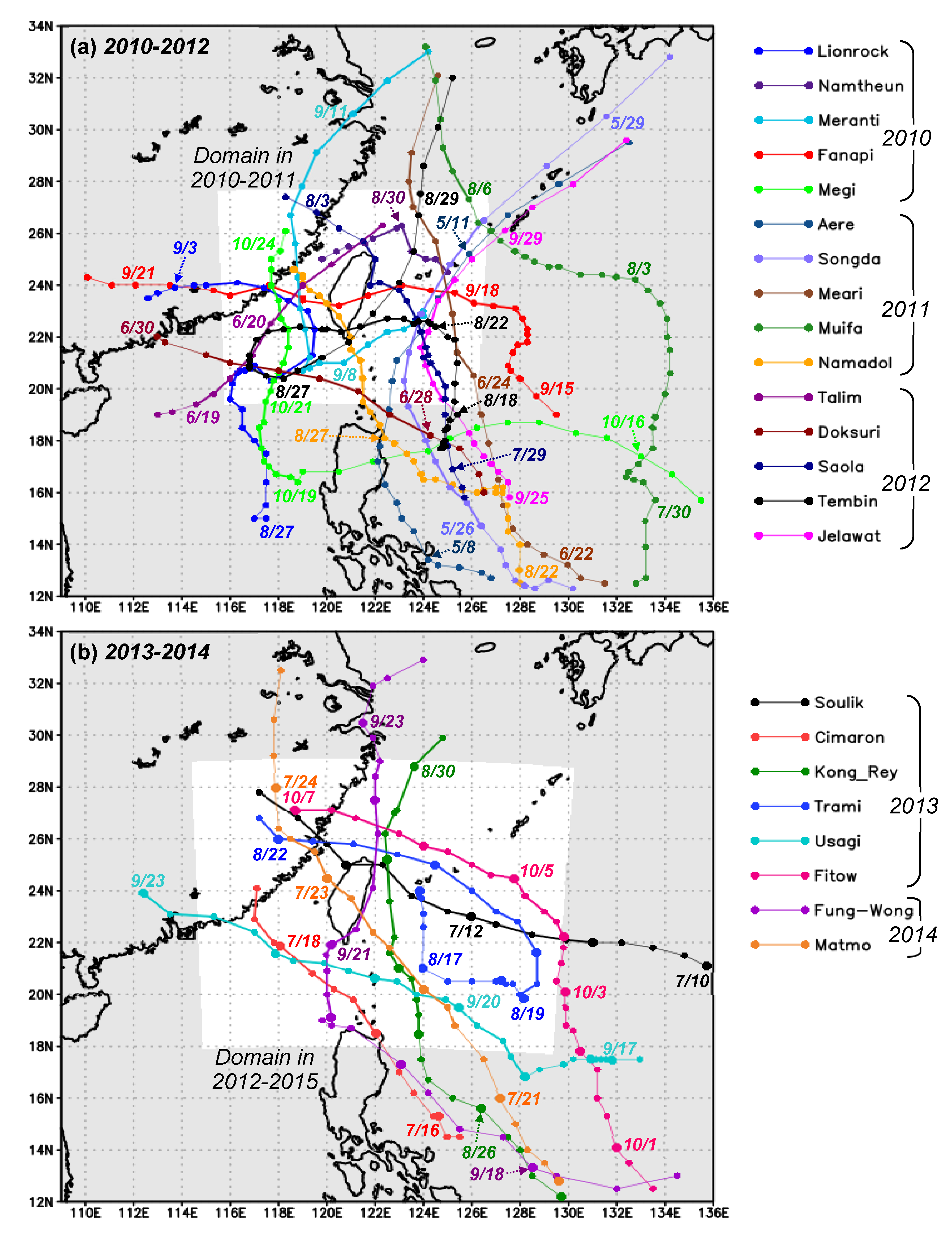
| Name | Data Period | No. of Segments | Classification |
|---|---|---|---|
| Lionrock (2010) | 12:00 a.m. UTC 28 August–12:00 p.m. UTC 3 September | 8 | CC[CBAB]CBACDD |
| Namtheun (2010) | 12:00 a.m. UTC 29–12:00 p.m. UTC 31 August | 4 | CBAB |
| Meranti (2010) | 12:00 a.m. UTC 6–12:00 p.m. UTC 11 September | 10 | DDDDCBBCDC |
| Fanapi (2010) | 12:00 a.m. UTC 16–12:00 p.m. UTC 21 September | 10 | DDDDBATACD |
| Megi (2010) | 12:00 a.m. UTC 19–12:00 p.m. UTC 24 October | 10 | BBBATABCDD |
| Aere (2011) | 12:00 a.m. UTC 9–12:00 a.m. UTC 10 May | 1 | D |
| Songda (2011) | 12:00 a.m. UTC 26–12:00 p.m. UTC 29 May | 6 | CCBCDD |
| Meari (2011) | 12:00 a.m. UTC 24–12:00 p.m. UTC 26 June | 4 | BABC |
| Muifa (2011) | 12:00 a.m. UTC 6–12:00 p.m. UTC 7 August | 2 | DD |
| Nanmadol (2011) | 12:00 a.m. UTC 27 August–12:00 p.m. UTC 1 September | 10 | BAAAAAACCC |
| Talim (2012) | 12:00 a.m. UTC 19–12:00 p.m. UTC 22 June | 6 | BAABCC |
| Doksuri (2012) | 12:00 a.m. UTC 28–12:00 p.m. UTC 30 June | 4 | CCDD |
| Saola (2012) | 12:00 a.m. UTC 30 Jul–12:00 p.m. UTC 3 August | 8 | BAAAATAA |
| Tembin (2012) | 12:00 a.m. UTC 22–12:00 p.m. UTC 28 August | 12 | CCBAABCDDDBB |
| Jelawat (2012) | 12:00 a.m. UTC 27–12:00 p.m. UTC 29 September | 4 | DCCD |
| Soulik (2013) | 12:00 a.m. UTC 11–12:00 p.m. UTC 16 July | 10 | DDATACCCDD |
| Cimaron (2013) | 12:00 a.m. UTC 17–12:00 p.m. UTC 20 July | 6 | CCDDDD |
| Trami (2013) | 12:00 a.m. UTC 19–12:00 p.m. UTC 24 August | 10 | DBAATAABBB |
| Kong-Rey (2013) | 12:00 a.m. UTC 27–12:00 p.m. UTC 31 August | 8 | DDATAAAA |
| Usagi (2013) | 12:00 a.m. UTC 19–12:00 p.m. UTC 24 September | 10 | DDBAAABCDD |
| Fitow (2013) | 12:00 a.m. UTC 4–12:00 p.m. UTC 9 October | 10 | DCCBCDDDDD |
| Matmo (2014) | 12:00 p.m. UTC 21–12:00 p.m. UTC 24 July | 5 | BATAC |
| Fung-Wong (2014) | 12:00 a.m. UTC 20–12:00 p.m. UTC 23 September | 6 | BTABDC |
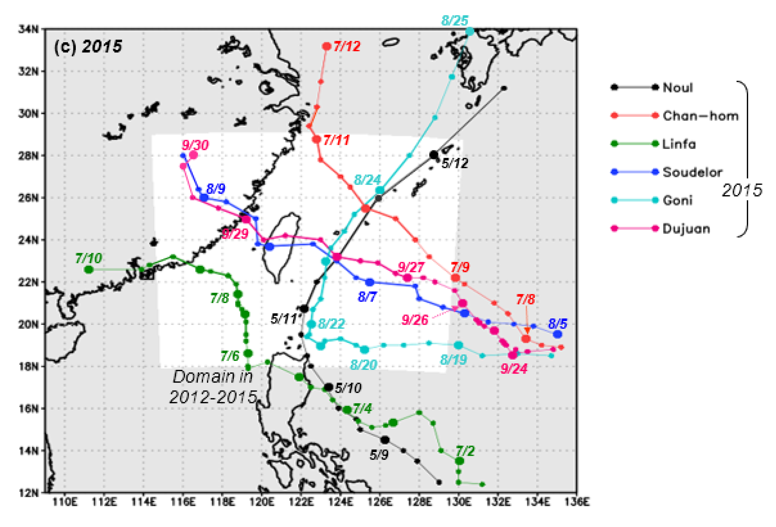
| Noul (2015) | 12:00 a.m. UTC 11–12:00 a.m. UTC 12 May | 1 | C |
| Linfa (2015) | 12:00 p.m. UTC 6–12:00 a.m. UTC 10 July | 6 | CBBCCB |
| Chan-Hom (2015) | 12:00 p.m. UTC 9–12:00 p.m. UTC 11 July | 3 | BBC |
| Souledor (2015) | 12:00 a.m. UTC 6–12:00 p.m. UTC 9 August | 6 | DCATAA |
| Goni (2015) | 12:00 a.m. UTC 20–12:00 p.m. UTC 24 August | 8 | DDCBBBCD |
| Dujuan (2015) | 12:00 a.m. UTC 27–12:00 a.m. UTC 30 September | 5 | CATAD |
| Total | 193 | A: 55, B: 39, C: 47, D: 52 |
Publisher’s Note: MDPI stays neutral with regard to jurisdictional claims in published maps and institutional affiliations. |
© 2021 by the authors. Licensee MDPI, Basel, Switzerland. This article is an open access article distributed under the terms and conditions of the Creative Commons Attribution (CC BY) license (https://creativecommons.org/licenses/by/4.0/).
Share and Cite
Wang, C.-C.; Chang, C.-S.; Wang, Y.-W.; Huang, C.-C.; Wang, S.-C.; Chen, Y.-S.; Tsuboki, K.; Huang, S.-Y.; Chen, S.-H.; Chuang, P.-Y.; et al. Evaluating Quantitative Precipitation Forecasts Using the 2.5 km CReSS Model for Typhoons in Taiwan: An Update through the 2015 Season. Atmosphere 2021, 12, 1501. https://doi.org/10.3390/atmos12111501
Wang C-C, Chang C-S, Wang Y-W, Huang C-C, Wang S-C, Chen Y-S, Tsuboki K, Huang S-Y, Chen S-H, Chuang P-Y, et al. Evaluating Quantitative Precipitation Forecasts Using the 2.5 km CReSS Model for Typhoons in Taiwan: An Update through the 2015 Season. Atmosphere. 2021; 12(11):1501. https://doi.org/10.3390/atmos12111501
Chicago/Turabian StyleWang, Chung-Chieh, Chih-Sheng Chang, Yi-Wen Wang, Chien-Chang Huang, Shih-Chieh Wang, Yi-Shin Chen, Kazuhisa Tsuboki, Shin-Yi Huang, Shin-Hau Chen, Pi-Yu Chuang, and et al. 2021. "Evaluating Quantitative Precipitation Forecasts Using the 2.5 km CReSS Model for Typhoons in Taiwan: An Update through the 2015 Season" Atmosphere 12, no. 11: 1501. https://doi.org/10.3390/atmos12111501
APA StyleWang, C.-C., Chang, C.-S., Wang, Y.-W., Huang, C.-C., Wang, S.-C., Chen, Y.-S., Tsuboki, K., Huang, S.-Y., Chen, S.-H., Chuang, P.-Y., & Chiu, H. (2021). Evaluating Quantitative Precipitation Forecasts Using the 2.5 km CReSS Model for Typhoons in Taiwan: An Update through the 2015 Season. Atmosphere, 12(11), 1501. https://doi.org/10.3390/atmos12111501