Spatial-Temporal Variation of Air PM_2.5 and PM₁₀ within Different Types of Vegetation during Winter in an Urban Riparian Zone of Shanghai

Abstract

Particulate matter (PM) in urban riparian green spaces are undesirable for human participation in outdoor activities, especially PM_2.5 and PM₁₀. The PM deposition, dispersion and modification are influenced by various factors including vegetation, water bodies and meteorological conditions. This study aimed to investigate the impact of vegetation structures and the river’s presence on PM in riparian zones. The spatial-temporal variations of PM_2.5 and PM₁₀ concentrations in three riparian vegetation communities with different structures (open grassland (G), arbor-grass (AG) and arbor-shrub-grass (ASG) woodlands) were monitored under relatively stable environment. The removal percentages (RP) and ratios of PM_2.5 and PM₁₀ were calculated and compared to identify the removal effect of vegetation structures and the river’s presence. It is found that: (1) when the wind was static (hourly wind speed < 0.2 m/s), the RP was ranked as follows: G > AG > ASG. When the wind was mild (0.2 m/s < hourly wind speed < 2 m/s), the RP was ranked as follows: G > ASG > AG. Generally, the G had the best removal effect during the monitoring period; (2) the lowest RP occurred in the middle of the G (–3.4% for PM_2.5, 1.8% for PM₁₀) while the highest RP were found in middle of the AG and ASG, respectively (AG: 2.1% for PM_2.5, 6.7% for PM₁₀; ASG: 2.4% for PM_2.5, 6.3% for PM₁₀). Vegetation cover changed the way of natural deposition and dispersion; (3) compared with static periods, PM removal percentages were significantly reduced under mild wind conditions, and they were positively correlated with wind speed during the mild-wind period. Thus, a piecewise function was inferred between wind speed and PM removal percentage; (4) for all three communities, the 1 m-to-river PM_2.5/PM₁₀ ratio was significantly lower than that at 6 m and 11 m, even lower than that in the ambient atmosphere. The river likely promoted the hygroscopic growth of PM_2.5 and the generation of larger-sized particles by coagulation effect. Based on these findings, open grassland space is preferred alongside rivers and space for outdoor activities is suggested under canopies in the middle of woodlands.

1. Introduction

Particulate matter (PM) exposure is an increasingly severe threat to public health and has been identified as a contributor to cardiovascular and respiratory diseases [1,2,3]. According to epidemiological studies, short-term PM_2.5 exposure is associated with increased all-cause mortality and respiratory diseases mortality [4]. Even relatively low concentrations of air pollutants can lead to high exposure risks [5]. Currently, particulate pollution remains a serious environmental problem in China, especially PM_2.5 pollution. According to the 2019 China Ecological and Environmental Bulletin, a total of 1666 days of heavy pollution (200 < AQI ≤ 300) and 452 days of severe pollution (AQI > 300) in 337 cities were reported in China during 2019. PM_2.5, PM₁₀ and O₃ are primary causes of heavy air pollution, accounting for 78.8%, 19.8% and 2.0% of heavy pollution, respectively. PM exposure is also a threat to social well-being, preventing citizens from participating in outdoor leisure activities, especially during winter when high humidity and little rain leads to heavy air pollution [6]. Inhabitants of megacities such as Shanghai are experiencing enormous health risks caused by PM pollution. Thus, PM removal and mitigation in urban green spaces are priorities for public health.

As the urban population increases, urban rivers have great potential for recreational activities for urbanites [7]. However, urban riparian zones are similarly facing a severe threat of PM exposure, thus causing significant concern. It has already been verified that the association between PM_2.5 and mortality in greener areas was weaker than areas with less greenness of the similar economic conditions [8]. Riparian zones are organic biomes where complex interactions occur between the watercourse, terrestrial environment and riparian vegetation [9]. Accordingly, PM distribution is influenced by the interaction between vegetation and the river in riparian zones. Identifying the influence of vegetation and the river on PM_2.5 and PM₁₀ will help to optimize air quality in urban riparian zones.

It has long been recognized that the vegetation in urban green spaces contributes to the PM removal from the air, primarily through the deposition, dispersion and the modification of PM [10]. The PM capture capacity of a plant is enhanced by the interception of airborne particles and the uptake by leaf surfaces, resulting in high deposition activity [11]. Due to their large leaf surface area [12], the micro morphology [13,14] and epicuticular chemicals [15], plants provide enormous rough surfaces for PM deposition. A tunnel test conducted by Roupsard et al. (2013) proved that the deposition velocity into the artificial grass was 10 to 30 times higher than that onto the smooth urban surfaces such as glass and cement [16]. At a local level, the ability of vegetation to capture PM is more complicated to define. Dispersion, including the processes of sedimentation under gravity, diffusion and turbulent transfer [17], is influenced by multiple factors [18,19,20,21]. The porous structure of trees can alter air flow and increase air turbulence as well as vertical mixing, which contributes to the dispersion and uptake of PM [22,23]. According to Jeanjean et al. (2016), the aerodynamic dispersive effect of trees lead to a 9% reduction in PM_2.5 concentration [24]. Besides, wide and dense vegetation shelterbelt has a significant horizontal reduction effect on total suspended particulate (TSP) and PM₁₀ [25,26]. However, dense trees may impede ventilation and create recirculation zones, keeping PM from dispersion and causing downwind PM accumulation [27,28,29], especially PM_2.5 [26]. Furthermore, small PMs and ultrafine particulates (UFPs) are susceptible to the coagulation effect, which is one type of modification of PM [10]. Yin et al. (2020) found an increase in particle size after resuspension of UFPs from plant leaves, and listed influencing factors such as transpiration, wind and thermal diffusion [30]. Considering this, the role of riparian vegetation in PM removal should be identified and evaluated in the presence of a river.

Previous studies have confirmed that water bodies can efficiently deposit PM. According to the field study of Liu et al. (2016), lakes are better at removing coarse particulate pollution than forests, although forests are better at removing fine PM [31]. Due to strong evaporation and transpiration, water bodies are assumed to exert an effect on PM deposition, probably by increasing relative humidity (RH), decreasing temperature and altering air circulation [32,33,34]. Rivers’ effect on the micro-climate was verified in previous field studies [31,35]. The effect may indirectly influence the PM concentrations and the vegetation removal efficiencies. Compared with lakes in the same area, rivers, as linear elements, have longer aquatic-terrestrial interfaces, and thus, greater interactions with the terrestrial environment, adding to the complexity of the urban ecosystem and the micro climate. This interaction cannot be overlooked when considering PM in the entire heterogeneous urban environment. Few studies have examined the PM concentrations or investigated the removal effect in riparian zones. Therefore, an investigation is required to analyze the individual and interactive effects of riparian vegetation and/or urban rivers on the PM_2.5 and PM₁₀, since this is significant for vegetation design and air pollution reduction.

This study aimed to investigate the impact of vegetation structure and the river’s presence on PM in riparian zones through three types of typical vegetation structure- open grassland (G), arbor-grass (AG) and arbor-shrub-grass (ASG) woodlands. The PM_2.5 and PM₁₀ concentrations were measured by continuous monitoring during a limited period to characterize their spatial differences and temporal variation under a relatively stable macro-environment. Three sampling positions within each typical vegetation community were established to verify the effect of the river. The removal efficiencies and proportions of PM_2.5 and PM₁₀ were calculated and compared under different wind conditions to analyze the effects of vegetation structure and the river’s presence. Moreover, the interaction between the distance to the river and vegetation structures was analyzed to obtain a comprehensive understanding of the intricate processes, including deposition, dispersion and modification. These results provide detailed information for practical vegetation design in riparian zones and expand the current research on how vegetation removes PM in more complicated urban circumstances.

2. Materials and Methods

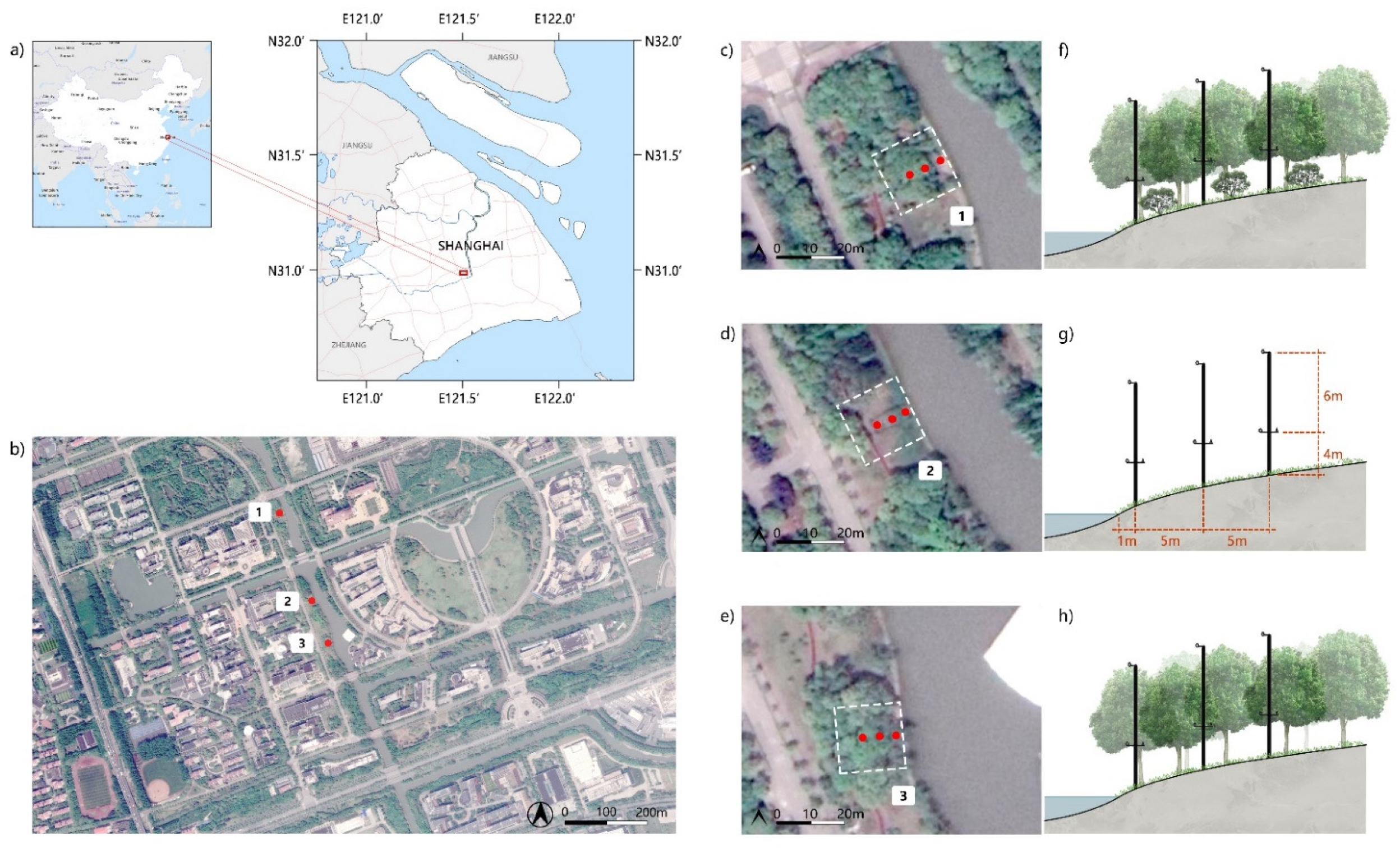
2.1. Study Sites

The study sites (Figure 1) were located beside the Danshui River on the campus of the Shanghai Jiao Tong University, Minhang District, Shanghai, China (31°01′ N, 121°26′ E). Shanghai, located at the estuary of the Yangtze River, is on the Yangtze River delta plain, which is host to a wide range of rivers. It has a humid subtropical climate. Winters are chilly and damp and accompanied by hazy and foggy weather, with an average minimum temperature of 2.1 °C and an average maximum temperature of 11.1 °C (1981–2010). The monthly average RH ranges from 71% to 74% (1981–2010) (China Meteorological Administration). According to the Shanghai Water Authority (2019), there is 29,862 km of rivers and streams in Shanghai. Hundreds of rivers and canals are interconnected, forming a wide water networks. Among them, small-sized rivers with a width under 30 m account for 63.0% of the total area of Shanghai rivers. The Danshui River of 15–20 m’ width was chosen for this study as a representative of small rivers.

Three sample sites in a strip of greenbelt between the Danshui River and a campus road were selected (Figure 1a–c). The green space is 30–40 m wide, containing a pedestrian walking path. In addition, the seven-meter-wide campus road to the west is more than 20 m from these three plots (

Table 1. Sample sites, distance from the road, greenbelt structure and arrangement of plants.

Sample Site	Distance from the Road (m)	Structure Type	Leaf Area Index (LAI)	Porosity (%)	Dominant Species (Height: m)
1	20	Arbor-Shrub-Grass	1.86	11.20	Cinnamomum camphora (9.6), Ginkgo biloba (9.8); Osmanthus fragrans, Camellia japonica (2.5)
2	21	Grass	/	/	Zoysia japonica, Trifolium repens;
2	20	Arbor-Grass	1.24	26.80	Cinnamomum camphora (9.8); Erigeron canadensis, Trifolium repens, Oxalis corymbosa (0.1)

). According to previous studies, the impact range of traffic pollution on the PM_2.5 concentration in roadside vegetation is about 17 m [36] and thus, the impact of the campus road on the particles in the sampling sites is ignored here. As a result, all sample sites were considered to be exposed only to the ambient atmosphere.

Three typical plant communities were selected: open grassland (G), arbor-grass (AG) and arbor-shrub-grass (ASG) woodlands. Therefore, three plots (20 m × 20 m) along the Danshui River were established as the monitoring sites (Table 1). The entire open grassland (G) site was about 30 m long along the river and adjacent to forests on both sides (Figure 1d). The dominant species are Zoysia japonica and Trifolium repens. It was under regular maintenance to ensure that all the herbaceous plants were shorter than 0.3 m. The arbor-grass (AG) woodland was Cinnamomum camphora pure forest, about 30 m wide and 40 m long along the river (Figure 1e). The arbor-shrub-grass (ASG) woodland (35 m wide and 40 m long) was a more closed and complex forest dominated by Cinnamomum camphora and Camellia japonica. Both the AG and the ASG were artificially planted and aged more than 10 years. To quantify and characterize the structure and growth status of riparian vegetation, the leaf area index (LAI) and shelterbelt porosity were measured.

2.2. Field Data Collection and Selection

The PM_2.5 and PM₁₀ concentrations and wind speed were measured at fixed positions along the transects from the edge of the Danshui River (Figure 1d–f). Previous studies have indicated that the impact range of a 15-meter-wide river on the riparian vegetation microclimate is evident up to 18 m, but primarily within 10 m [37] (Zhang and Li, 2007). Thus, three fixed measurement locations were established in stepped proximity from the river edge: 1 m, 6 m and 11 m. Nine locations in total were established to position the instruments. All the sensors were installed 4 m above the ground (Figure 1g,h). A height of 4 m, right under the canopies of the arbor trees, was considered to be appropriate to study the removal effect of the trees. According to Xing and Brimblecombe (2018) [36], receptors at a height of 4 m and a distance of 20 m from the campus road were nearly free of the influence of traffic pollution during long-term measurements. Additionally, the background atmospheric PM concentrations were measured at an elevation of 10 m above the ground, right above the canopies.

Data collection campaign was conducted continuously in December of 2019. Data from the locations were measured and logged at 10 min intervals in real-time and transmitted through a wireless network. Auto-designed measuring stations were installed at all nine locations. Eighteen laser particle probe modules (JXM-PM, V1.0, Weihai JXCT Electronics Co., Ltd., Weihai, China) were used to measure PM_2.5 and PM₁₀ concentrations within the vegetation and from the atmosphere. The detectors had a measuring range of 1 to 999 μg/m³, a resolution of 1 μg/m³, and an error of <±10%. The rated working environment had a temperature range of −30 to 70 °C and a relative humidity range of 0 to 95%. Furthermore, a range of measurements was obtained to characterize the microclimate at each site. Nine wireless temperature and humidity sensors (Weihai JXCT Electronics Co., Ltd., Weihai, China) were used to measure relative humidity (RH) and temperature. The measuring range for RH was from 0 to 100%, with a resolution of 0.1%. The measuring range for temperature was from −40 to 80 °C with a resolution of 0.1 °C. Nine Model 485 wind speed sensors (JXBS-3001-FS, Ver1.0, Weihai JXCT Electronics Co., Ltd., Weihai, China) were used to measure wind speed. The sensors had a measuring range of 0 to 30 m/s, with a resolution of 0.1 m/s and an error of ±1 m/s. All of the instruments were calibrated before leaving the factory and then delivered and installed in the same batch. During the whole monitoring period, the sensors worked under the rated working environment.

This study aimed to investigate the impact of vegetation structure and the river’s presence on PM_2.5 and PM₁₀. Therefore, the influence of climate variables was eliminated as much as possible. The macro-environment conditions needed to remain relatively stable, and the rainfall and wind speed [18,38,39] needed to be controlled. Rainless days with low wind force (1–2 on the Beaufort scale) within a limited time span were the ideal conditions for monitoring. Under these conditions, the minor wind force lowered the influence of wind direction, which could be ignored in the discussion; and it can be assumed that the absorbed and deposited PM would not return to the air, so that the aerodynamic processes were simplified. Thus, the effect of vegetation structure and the river’s presence was presented in the distributions, variations and the proportions of PM_2.5 and PM₁₀. Moreover, the analysis of PM distributions and variations was performed based on different wind speed conditions. Therefore, to better ensure the stability of the weather conditions and to obtain a certain amount of sample data, 48-h (3 and 4 December 2019) continuous monitoring was selected for detailed analysis; these dates were sunny/cloudy with low wind force (1–2).

2.3. Data Analysis

Six sampling data points were averaged to estimate the level of one hour. Some of the AG woodland data were lost due to unstable signal transmission. To obtain a more complete representation of the spatial-temporal distribution of the PM data, the data points were replenished using linear interpolation; this missing data accounted for 10.4% of the entire dataset.

The same process was applied to calculate the background PM concentrations. Because the background data at the 6 m distance from the river in the AG woodland were abnormal due to sensor failure, only the data from the G and the ASG were taken into the calculations of the background concentrations. The results of the ANOVA indicated that the measured background PM concentrations did not significantly differ as a function of vegetation types (p > 0.1). Thus, the assumption that the sampling sites were primarily exposed to an ambient atmosphere was verified to some extent. Therefore, the PM concentration values from the G and the ASG at the same proximity from the river were averaged to represent the background concentration. In the subsequent calculations of PM removal efficiencies, all three sampling sites shared the same background PM concentrations.

Based on the PM_2.5 and PM₁₀ concentrations at a height of 4 m and the background concentrations measured at a height of 10 m, the PM removal percentage (RP) was calculated to indicate the removal efficiency under the confounding effects of vegetation type and the river:

$$\mathrm{Removal} \mathrm{percentage} \left(\mathrm{RP}\right)=\frac{C_{background}-C}{C_{background}}\times 100\%$$

(1)

where C_background (μg/m³) is the hourly PM concentration in ambient atmosphere estimated by the measurement at an elevation of 10 m, right above the tree canopies; C (μg/m³) is the hourly PM concentration measured within the vegetation communities at an elevation of 4 m.

The RP is an estimation of the removal efficiency of the vegetation and the river. The common background concentrations made it possible to compare the removal efficiencies of three vegetation types and stepped distances from the river. This measurement eliminated the effect of background concentrations, meaning the influence of vegetation structure and the distance from the river were better able to be defined.

Additionally, the following statistical methods were used to characterize the patterns in the PM concentrations and analyze the influence of the variables. All data were processed using Excel 2016 and Origin 2020b (Learning Edition).

2.3.1. Analysis of Variance (ANOVA)

The data were grouped into vegetation types, and intra-site comparisons were performed to test the significance of the spatial differences within each vegetation community. Two-way ANOVA was used to assess the effect of vegetation type and proximity from the river, as well as the interaction between the two. In this way, the PM concentrations and removal efficiencies of all nine locations could be compared at an average level. The differences of PM_2.5 and PM₁₀ removal efficiencies as a function of wind conditions were also tested using ANOVA. Additionally, ANOVA was used to test the significance of the spatial differences in ambient PM concentrations and meteorological parameters to reveal the effect of vegetation type and the river on the meteorological parameters.

2.3.2. Hierarchical Cluster Analysis

To characterize the spatial distribution of PM on 3 and 4 December 2019, these two days were segmented into hourly groups. Hence, 48 groups of data were obtained for each site, obtaining 144 groups of data in total. Every group contained six data points (three for PM_2.5 and three for PM₁₀, respectively) reflecting the PM concentrations in the stepped proximities from the river, which, as a whole, represented the spatial distributions of that hour.

A hierarchical cluster analysis was used to recognize possible patterns of spatial distribution among 144 groups of data. Based on the analysis, all data objects were grouped into five clusters. Thus, objects in the same cluster were more similar to each other than to those in other clusters.

2.3.3. Pearson Correlations

Correlations were conducted to test the significance of the relationships between the variables that were intended to be analyzed. Pearson correlations were used to examine relationships between hourly background PM_2.5 and PM₁₀ concentrations, and the hourly levels of the PM_2.5 and PM₁₀ recorded within three vegetation communities. Pearson correlations were also used to test the association between PM removal percentages and meteorological parameters: wind speed, temperature and relative humidity. Additionally, the relationship between the spatial distributions in the removal percentages at stepped proximities from the river and the ambient average wind speed were examined by Pearson correlation to analyze the effect of wind on the spatial distribution. The variance in PM concentrations and removal percentages at three locations along each transect within the vegetation was calculated to identify the evenness of the PM distributions. Wind speed measured in the open grassland (G) at 4 m high were averaged to measure the ambient wind speed.

3. Results and Discussion

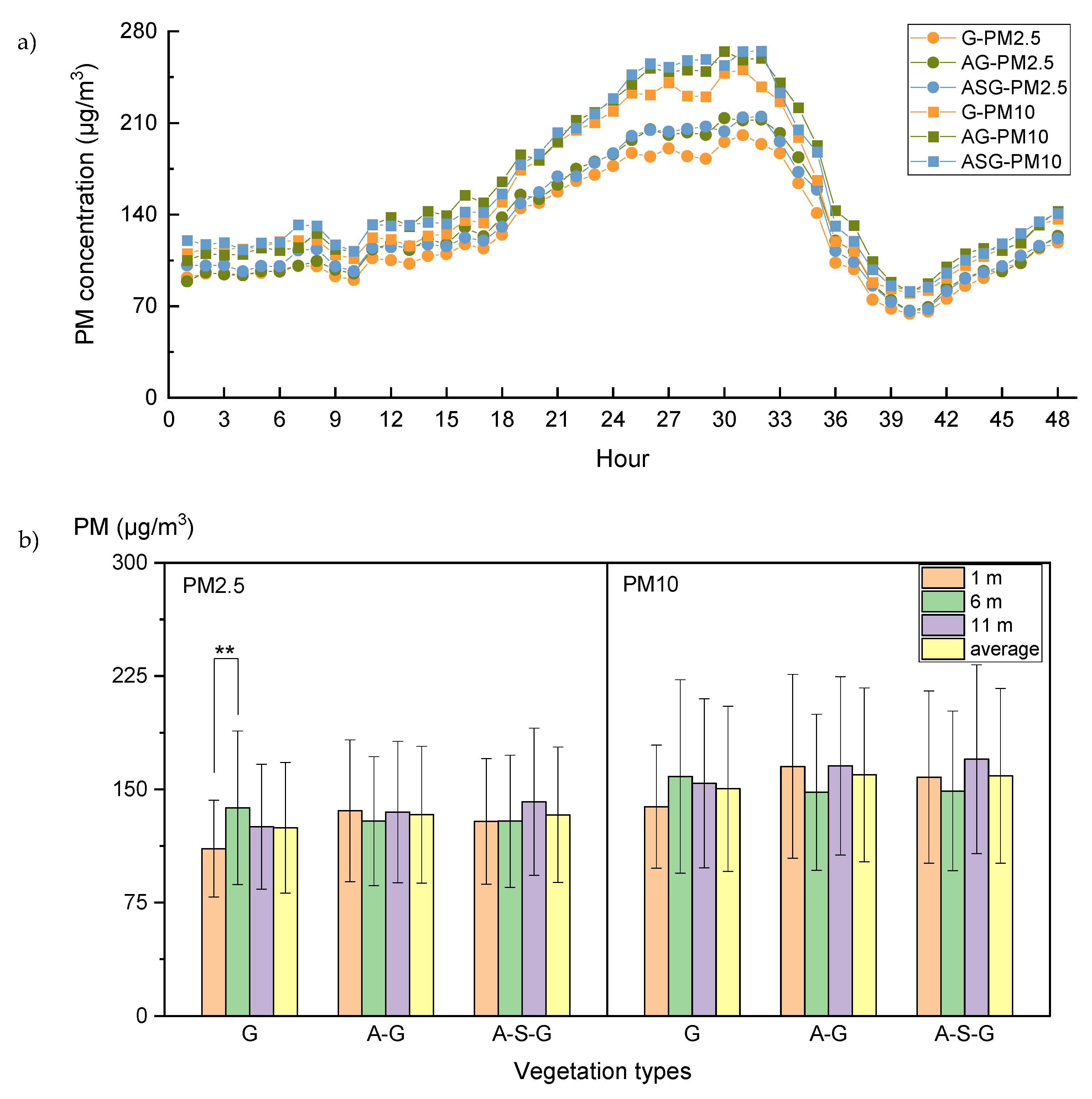
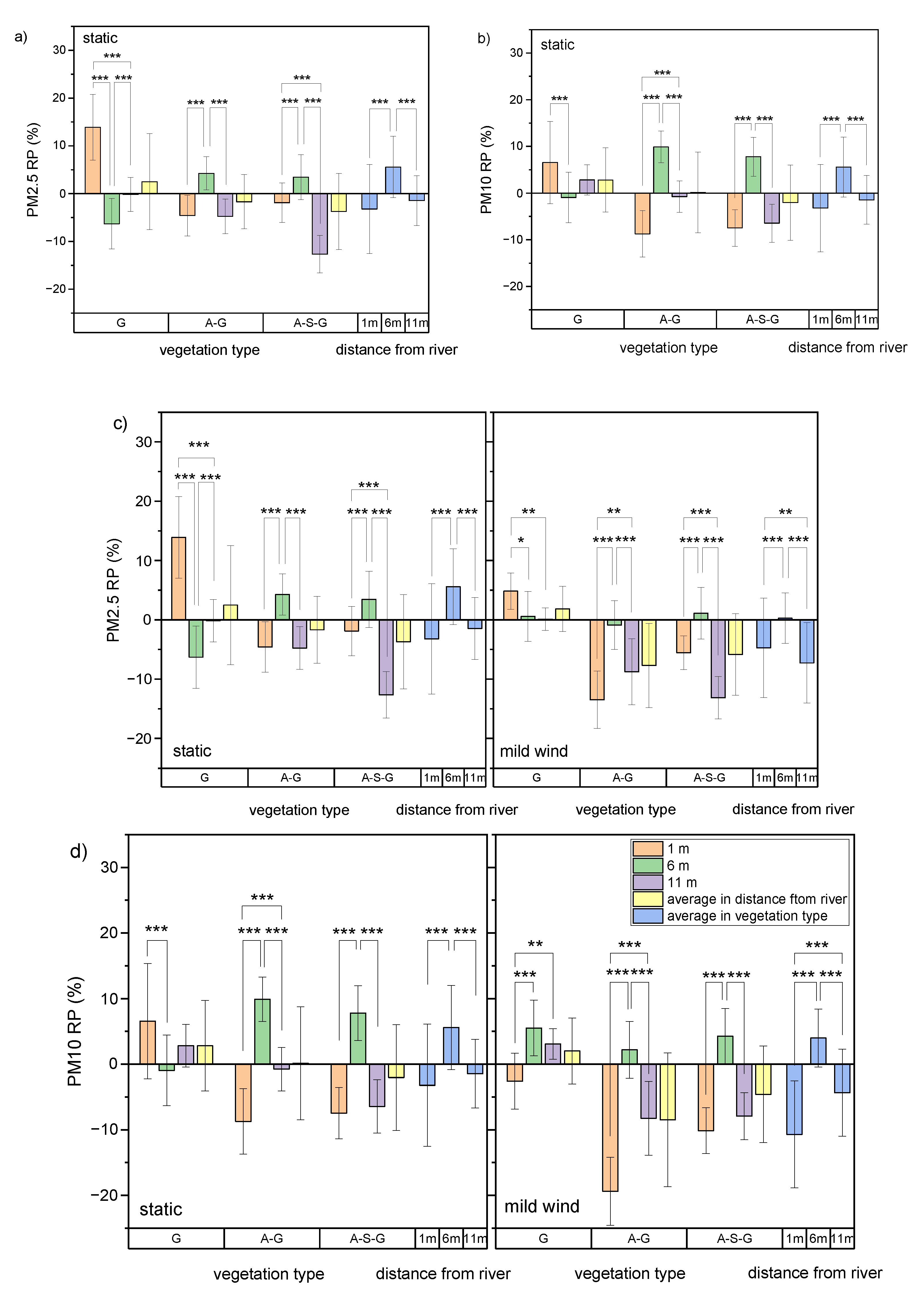
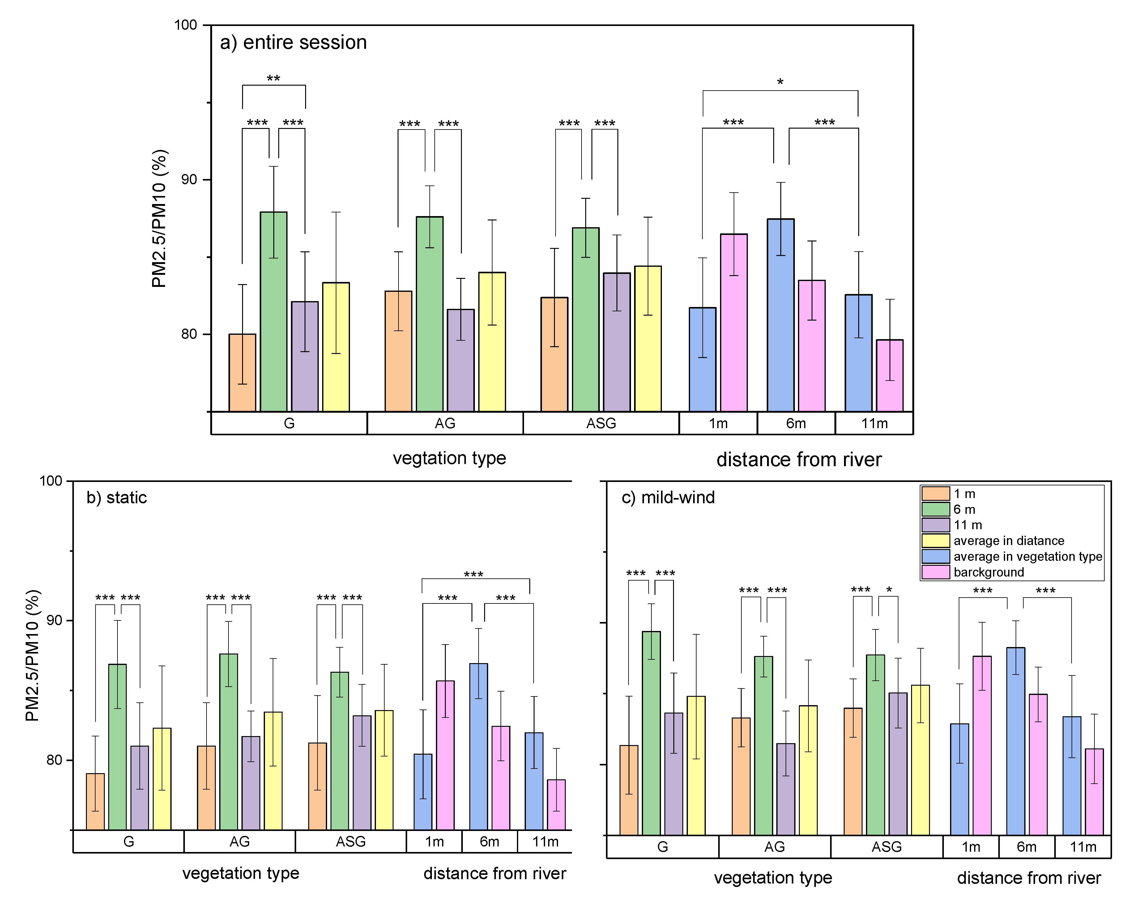
3.1. Spatial-Temporal Variation in the PM Concentrations and Removal Efficiencies

As shown in Figure 2a, the variation of PM_2.5 and PM₁₀ concentrations of three vegetation types in 48 h exhibited the same trend. The highest concentration value occurred from 9:00 p.m. on 3 December to 10:00 a.m. on 4 December, and the average concentrations of all vegetation types were higher than 150 μg/m³. The lowest concentration value occurred from 2:00 p.m. to 6:00 p.m. on 4 December, and the averaged concentrations of all vegetation types were below 90 μg/m³. The 24-h average PM_2.5 and PM₁₀ concentrations during the observation periods exceeded China’s ambient air quality standards (GB 3095—2012). In addition, PM_2.5 comprised more than half of the PM₁₀ mass. Therefore, a reduction strategy was required to lower the high PM concentration.

The average PM_2.5 and PM₁₀ concentrations in the G were slightly lower than those in the AG and the ASG in general, but these differences were not statistically significant (p > 0.05) (Figure 2b). The average PM_2.5 concentration in the G was 124.5 ± 41.1 μg/m³, lower than 132.9 ± 45.4 μg/m³ in the AG and 133.1 ± 44.6 μg/m³ in the ASG. The same pattern can be observed for PM₁₀. The average PM₁₀ concentration in the G was 150.3 ± 53.3 μg/m³, while in the AG it was 159.2 ± 57.2 μg/m³, and in the ASG it was 159.0 ± 57.4 μg/m³. It was primarily due to high dispersion in the open grassland. However, no statistically significant difference was found. It was probably because the dataset included periods with both high concentrations and low concentrations, the standard deviation values for the PM concentrations were relatively high, and the differences as a function of vegetation types were neutralized. For the same reason, the spatial difference was not significant according to the ANOVA (Figure 2b). However, it can be found that the average PM_2.5 and PM₁₀ concentrations at 1 m from the river in the G were the lowest along the transect. The concentration was 110.7 ± 32.0 μg/m³ for PM_2.5 and 138.5 ± 40.8 μg/m³ for PM₁₀.

The temporal-spatial distribution patterns in all vegetation communities are shown in Figure 3a. Hierarchical cluster analysis classified the 48 h into five clusters based on the values and distributions of the PM_2.5 and PM₁₀ concentrations. The results indicated that the open grassland (G) had a different PM spatial distribution from the AG and the ASG woodlands. The most typical differences in the three vegetation types appeared when the peak concentrations were reached. Cluster 4 occurred only in the G form the night of the 3rd to the morning of the 4th: higher concentrations in the middle and lower concentrations at the periphery; cluster 5 mainly occurred in the AG and the ASG during the same periods: lower concentration in the middle and higher at the periphery. At other times, the differences as a function of vegetation types were not statistically significant, even at the dawn of 3 December and the night of 4 December, which were under similar meteorological conditions as the peak period. Therefore, the difference between different vegetation types was probably attributed to the high PM concentration values, instead of specific meteorological conditions.

The spatial distribution of the PM removal efficiencies within the vegetation communities differed distinctly among the three vegetation types (Figure 4b), consistent with the distribution of the PM concentrations (Figure 3a). Specifically, there was a distinct removal effect at the 1 m distance from the river in the G, which is consistent with the previous literature [31]. However, at the 6 m distance from the river, which was in the middle of the open grassland, the removal effect was negative, causing PM_2.5 and PM₁₀ to accumulate. The opposite pattern was observed for the AG and the ASG. Additionally, the spatial difference in the PM removal efficiency was not limited to the peak period, revealing the patterns in a general sense.

The results above indicate that open grassland (G) was not only a control site, but also an exact contrast displaying significantly different patterns. The lower average PM concentrations in the G indicate the natural deposition and high dispersion of PM_2.5 and PM₁₀. However, the higher concentration value in the middle of the community suggests that the deposition effect causes PM accumulation instead of removal. This was probably due to lack of leaf surfaces compared to the arbor-grass (AG) and arbor-shrub-grass (ASG) woodlands. Detailed discussion will be made in the section regarding influencing factors.

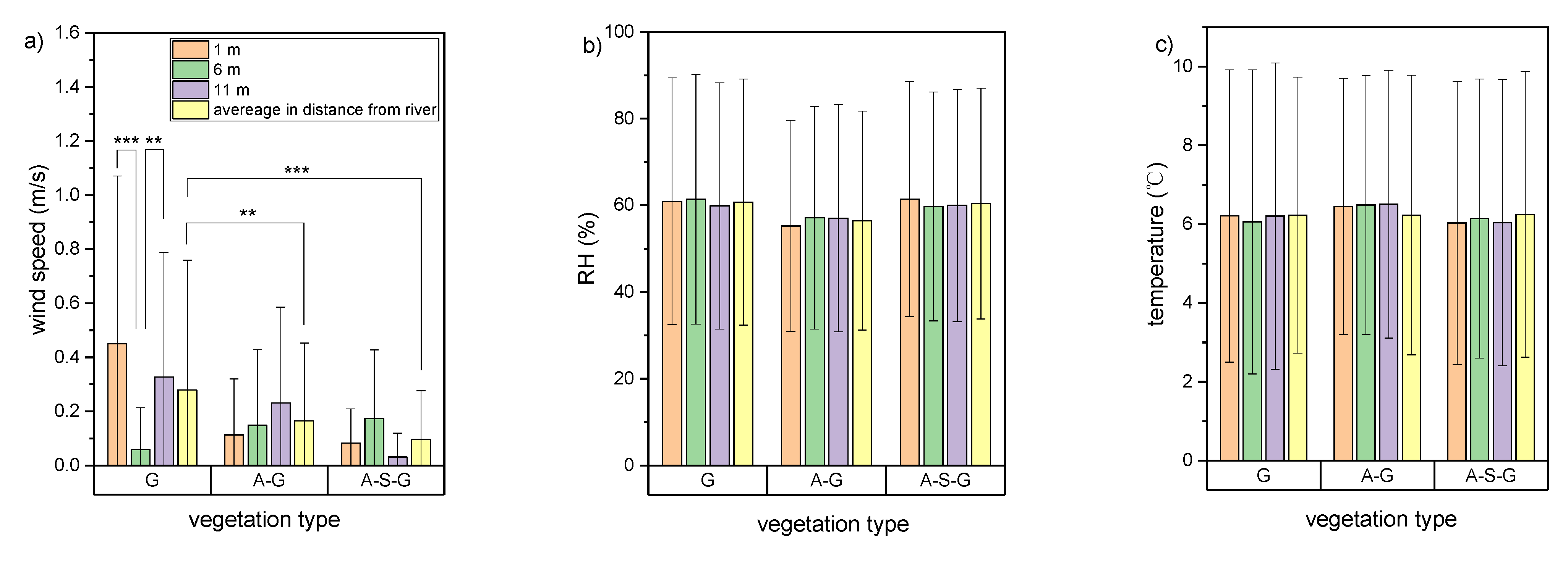
3.2. Spatial Differences in Meteorological Parameters

The results of the ANOVA revealed statistically significant differences in the wind speed at different distances from the river in different vegetation communities (Figure 5a–c). However, the spatial differences in air temperature and relative humidity were not statistically significant, and the influence of these two factors on the distribution of PM in the community can be excluded.

The difference of wind speed as a function of vegetation types and distance from the river explains the spatial distribution of PM concentrations and RP to some extent. The wind speed was the lowest at 6 m from the river along the transect in the G (Figure 5a), causing the lowest RP in the middle the open grassland (Figure 6a,b). The significantly higher wind speed in the G resulted in higher RP than those in the AG and ASG. However, the spatial differences of wind speed in the AG and ASG were not statistically significant. Thus, the spatial differences of PM RP in the AG and ASG will be discussed from other perspectives later.

3.3. Analysis of the Influential Variables

3.3.1. Ambient PM Concentration

The Pearson correlation results (

Table 2. Correlation analysis between the observed PM_2.5 and PM₁₀ concentrations and the background concentrations.

Plant Community Structure		Grass	Arbor-Grass	Arbor-Shrub-Grass
PM2.5	Pearson Corr.	0.95185	0.97887	0.97351
	p-value	8.60 × 0−75	8.74 × 10−100	6.85 × 10−93
PM10	Pearson Corr.	0.97563	0.96024	0.97513
	p-value	1.97 × 10−95	1.44 × 10−80	8.18 × 10−95

) revealed significant positive correlations between the PM concentrations measured within the vegetation and the background PM concentrations during the observing period, inferring that the ambient PM concentration was a key factor influencing the PM concentrations within the vegetation.

3.3.2. Effect of Wind Speed

Wind force ranged from 1–2 on the Beaufort scale during the observation period. The instant wind speed was less than 4.5 m/s, and the hourly average wind speed was less than 2.0 m/s. To better analyze the effect of wind speed, the entire monitoring session was separated into static periods and mild-wind periods based on the hourly average wind speed. Mild wind periods were during the daytime, with hourly wind speeds of 0.2–2 m/s, including 8:00 a.m.–5:59 p.m. on 3 December and 9:00 a.m–6:59 p.m. on 4 December. Static periods occurred at night, with hourly wind speeds under 0.2 m/s, including 0:00–7:59 on the 3rd, 18:00 on the 3rd–8:59 on the 4th, and 19:00–23:59 on the 4th. The statistical analysis of the different wind conditions and the entire observation period is shown in Figure 6 and

Table 3. The average PM removal percentage (RP, unit: %) and wind speed (WS, unit: m/s) statistics for the three types of vegetation.

Plant Community Structure		G	AG	ASG	Average	Significance of the Difference in Vegetation Types
static	PM2.5 RP (%)	2.5 ± 10.0	−1.7 ± 5.7	−3.7 ± 8.0	−0.9 ± 8.5	1
	PM10 RP (%)	2.8 ± 6.9	0.1 ± 8.6	−2.0 ± 8.1	0.3 ± 8.1	1
mild wind	PM2.5 RP (%)	1.8 ± 3.8	−7.7 ± 7.1	−5.9 ± 6.9	−3.9 ± 7.4	1
	PM10 RP (%)	2.0 ± 5.0	−8.5 ± 10.2	−4.6 ± 7.4	−3.7 ± 8.9	1
improvement by wind *	PM2.5 RP (%)	−0.7 ± 10.7	−6.0 ± 9.1	−2.2 ± 10.6	−3.0 ± 11.3
	PM10 RP (%)	−0.8 ± 8.5	−8.6 ± 13.3	−2.6 ± 11.0	−4.0 ± 12.0
wind speed under mild-wind condition (m/s)		0.67 ± 0.55	0.39 ± 0.33	0.23 ± 0.22	0.18 ± 0.35	1
significance of difference in wind condition		0	1	0	1

* improvement by wind = RP_{mild wind}-RP_static; G: open grassland; AG: arbor-grass woodland; ASG: arbor-shrub-grass woodland.

.

The average PM_2.5 and PM₁₀ removal percentages under mild wind conditions were significantly lower than those during the static periods (p < 0.001) (Table 3). Specifically, mild wind caused a significant decrease in the PM removal percentages in the AG. This result suggests a negative effect of mild wind on the PM removal efficiency in the AG, which is consistent with the results of several previous studies. Lee et al. (2018) reported that PM_2.5 and ultrafine particles (UPFs) reductions dropped with increasing wind speed when the wind speed was under 2 m/s [19]. Qiu et al. (2018) also found an increase in the PM_2.5 and PM₁₀ concentrations with wind velocity during sunny and breezy weather [40]. Gravitational deposition is the primary pathway of PM removal under static conditions. However, mild wind probably increases the complexity of the aerodynamic processes. When the wind speed is mild (approximately 1 m/s), laminar flow occurs with little turbulence dispersion and mixing (Jeanjean et al., 2016). Therefore, it can be inferred that mild wind likely causes lower removal efficiency compared to static conditions. Further discussion about the differences between the three vegetation types will be presented in the next section.

Despite the negative effect of mild wind, the Pearson correlation results during the mild-wind periods revealed a positive correlation between wind speed and PM_2.5 removal percentages (p < 0.001). The Pearson correlation results from the data points of the G and the ASG also revealed positive correlations between wind speeds and PM_2.5 removal percentages (p < 0.05 for the G, p < 0.001 for the ASG). However, the results showed that the relationship between wind speeds and PM₁₀ removal percentages was controversial. Data points from the ASG indicated a positive correlation, but data points from the G suggested the opposite. Overall, these results indicated that higher wind has a better removal effect on PM_2.5 and the influence of mild wind on PM₁₀ is more complicated. What is noticeable is that the positive correlation between PM_2.5 removal percentage and wind speed under mild-wind conditions cannot be integrated with the significantly higher PM_2.5 removal percentage under static conditions. This contradiction demonstrates that PM removal percentage is a piecewise function of wind speed. Therefore, more data from controlled experiments under other wind conditions are required to further investigate how the removal percentage varies with increasing wind speed.

The scatter graphs shown in Figure 7a,b indicated that the influence of wind speed tended to become dominant as it increased. When the wind speed was under 1 m/s, PM_2.5 and PM₁₀ removal percentages ranged from −20% to 20%. The high dispersion degree indicated the impact of other variables, such as the distance from the river and the vegetation structure. As the wind speed increased, the PM_2.5 and PM₁₀ removal percentages fell into a more limited range and were likely to increase as the wind speed increased further. However, for higher wind speeds, more investigations are required to verify this tentative conclusion. Additionally, the PM removal percentages under different wind conditions shown in Figure 6 and Table 3 differed as a function of vegetation types. This result will be further discussed in a later section.

The Pearson correlation revealed a negative association between the dispersion degree of PM_2.5 removal percentages within a sampling plot and the ambient wind speed (p < 0.001). In contrast, no significant correlation was found for PM₁₀ removal percentages (p > 0.05), suggesting that increased wind speed makes the PM_2.5 removal effect more evenly distributed under mild-wind conditions. This is consistent with the distribution of the PM_2.5 removal percentage shown in Figure 4b. Despite the spatial differences in the wind speed (Figure 4c), the wind still tended to reduce the spatial difference caused by the vegetation structure. It was likely because PM_2.5 is susceptible to the wind effect, while PM₁₀ is more inertial when wind is mild. Overall, at this local scale, even mild wind can mitigate the spatial difference in PM_2.5 removal percentages within vegetation communities. Additionally, the wind has a larger effect on the removal efficiency of PM_2.5 than that of PM₁₀.

Overall, the results show that different processes occur under static and mild-wind conditions, and these need to be analyzed separately. Mild wind generally reduced PM removal efficiency compared to static periods. However, under mild wind conditions, increasing wind speed generally brought about higher PM_2.5 removal efficiency. As the wind speed increased, the effect of wind speed tended to be more significant and to promote the evenness of the spatial distribution of PM_2.5 removal percentages. Additionally, the effect of wind on PM₁₀ was more complicated, and thus more data is required under other wind conditions to obtain a more comprehensive understanding.

3.3.3. Effect of Trees

The porous structure of trees had an impact on the sedimentation, diffusion, and turbulent transport of airborne PM_2.5 and PM₁₀. Moreover, the vegetation structure had a large effect on the wind speed. Under static conditions, sedimentation under gravity was the primary pathway for the removal of PM. Thus, vegetation structure was a key factor influencing the PM removal efficiency. Under windy conditions, the tree structure affected the PM_2.5 and PM₁₀ removal efficiencies, both by impaction and interception in the interaction with wind and by the obstruction of the porous structure itself. Moreover, the vegetation structure had a large effect on wind speed. Wind speed in the G was significantly higher than that in the AG and the ASG during the observation period. Thus, the effect of tree structure will be discussed based on the same classification used in the section above to better elucidate the interaction of the vegetation and wind.

During static periods, a more complicated vertical structure was significantly related to a lower average removal percentage. As shown in Figure 6c,d, the average PM_2.5 and PM₁₀ removal percentages in the vegetation types was as follows: G > AG > ASG. Significant differences was found between each two vegetation types using two-way ANOVA (p < 0.05) (Table 3). Both the AG and the ASG had poor PM removal in general, as indicated by the negative removal percentage. The results suggested that a woodland area of 400 m² comprising trees and bushes, under static conditions, did not exhibit the absorption and removal effect at an average level. These results suggest that under static conditions, the presence of trees and bushes inhibits PM from dispersing and mixing, and thus the aerodynamic effect caused by the physical structure of the vegetation is a remarkable obstruction, along with the processes of interception and absorption by leaf surfaces.

The notable spatial differences along the transects of all three sites are shown in Figure 4b and Figure 6c,d. This indicates spatial heterogeneity in the vegetation’s removal effect. The spatial differences under static conditions were sharper than those under mild-wind conditions. The former better presented the effect of vegetation structure. The positive PM removal percentages at a distance of 6 m from the river in the AG and the ASG could be explained by the large leaf surface area of the tree crowns above and from the trees on the sides. The negative removal percentages at the 1 m and 11 m distances from the river were likely because the PM sensors were closer to the ambient atmosphere, which was exposed to intrusion not only from above but also from a horizontal direction. The PM accumulation at the 1 m and 11 m distances indicated that the obstruction effect of vegetation overrode the effect of interception, absorption and uptake of PM at the periphery of the vegetation community. Therefore, the sizes and widths of tree belts are critical parameters when evaluating the removal capacity of urban woodlands.

During periods under mild wind conditions, the general removal effects of the AG and the ASG were still negative, but they showed a different relationship, as follows: G > ASG > AG. ANOVA revealed a significant difference between each of the two vegetation types (Table 3 and Figure 6c,d). Moreover, the wind speed was ranked as follows: G > AG > ASG. The difference was also significant between each of the two vegetation types. Although the ASG would obstruct PM deposition and dispersion, according to the discussion regarding the static periods above, the ASG exhibited a significantly better removal percentage than the AG under the same mild-wind condition (p < 0.05). Since the wind speeds in the ASG were significantly lower than those in the AG (p < 0.01) during mild wind periods, the positive correlation between wind speed and removal percentages cannot explain this result. A possible explanation is that the ASG woodland provides a larger leaf surface area for impaction and interception, which could be more effective in the flowing air. Additionally, the space under the tree crowns in the AG creates a recirculation zone, without any bushes buffering against the wind flow from the horizontal direction.

However, the negative PM removal percentage values in the AG and ASG under mild-wind conditions suggest that the effects of impaction and interception did not override the obstructive effects provided by the trees and bushes. This is possibly because of the limited width of the greenbelt or the weak wind force. Further research is required to identify the minimum wind speed required for positive removal efficiency in AG and ASG.

In summary, riparian woodlands of about 400 m² in this research area exhibited accumulation of PM_2.5 and PM₁₀ at an average level, while riparian open grassland exhibited a positive PM removal effect. The effect of vegetation was unevenly distributed within communities. Tree canopies in the AG and the ASG resulted in a higher removal percentage in the middle of the sampling plots than those at the periphery; On the contrary, the G had a lower removal percentage in the middle. Thus, the width of the greenbelt is a key factor influencing the effect of vegetation. Moreover, under mild-wind conditions, the large leaf surface area in the ASG increases the probability of impaction and interception, causing a higher removal percentage than that in the AG.

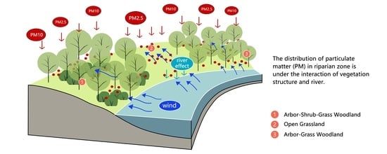
3.3.4. The Effect of the River

Although specific conclusions cannot be drawn, the river did exert some effect on the particulate removal percentages. Since the presence of trees caused changes to the particulate concentration and the removal percentage in the center of vegetation communities, to investigate the effect of the river, the observed data at 1 m and 11 m from the river were compared; these distances represent the effect of the near side and far side of the vegetation, respectively.

ANOVA revealed significant differences in the PM removal percentages and the PM_2.5/PM₁₀ ratio at a distance of 1 m and 11 m from the river (Figure 6). Figure 6a shows that the PM_2.5 removal percentage at 1 m from the river was significantly higher than that at 11 m (p < 0.001), while Figure 6b suggests the opposite for the PM₁₀ removal percentage (p < 0.001). The PM_2.5/PM₁₀ ratio provides more evidence for the effect of the river. Figure 8a shows that the PM_2.5/PM₁₀ ratio at a distance of 1 m from the river was significantly lower than that of the background (p < 0.001), as well as that at 6 m and 11 m (p < 0.05). This tendency was observed in all vegetation types. The different effect on PM_2.5 and PM₁₀ was consistent for different vegetation types and different wind conditions.

A possible cause of the change in the PM_2.5/PM₁₀ ratio is the transformation between particles of different sizes. The coagulation effect on the plant leaf surface is identified as an important mechanism for plants to remove PM [30]. This was summarized as one type of modification of PM by which the size, weight and particle number concentration of toxic PM can be changed [10]. Moreover, particulate reactions to high humidity depend on their chemical composition. Water-soluble components such as SO₄²⁻, NO³⁻, NH⁴⁺, and secondary organic matter with high hygroscopicity lead to particle growth under high humidity [41]. Therefore, the PM_2.5 at 1 m from the river was inferred to grow in size as a function of hygroscopic growth, coagulation and merging [42,43], and the coagulation effect of plant leaves was probably enhanced by the river. This likely led to a higher PM₁₀ concentration than that of the background. However, as discussed above, no significant spatial differences in the RH were observed during the observation period (Figure 5b). More data is required to verify the effect of the river and elucidate the mechanism.

4. Conclusions

Through monitoring PM_2.5 and PM₁₀ concentrations, calculating their removal efficiencies and evaluating PM_2.5/PM₁₀ ratios within three riparian plant communities, this paper found that during the monitoring period (hourly wind speed < 2.0 m/s), the open grassland (G) generally had the best removal effect, primarily due to high dispersion. However, the negative removal percentage in the middle of the vegetation community indicted the limits of open grassland. On the contrary, the obstruction effect of trees and shrubs resulted in a negative removal percentage as well as a lower concentration in the middle of the vegetation community. The result above was limited to mild-wind conditions. Different aerodynamic processes occurred under wind conditions, since the relationship between PM removal percentage and wind speed was inferred to be a discontinuous function. Compared to static situations, mild wind even decreased PM removal efficiency, causing accumulation due to laminar flow. But the large leaf surface area in the AG and the ASG also increased the impaction and interception of PM when windy. Moreover, the impact of the river on the PM_2.5 and PM₁₀ was evident at 1 m from the river, exhibiting a significantly lower ratio of PM_2.5 and PM₁₀ concentrations. This modification effect could reduce the proportion of toxic components of fine PM, and be utilized for construction of riparian open spaces beneficial for human health.

Based on the above results, two planting design schemes for urban riparian vegetation to reduce PM_2.5 and PM₁₀ exposure is recommended. First, open grassland along the river is preferred, since it not only allows for the optimization of the river’s effect, but also avoids the tree cover obstruction. Second, enough space under canopies in the middle of a woodland is recommended for leisure and activities to take full advantage of the removal effect of trees and shrubs.

It is worth noting that our study was focused only on static and mild wind conditions, and the river’s effect was only observed at 1 m from the river. The result was limited since the data selected for discussion was monitored within a limited time span under specific climate conditions and not perfectly corrected a posteriori. Therefore, long-term continuous monitoring under other weather conditions is needed in future research, especially under the conditions of higher wind speed (>2 m/s), in order to gain a more comprehensive understanding of the combined effect of vegetation structure and the river.

References

1. Kumar, P.; Druckman, A.; Gallagher, J.; Gatersleben, B.; Allison, S.; Eisenman, T.S.; Hoang, U.; Hama, S.; Tiwari, A.; Sharma, A.; et al. The nexus between air pollution, green infrastructure and human health. Environ. Int. 2019, 133, 105181. [Google Scholar] [CrossRef] [PubMed]
2. Warburton, D.E.R.; Bredin, S.S.D.; Shellington, E.M.; Cole, C.; de Faye, A.; Harris, J.; Kim, D.D.; Abelsohn, A. A Systematic Review of the Short-Term Health Effects of Air Pollution in Persons Living with Coronary Heart Disease. J. Clin. Med. 2019, 8, 274. [Google Scholar] [CrossRef] [Green Version]
3. Wu, X.; Nethery, R.C.; Sabath, M.B.; Braun, D.; Dominici, F. Air pollution and COVID-19 mortality in the United States: Strengths and limitations of an ecological regression analysis. Sci. Adv. 2020, 6, eabd4049. [Google Scholar] [CrossRef]
4. Wang, Y.; Shi, Z.; Shen, F.; Sun, J.; Huang, L.; Zhang, H.; Chen, C.; Li, T.; Hu, J. Associations of daily mortality with short-term exposure to PM2.5 and its constituents in Shanghai, China. Chemosphere 2019, 233, 879–887. [Google Scholar] [CrossRef] [PubMed]
5. Kim, K.-H.; Kabir, E.; Kabir, S. A review on the human health impact of airborne particulate matter. Environ. Int. 2015, 74, 136–143. [Google Scholar] [CrossRef]
6. Zhang, K.; Zhou, L.; Fu, Q.; Yan, L.; Morawska, L.; Jayaratne, R.; Xiu, G. Sources and vertical distribution of PM2.5 over Shanghai during the winter of 2017. Sci. Total Environ. 2020, 706, 135683. [Google Scholar] [CrossRef]
7. Völker, S.; Kistemann, T. Developing the urban blue: Comparative health responses to blue and green urban open spaces in Germany. Health Place 2015, 35, 196–205. [Google Scholar] [CrossRef]
8. Crouse, D.L.; Pinault, L.; Balram, A.; Brauer, M.; Burnett, R.T.; Martin, R.V.; van Donkelaar, A.; Villeneuve, P.J.; Weichenthal, S. Complex relationships between greenness, air pollution, and mortality in a population-based Canadian cohort. Environ. Int. 2019, 128, 292–300. [Google Scholar] [CrossRef] [PubMed]
9. Pascal, D.I.M.; Corinne, C.; Patrice, M.; Michel, V.; Yann, L.C.; Antoine, G.; Clémentine, G.; Jocelyne, P.-H.; Cyril, R.; Carolyne, V. Method for the rapid assessment and potential mitigation of the environmental effects of development actions in riparian zone. J. Environ. Manag. 2020, 276, 111187. [Google Scholar] [CrossRef]
10. Diener, A.; Mudu, P. How can vegetation protect us from air pollution? A critical review on green spaces’ mitigation abilities for air-borne particles from a public health perspective–with implications for urban planning. Sci. Total Environ. 2021, 796, 148605. [Google Scholar] [CrossRef] [PubMed]
11. Janhäll, S. Review on urban vegetation and particle air pollution–Deposition and dispersion. Atmos. Environ. 2015, 105, 130–137. [Google Scholar] [CrossRef]
12. Fowler, D.; Cape, J.N.; Unsworth, M.H.; Mayer, H.; Crowther, J.M.; Jarvis, P.G.; Gardiner, B.; Shuttleworth, W.J.; Jarvis, P.G.; Monteith, J.L.; et al. Deposition of atmospheric pollutants on forests. Philos. Trans. R. Soc. Lond. B Biol. Sci. 1989, 324, 247–265. [Google Scholar] [CrossRef]
13. Speak, A.F.; Rothwell, J.J.; Lindley, S.J.; Smith, C.L. Urban particulate pollution reduction by four species of green roof vegetation in a UK city. Atmos. Environ. 2012, 61, 283–293. [Google Scholar] [CrossRef]
14. He, C.; Qiu, K.; Alahmad, A.; Pott, R. Particulate matter capturing capacity of roadside evergreen vegetation during the winter season. Urban For. Urban Green. 2020, 48, 126510. [Google Scholar] [CrossRef]
15. Wang, L.; Gong, H.; Liao, W.; Wang, Z. Accumulation of particles on the surface of leaves during leaf expansion. Sci. Total Environ. 2015, 532, 420–434. [Google Scholar] [CrossRef]
16. Roupsard, P.; Amielh, M.; Maro, D.; Coppalle, A.; Branger, H.; Connan, O.; Laguionie, P.; Hébert, D.; Talbaut, M. Measurement in a wind tunnel of dry deposition velocities of submicron aerosol with associated turbulence onto rough and smooth urban surfaces. J. Aerosol Sci. 2013, 55, 12–24. [Google Scholar] [CrossRef] [Green Version]
17. Petroff, A.; Mailliat, A.; Amielh, M.; Anselmet, F. Aerosol dry deposition on vegetative canopies. Part I: Review of present knowledge. Atmos. Environ. 2008, 42, 3625–3653. [Google Scholar] [CrossRef]
18. Chen, X.; Pei, T.; Zhou, Z.; Teng, M.; He, L.; Luo, M.; Liu, X. Efficiency differences of roadside greenbelts with three configurations in removing coarse particles (PM10): A street scale investigation in Wuhan, China. Urban For. Urban Green. 2015, 14, 354–360. [Google Scholar] [CrossRef]
19. Lee, E.S.; Ranasinghe, D.R.; Ahangar, F.E.; Amini, S.; Mara, S.; Choi, W.; Paulson, S.; Zhu, Y. Field evaluation of vegetation and noise barriers for mitigation of near-freeway air pollution under variable wind conditions. Atmos. Environ. 2018, 175, 92–99. [Google Scholar] [CrossRef]
20. Zhang, L.; Zhang, Z.; McNulty, S.; Wang, P. The mitigation strategy of automobile generated fine particle pollutants by applying vegetation configuration in a street-canyon. J. Clean. Prod. 2020, 274, 122941. [Google Scholar] [CrossRef]
21. Zhu, D.; Gillies, J.A.; Etyemezian, V.; Nikolich, G.; Shaw, W.J. Evaluation of the surface roughness effect on suspended particle deposition near unpaved roads. Atmos. Environ. 2015, 122, 541–551. [Google Scholar] [CrossRef]
22. Baldauf, R. Roadside vegetation design characteristics that can improve local, near-road air quality. Transp. Res. Part D Transp. Environ. 2017, 52, 354–361. [Google Scholar] [CrossRef]
23. Bowker, G.E.; Baldauf, R.; Isakov, V.; Khlystov, A.; Petersen, W. The effects of roadside structures on the transport and dispersion of ultrafine particles from highways. Atmos. Environ. 2007, 41, 8128–8139. [Google Scholar] [CrossRef]
24. Jeanjean, A.P.R.; Monks, P.S.; Leigh, R.J. Modelling the effectiveness of urban trees and grass on PM2.5 reduction via dispersion and deposition at a city scale. Atmos. Environ. 2016, 147, 1–10. [Google Scholar] [CrossRef] [Green Version]
25. Chen, L.; Liu, C.; Zou, R.; Yang, M.; Zhang, Z. Experimental examination of effectiveness of vegetation as bio-filter of particulate matters in the urban environment. Environ. Pollut. 2016, 208, 198–208. [Google Scholar] [CrossRef]
26. Chen, X.; Wang, X.; Wu, X.; Guo, J.; Zhou, Z. Influence of roadside vegetation barriers on air quality inside urban street canyons. Urban For. Urban Green. 2021, 63, 127219. [Google Scholar] [CrossRef]
27. Abhijith, K.V.; Kumar, P.; Gallagher, J.; McNabola, A.; Baldauf, R.; Pilla, F.; Broderick, B.; Di Sabatino, S.; Pulvirenti, B. Air pollution abatement performances of green infrastructure in open road and built-up street canyon environments—A review. Atmos. Environ. 2017, 162, 71–86. [Google Scholar] [CrossRef]
28. Frank, C.; Ruck, B. Numerical study of the airflow over forest clearings. For. Int. J. For. Res. 2008, 81, 259–277. [Google Scholar] [CrossRef] [Green Version]
29. Xing, Y.; Brimblecombe, P. Role of vegetation in deposition and dispersion of air pollution in urban parks. Atmos. Environ. 2019, 201, 73–83. [Google Scholar] [CrossRef]
30. Yin, S.; Lyu, J.; Zhang, X.; Han, Y.; Zhu, Y.; Sun, N.; Sun, W.; Liu, C. Coagulation effect of aero submicron particles on plant leaves: Measuring methods and potential mechanisms. Environ. Pollut. 2020, 257, 113611. [Google Scholar] [CrossRef] [PubMed]
31. Liu, J.; Zhu, L.; Wang, H.; Yang, Y.; Liu, J.; Qiu, D.; Ma, W.; Zhang, Z.; Liu, J. Dry deposition of particulate matter at an urban forest, wetland and lake surface in Beijing. Atmos. Environ. 2016, 125, 178–187. [Google Scholar] [CrossRef]
32. Anda, A.; Soos, G.; Teixeira da Silva, J.A.; Kozma-Bognar, V. Regional evapotranspiration from a wetland in Central Europe, in a 16-year period without human intervention. Agric. For. Meteorol. 2015, 205, 60–72. [Google Scholar] [CrossRef]
33. Du, H.; Song, X.; Jiang, H.; Kan, Z.; Wang, Z.; Cai, Y. Research on the cooling island effects of water body: A case study of Shanghai, China. Ecol. Indic. 2016, 67, 31–38. [Google Scholar] [CrossRef]
34. Xuan, C.Y.; Wang, X.Y.; Jiang, W.M.; Wang, Y.W. Impacts of water layout on the atmospheric environment in urban areas. Meteorol. Mon. 2010, 36, 94–101. (In Chinese) [Google Scholar]
35. Wu, F.F.; Zhang, N.; Chen, X.Y. Effects of riparian buffers of North Mort of Beijing on air temperature and relative humidity. Acta Ecol. Sin. 2013, 33, 2292–2303. (In Chinese) [Google Scholar]
36. Xing, Y.; Brimblecombe, P. Dispersion of traffic derived air pollutants into urban parks. Sci. Total Environ. 2018, 622–623, 576–583. [Google Scholar] [CrossRef]
37. Zhang, L.H.; Li, S.H. Research on the influence of urban water bodies on temperature and humidity of surrounding green spaces in the horizontal direction. In Proceedings of the Beijing Symposium on “Building Conservation Oriented Landscaping”, Beijing, China, 1 October 2007; p. 10. (In Chinese). [Google Scholar]
38. Han, D.; Shen, H.; Duan, W.; Chen, L. A review on particulate matter removal capacity by urban forests at different scales. Urban For. Urban Green. 2020, 48, 126565. [Google Scholar] [CrossRef]
39. Zhang, L.; Zhang, Z.; Feng, C.; Tian, M.; Gao, Y. Impact of various vegetation configurations on traffic fine particle pollutants in a street canyon for different wind regimes. Sci. Total Environ. 2021, 789, 147960. [Google Scholar] [CrossRef]
40. Qiu, L.; Liu, F.; Zhang, X.; Gao, T. The reducing effect of green spaces with different vegetation structure on atmospheric particulate matter concentration in BaoJi City, China. Atmosphere 2018, 9, 332. [Google Scholar] [CrossRef] [Green Version]
41. Sun, Y.; He, Y.; Kuang, Y.; Xu, W.; Song, S.; Ma, N.; Tao, J.; Cheng, P.; Wu, C.; Su, H.; et al. Chemical Differences Between PM1 and PM2.5 in Highly Polluted Environment and Implications in Air Pollution Studies. Geophys. Res. Lett. 2020, 47, e2019GL086288. [Google Scholar] [CrossRef]
42. Zhu, Y.; Hinds, W.C.; Kim, S.; Sioutas, C. Concentration and Size Distribution of Ultrafine Particles Near a Major Highway. J. Air Waste Manag. Assoc. 2002, 52, 1032–1042. [Google Scholar] [CrossRef] [PubMed]
43. Zhu, C.; Zeng, Y. Effects of urban lake wetlands on the spatial and temporal distribution of air PM10 and PM2.5 in the spring in Wuhan. Urban For. Urban Green. 2018, 31, 142–156. [Google Scholar] [CrossRef]
Figure 1. (a) The location of the sampling sites in Shanghai, China; (b) the locations of three sampling sites in the campus of Shanghai Jiao Tong University, Minhang district; the instrumentation locations of measuring stations beside the Danshui River in three vegetation types: (c) arbor-shrub-grass woodland (ASG), (d) open grassland (G) and (e) arbor-grass woodland (AG); the instrumentation locations and heights of measuring stations in three vegetation types: (f) arbor-shrub-grass woodland (ASG), (g) open grassland (G) and (h) arbor-grass woodland (AG).
Atmosphere 12 01428 g001
Figure 2. (a) Hourly trends in the average PM2.5 and PM10 concentrations within the three vegetation types: open grassland (G), arbor-grass woodland (AG) and arbor-shrub-grass woodland (ASG); (b) ANOVA results for the PM2.5 and PM10 concentrations in different vegetation types and distances from the river across the entire observation period. ** p ≤ 0.01; Error bar: standard deviation.
Atmosphere 12 01428 g002
Figure 3. Results of the cluster analysis of the PM2.5 and PM10 spatial distributions across time. (a) Spatial-temporal distribution of the PM2.5 and PM10 concentrations in (i) grassland (G); (ii) arbor-grass (AG) woodland; (iii) arbor-shrub-grass (ASG) woodland generated using hourly data points at the distances of 1 m, 6 m, and 11 m from the river. (b) The distribution across time of five clusters in (i) grassland (G); (ii) arbor-grass (AG) woodland; (iii) arbor-shrub-grass (ASG) woodland as a result of the hierarchical cluster analysis. (c) The spatial-temporal distribution of PM2.5 and PM10 in the background atmosphere at 10 m above ground. (d) The average PM2.5 and PM10 concentrations at the stepped distance of the five clusters based on the hierarchical cluster analysis.
Atmosphere 12 01428 g003
Figure 4. (a) Hourly trends in all three types of vegetation at (i) 1 m, (ii) 6 m, and (iii) 11 m distances from the river. (b) The spatial-temporal distribution of the removal percentages of the PM2.5 and PM10 in: (i) grassland (G); (ii) arbor-grass (AG) woodland; (iii) arbor-shrub-grass (ASG) woodland. (c) The spatial-temporal distribution of the wind speed in (i) grassland (G), (ii) arbor-grass (AG) woodland, and (iii) arbor-shrub-grass (ASG) woodland.
Atmosphere 12 01428 g004
Figure 5. ANOVA results of the (a) wind speed, (b) relative humidity (RH), and (c) temperature in different vegetation types and distances from the river across the entire observation period. ** p ≤ 0.01 *** p ≤ 0.001; Error bar: standard deviation; G: open grassland; AG: arbor-grass woodland; ASG: arbor-shrub-grass woodland.
Atmosphere 12 01428 g005
Figure 6. ANOVA results of (a) the PM2.5 removal percentage and (b) the PM10 removal percentage during the entire observation period; ANOVA results of (c) the PM2.5 removal percentage and (d) the PM10 removal percentage during mild-wind and static periods, respectively. * p ≤ 0.05 ** p ≤ 0.01 *** p ≤ 0.001. Error bar: standard deviation; G: open grassland; AG: arbor-grass woodland; ASG: arbor-shrub-grass woodland.
Atmosphere 12 01428 g006
Figure 7. Scatter plots of all the data points during mild-wind periods from all vegetation types: (a) wind speeds and PM2.5 removal percentages, (b) wind speeds and PM10 removal percentages. Scatter plots of the data points during mild-wind periods for different vegetation types separately: (c) wind speeds and PM2.5 removal percentages, (d) wind speeds and PM10 removal percentages. G: open grassland; AG: arbor-grass woodland; ASG: arbor-shrub-grass woodland.
Atmosphere 12 01428 g007
Figure 8. ANOVA results of the PM2.5/PM10 ratio in different vegetation types and distances: (a) during the entire observation period, (b) under static conditions, and (c) under mild-wind conditions. * p ≤ 0.05 ** p ≤ 0.01 *** p ≤ 0.001. Error bar: standard deviation; G: open grassland; AG: arbor-grass woodland; ASG: arbor-shrub-grass woodland.
Atmosphere 12 01428 g008