Article

Impact of Climate Variability on Climate Beach-Based Tourism Aptitude: A Case Study in the Atlantic Coast of SW Europe

by
Domingo F. Rasilla
Departamento de Geografía, Urbanismo y Ordenación del Territorio, Universidad de Cantabria, 39005 Santander, Spain
Atmosphere 2021, 12(10), 1328; https://doi.org/10.3390/atmos12101328
Submission received: 31 August 2021 / Revised: 30 September 2021 / Accepted: 6 October 2021 / Published: 12 October 2021
(This article belongs to the Section Biometeorology)

Abstract

:
The spatial and temporal variability of the summer (July–August) climate beach-based tourism aptitude along the Atlantic coast of SW Europe from 1973 to 2017 and its links with the atmospheric circulation has been analyzed, combining an empirical index and a circulation pattern approach. Three different coastal sectors were defined from a PCA analysis: Galicia-N of Portugal, the Gulf of Biscay, and the western coast of France and the English Channel. Each region experienced a contrasted evolution due to geographical factors such as latitude, orography and exposure to the prevailing circulation patterns. No significant increase in aptitude was found because the background warming has not been balanced by trends in cloudiness or precipitation. Several possible causes are discussed, from local to large-scale, such as the recent evolution of the summer NAO pattern impacting the northernmost region.

Graphical Abstract

1. Introduction

Research on Applied Climatology has focused on two main lines: one envisages the atmosphere as a risk system capable of endangering the natural environment and human activities, while for the other, the atmosphere is a natural resource for human development [1]. Tourism Climatology is included within the latter.
Tourism has become one of the most important economic activities in many countries and has been under continuous expansion over the past several decades, playing a relevant role in promoting the development of national economies [2]. Although there are multiple factors explaining the diversity of touristic activities, it is no less true that weather and climate resources play a relevant role on specific typologies.
Climate is undoubtedly the most important resource for most 3S (sand, sea, and sun) destinations. It directly drives the main intra- and interregional travel flows (mostly from temperate to subtropical and tropical regions), significantly influencing the number of visits [3]. Moreover, climate also regulates other natural assets, such as beach environments, land- and seascapes or regional biodiversity, supplementary natural resources which are additional attraction factors that improve the visitor’s satisfaction levels.
Unlike “climate-dependent” destinations, such as the Mediterranean, ‘weather-sensitive’ destinations are those in which climate is not a tourist resource itself. According to Smith’s scheme [4,5], beach visitors in ‘weather sensitive’ destinations used to accommodate their activities to the variable daily weather conditions; most of them could be categorized as ‘day-trippers’, i.e., they reside relatively close to the coast, visiting beaches if the weather meets their expectations, but shifting to alternative activities otherwise. Flexibility to adapt plans and opportunism to take advantage of weather conditions for bathing are key concepts for those visitors. The Atlantic seaboard of southwestern Europe can be included well into the category of “weather-sensitive” beach destinations because beach attendance is linked to clear skies and the lack of rainfall [6,7,8,9,10]. The region includes several resorts (e.g., La Toja, Santander and San Sebastian in Spain; Biarritz, Ille of Ré in France; and Brighton in the UK) whose long touristic traditions, linked to the “sea bathing” therapies among wealthiest, goes back to the middle of the 19th century. Despite a lower volume of visitors in comparison with the Mediterranean coast, tourism represents an important income source for those regional economies and evidence differentiating features. For example, 87% of the visitors who arrive to Cantabria (N. Spain) are domestic travelers, mostly as familiar units, spending no more than a week and using housing renting, camping or rural hotels [11].
Movement restrictions between countries caused by COVID-19 drastically interrupted international travel, causing massive drops in the arrival of tourists to the main international 3S destinations. In return, movements to domestic destinations increased substantially. Despite the progressive easing of travel restrictions, a return to pre-pandemic conditions does not seem likely, at least in the coming years [12,13]. Images of July 2020, when an anomalous hot and dry period took place across Western Europe, showed crowded beaches on the SE coast of the UK and NW France, traffic jams, water supply difficulties in locations of Northern Spain, etc. These problems can be considered a good preview of future scenarios linked to the increase in global temperatures. Studies focused on tourism activities and climate change advise of a deterioration of the future climatic conditions during the current peak demand season in the Mediterranean, whereas improving in central and northern Europe [14,15,16,17,18]. Tourists coming from the latter regions may not travel so far if enjoying more appealing summer climatic conditions at home, thus preferring domestic rather than Mediterranean emplacements. Thus, changes in the length, seasonality, and quality of the resource for highly dependent climate tourist activities (i.e., beach-based tourism) could have important implications for competitive relationships among destinations and their profitability, and the potential consequences of climate change may be relevant not only in the destination countries, but also in countries of origin [19,20,21,22]. Moreover, such massive inflow of visitors might potentially impact severely different natural and human activities upon coastal areas which have not experienced the same human pressure suffered by the Mediterranean coasts.
In the context of climate beach-based tourism studies, the aptitude of a destination to meet the weather expectations of beach users can be evaluated through climate indices. It appears that Mieczkowski’s Tourism Climate Index (TCI) is still the most applied empirical index in multiple destinations and tourist segments [23]. Despite successive adaptations for beach tourism (e.g., Beach Climate Index—BCI—[24]; Modified Climate Index for Tourism—MCIT—[25]), none of them have not been tested from declared or revealed preferences. To overcome that deficiency, the Holiday Climate Index from 3S tourism (HCI: Beach; [26,27]) has been designed specifically to evaluate the recreational beach segment. The HCI: Beach integrates the thermal, physical, and aesthetic facets of the climatic variables relevant for this kind of tourism segment [28], its calculation is simple, and it has been tested empirically. It also recognizes the non-linear impact of certain variables on beach attendance, since both declared and stated preference studies emphasize clear skies and the lack of rain as the best weather conditions for beach attendance [8,9,10,29,30,31]. Therefore, the HCI: Beach also includes a penalizing function to account the overriding role of variables such as rain and wind speed. In addition, it assumes higher thermal thresholds, due to the resilience of bathers to conditions that could be classified as thermal stress in other activities [32,33]. The HCI: Beach has been applied to different destinations and climatic settings, to characterize both current and future conditions [34,35,36]. However, to date, the HCI: Beach index has not been used to assess its long-term variability or its links with atmospheric circulation, unlike other bioclimatic indices [37,38,39,40,41,42]. Characterizing the climate beach-based tourism aptitude on a regional-scale basis, as observed in the instrumental record, is a necessary initial step toward making meaningful assessments of the accuracy of regional climate predictions. Furthermore, a process-based understanding of the causes of low-frequency variability in regional climates may improve future medium- to long-range regional forecasting capabilities. Additionally, the study of the interannual variability and trends is important in the context of the ongoing climatic change, which may significantly affect the frequency and duration of specific weather conditions, favorable to the development of a given leisure activity.
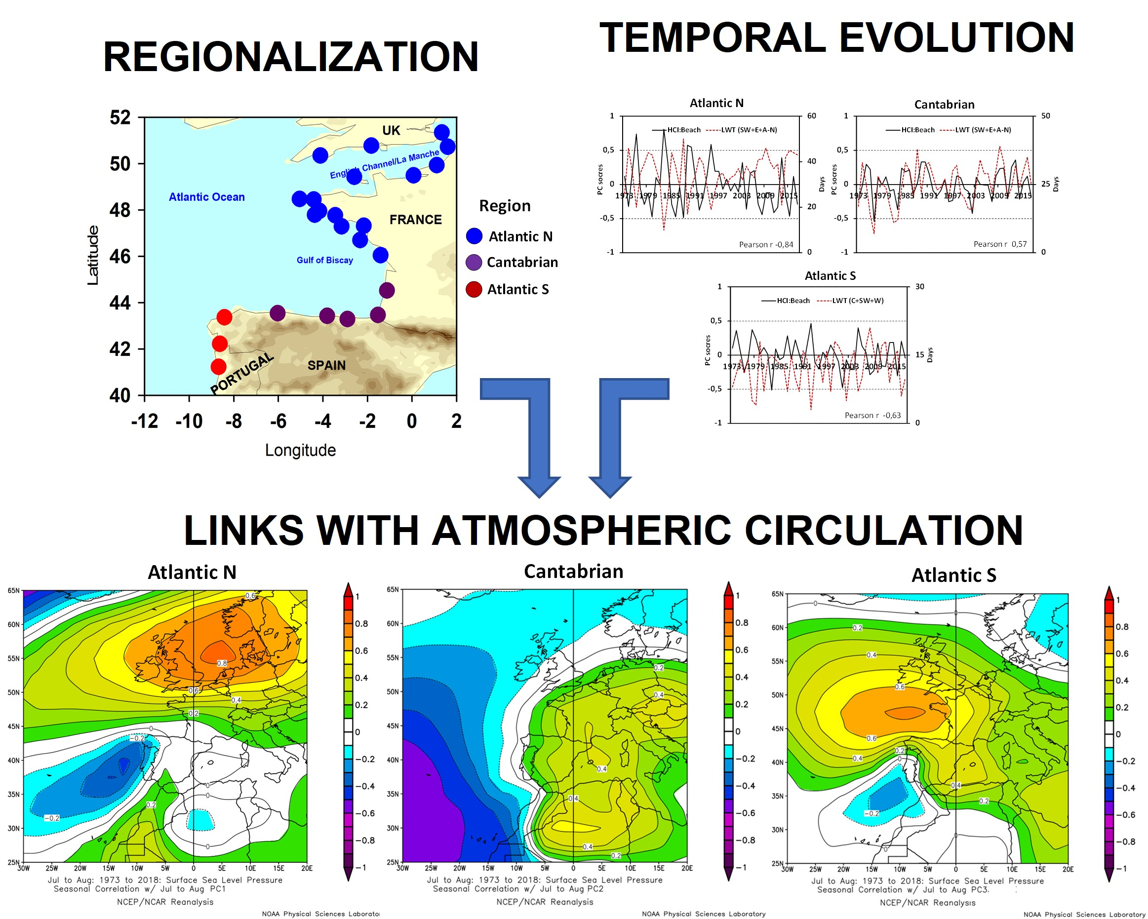
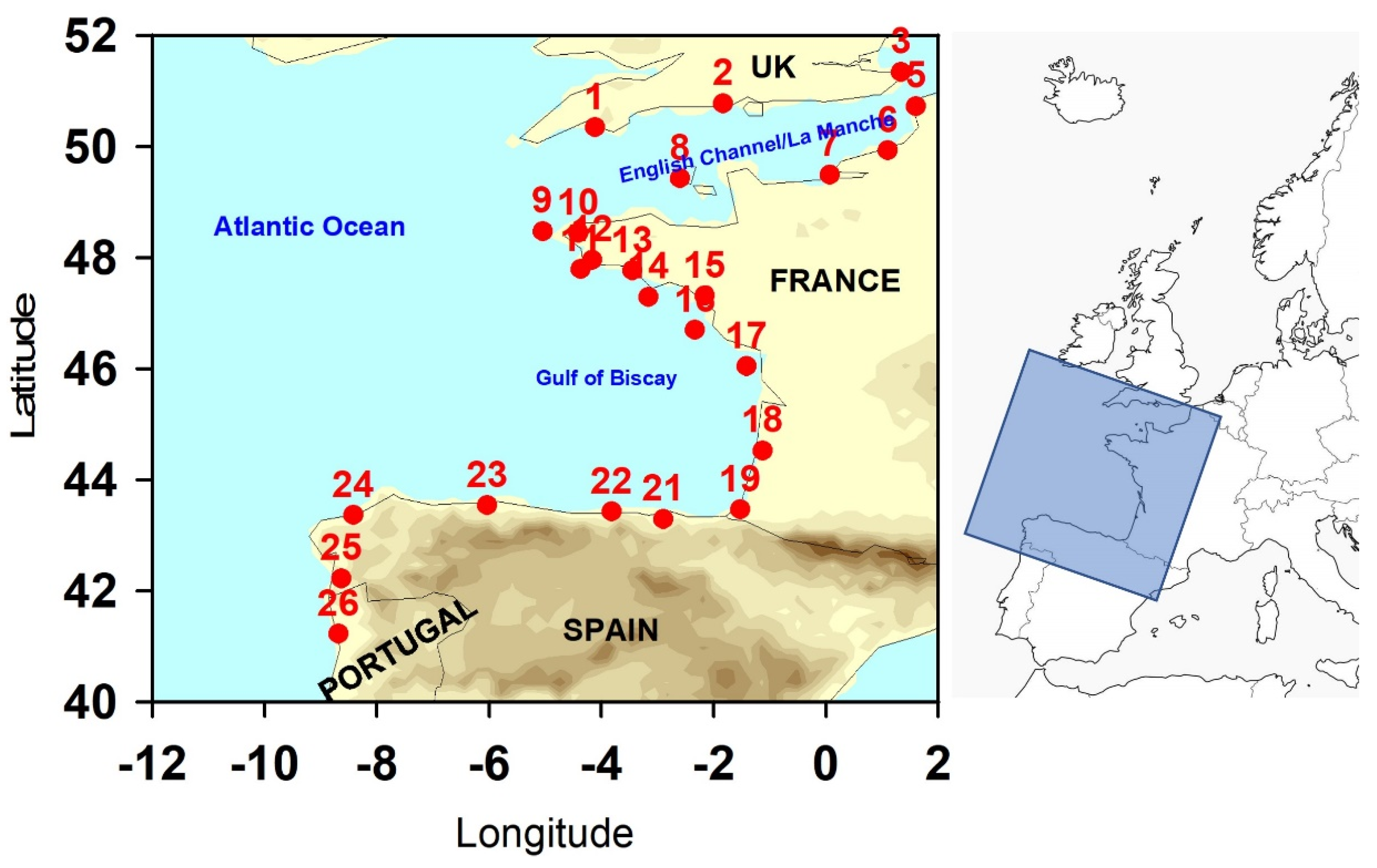
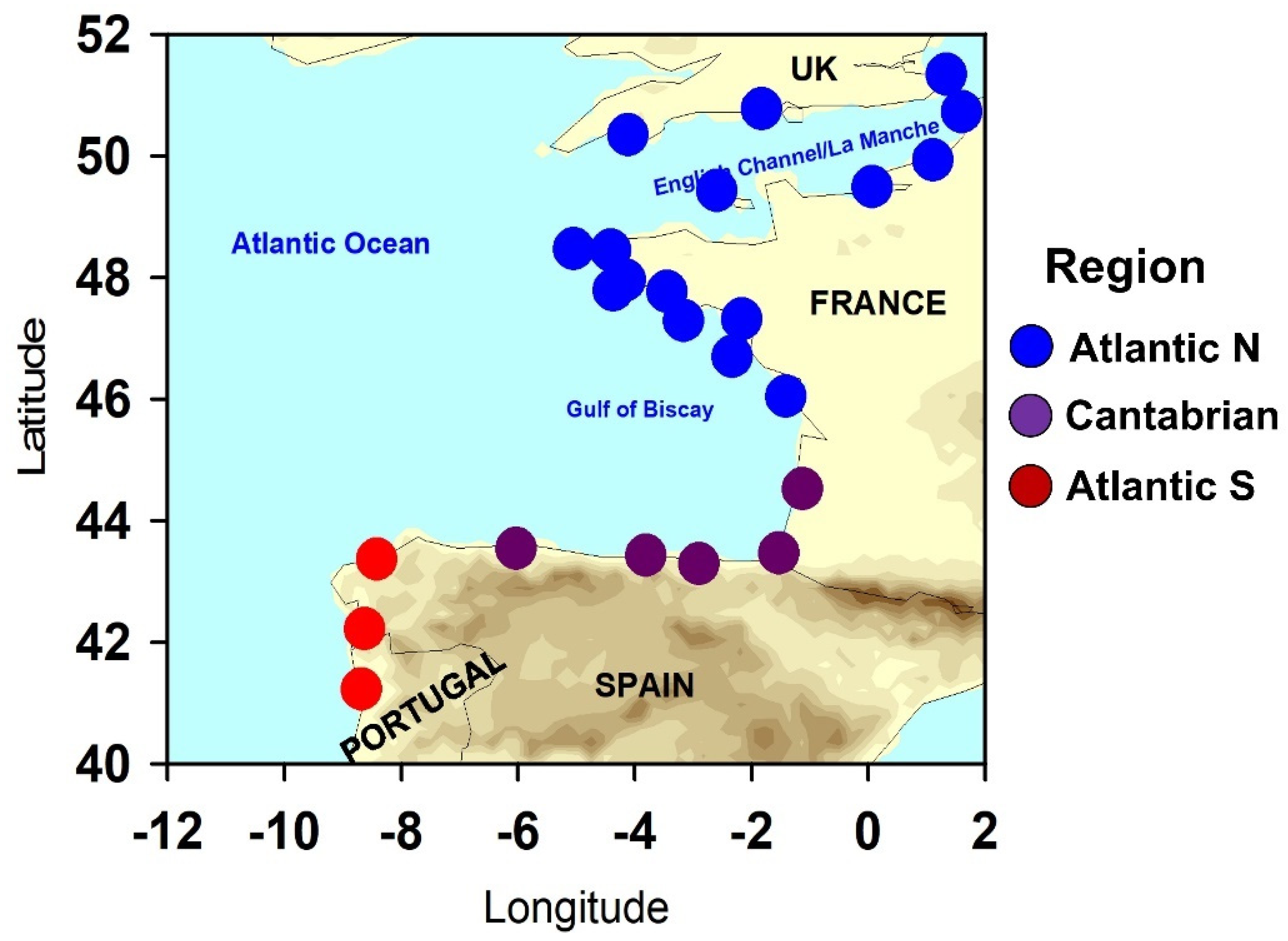
Consequently, the main objective of this contribution is to analyze the current climate beach-based tourism aptitude along the Atlantic Coast of SW Europe and its recent decadal evolution using the HCI: Beach index. With such an objective in mind, (1) the main spatial and temporal features are described; (2) its temporal evolution since 1973 till 2017 is analyzed and (3) linked with the recent evolution of the atmospheric circulation at different scales.

2. Materials and Methods

2.1. Materials

This research is based on the calculation of daily HCI: Beach index values from the period 1973 to 2017 derived separately from 26 synoptic stations (Figure 1). The national meteorological networks of the UK, France, Spain and Portugal were screened for stations which accomplished the following criteria: almost complete records (less than 5% of missing data were allowed), a distance not exceeding 10 km from the coast and no higher than 150 m above sea level (except in the case of Vigo-Peinador airport, on the western coast of Galicia). The source of the data was the Met Office Integrated Data Archive System (MIDAS) Land and Marine Surface Stations Data (1853–current) for UK data [43], the French Meteorological Service (MeteoFrance) in the case of France and the Integrated Surface Database (ISD) for Spain and Portugal data [44]. Regarding homogeneity issues, annual time series of each variable were submitted to detect change points using the Standard Normal Homogeinity Test (SNHT), included in the “Trends” R package [45], finding no significative breaks, although some concerns arise regarding cloud cover in UK due to the replacement of human observations by ceilometers (UKMO, personal communication).
NCEP/NCAR reanalysis data for the same period of surface meteorological data were used [46] to extract composites of sea level pressure fields through the web site application (https://psl.noaa.gov/data/composites/day/, accessed on 31 August 2021).
Seasonal indices of major teleconnection patters (NAO, EA and SCAND) were downloaded from the Climate Prediction Center web site (https://www.cpc.ncep.noaa.gov/data/teledoc/telecontents.shtml, accessed on 31 August 2021).

2.2. Methods

The HCI: Beach [26,27] uses five weather variables (temperature, humidity, cloud cover, precipitation, and wind speed) to derive three sub-indices accounting for the thermal, aesthetic, and physical dimensions of climate relevant to tourism. HCI: Beach is calculated as:
HCI: Beach = 2(TC) + 4(A) + 3(P) + W
where TC is thermal comfort (combination of the maximum and mean relative humidity) and has a 20% weight; A is the aesthetic dimension (cloud cover %), weighting 40%; P is precipitation with a 30% weight; and W is windspeed with a 10% weight. A more detailed explanation of the procedure, weights and ratings can be found in Appendix B.
Principal Component Analysis (PCA) was used to analyze the spatio-temporal variability of the HCI: Beach index across the study region [47,48]. The aim of PCA is to create a new set of uncorrelated variables that are a linear combination of the initial variables and explain as much of the initial variation as possible. Several subjective choices by the researcher can potentially affect the outcome of a PCA. The input data were organized into a S-mode of decomposition (days as rows and corresponding values of HCI: Beach on each meteorological station as columns), and the covariance matrix was preferred since it portrays more accurately the data’s spatial variability; in addition, the data are measured in the same units. The election of the number of significant Principal Components was based on the break point of the scree plot, a graph depicting the explained variance corresponding to each component. Two outcomes of the PCA are useful for the purposes of this research: the component-loadings matrix and the component-scores matrix. The first matrix depicts the strength of each spatial mode of variability on each meteorological station, while the component scores matrix contains the projection of the intensity of each component on time. Relationships between original variables and the new components are not always clear, so rotation can facilitate which original variables load most highly on which component. The orthogonal VARIMAX rotation was used to better delimitate the boundaries between spatial units [49].
Sea level pressure patterns were categorized using the Lamb Weather Type (henceforth LWT, [50]) objective classification scheme. Airflow properties, derived from a 5° by 10° latitude-longitude grid array and computed from 12 UTC daily SLP values are classified using three basic variables that define circulation features over the study area: the direction of mean flow (D), the strength of mean flow (F) and the vorticity (Z). A set of daily index values are calculated using the equations in Appendix C. The final catalogue consists of eight pure advective (or directional) types based on wind direction (e.g., W, NW, N and so on); A and C types, which represent anticyclonic and cyclonic pressure patterns, respectively, but no coherent flow direction, and an undetermined (U) type, which represents patterns that have weak pressure gradients, and thus neither flow direction nor vorticity can be identified. Procedure to calculate the different LWTs and a composite of each type are displayed in Appendix C.
Detection and estimation of trends in time series was accomplished through the nonparametric Mann-Kendall and Theil-Sen’s methods. The first test is applicable to the detection of a monotonic trend of a time series, while the second fits a linear model for the trend, also included in the R Package “Trends”.
Finally, links between variables were explored through correlation (Pearson´s Correlation Coefficient) analysis. For example, correlation maps between temporal indices HCI: Beach and Sea Level Pressure were used to confirm the impact of large-scale circulation patterns.

3. Results

3.1. General Features of Climate Beach-Based Tourism Aptitude in the SW Europe Atlantic Seabord

The study area enjoys a humid oceanic climate (Csb or Cfb) characterized by moderate thermal amplitudes, frequent precipitation, and abundant cloudiness. Figure 2a displays the annual regime of the HCI: Beach index in some selected locations. Besides an expected latitudinal gradient, a clear seasonal cycle is revealed, with maximum values during summer (July or August) and minimum in winter. The bell-shaped profile, typical of the mid-latitude temperate climates, as opposed to the twin maxima characteristic of warmer climates, is not exactly symmetrical. The transition between the summer maximum and the winter minimum is more abrupt than the spring recovery, probably because of the sea surface temperatures. It is interesting to note the singularity of the Cantabrian Coast (Santander), which shows lower aptitude than, e.g., St. Nazaire, placed more northerly, from April to October. Consequently, the research will focus on the bimester July and August, also the moment of the year coinciding with official vacations.
Table 1 shows the Pearson Correlation Coefficient between latitude and several meteorological variables and derived indices. Thermal variables (temperature and Humidex) show an expected negative strong relationship with latitude, because of differences on radiation and heat budget. Cloud cover and wind speed show positive links with latitude, in this case related to the proximity to the main Atlantic storm track. Similar explanation justifies the negative relationship with the frequency of wet days, while no significant relationship is observed with relative humidity and precipitation.
Figure 2b displays the spatial anomalies of the summer (July–August) HCI: Beach regressed against latitude. This procedure highlights areas in which the values are higher than expected due to their latitudinal location, and areas in which said index has a value below the predicted by the statistical model. The SE coast of Great Britain (except Plymouth), the entire Atlantic coast of France south to Brittany and the coast of Galicia and Portugal display positive anomalies. On the contrary, negative ones are concentrated on the French coast of the English Channel, particularly in its westernmost extreme (Brittany) and the Northern coast of the Iberian Peninsula. Note that coasts with positive anomalies are orientated to the W or SW (or S in the case of UK) while coasts with negative anomalies faced northward.

3.2. Regionalization of Summer Climate Beach-Based Tourism Aptitude

The evidence of a similar behavior among nearby observatories supports an additional analysis to precisely identify which stations follow similar interannual variations of climate beach-based tourism aptitude, followed by an analysis of their long-term trends. July–August (J-A) daily HCI: Beach indices variability was primarily captured by three RPCs. Each one represents a spatial area with a coherent temporal evolution. The loading vectors (spatial patterns) for these RPCs are presented in Figure 3, with the value at station equal to the correlation coefficient between original time series and the RPC. The first Principal Component (henceforth Atlantic N region) accounts for 47% of the spatial variance and groups all stations located northward the 45° parallel (France and UK). The second component (Cantabrian region) represents an additional 18% of the original variability, and groups the Spanish meteorological observatories places along the Cantabrian Coast, plus Biarritz and Cazaux, in southwestern France. The last component (Atlantic S region), representing 9% of the variance, loads the most along the Atlantic coast of Spain and Portugal.
The rotated Principal Components scores represent temporal indices of interannual variability of regional climate. To facilitate their evaluation, the original daily time series were averaged into seasonal (July–August) values, and then submitted to a further analysis to detect and estimate trends in time. Nevertheless, none of time series displays any significant upward or downward trends (Table 2); some temporal features are however noteworthy and will be discussed in more detail later.

3.3. Regional-Scale Atmospheric Circulation Variability and Climate Beach-Based Tourism Aptitude

Once the spatial variability in climate beach-based tourism aptitude has been analyzed, this section deals with the atmospheric circulation mechanisms supporting the previous findings, and how those mechanisms shape the long-term interannual variability on climate aptitude. Figure 4 shows the within-group variance of daily Principal Component scores for each of the eleven synoptic categories and three regions. Values above 0 indicate an LWT prone to high values of the HCI: Beach index; the opposite is true for values below 0. In general, there is a common agreement regarding the types favorable/unfavorable; what is not similar is the value of the anomaly.
Thus, a one-way analysis of variance (ANOVA) was undertaken to determine whether the mean values of the Principal Component scores within the synoptic categories were significantly different. Results rejected the null hypothesis that all category means were equal at the three regions (Table 3). As there was a statistically significant difference in mean values across the synoptic categories, a multiple comparisons method was used to identify which categories were significantly different, using the Tukey–Kramer multiple comparisons method. This method of multiple comparisons was chosen for its aptitude in analyses involving uneven sample sizes because there were different numbers of days falling within each synoptic category.
The Table 3 includes which LWTs on each region are the most different, becoming candidates to explain the anomalous temporal behavior of the Principal Component scores. In order to further investigate the relationship between regional climate aptitude and LWTs on a seasonal basis, we compare, on the one hand, the long-term variability of HCI: Beach index at the three regions (represented by the seasonal averages of daily PC scores) and, on the other hand, the combined frequency of circulation patterns that were shown to be related significant values of HCI: Beach index, on each region, as obtained from the previous analysis. The results are displayed in Figure 5 and reveal a distinctive degree of association between these time series through the whole territory, with correlation coefficients between 0.84 and 0.57, all statistically significant at the 99% confidence level. The seasonal series typically show a relatively stable long-term mean, although with some decadal variability. For example, summers during the 70s and 80s were very variable in UK and northern France; very favorable summers (1976, 1983 or 1990) stand out, corresponding to long “heat waves”. Note that the infamous 2003 summer was not as extreme as the previously cited. After the year 2000, unfavorable summers predominate, such as 2009, 2012, 2013 or 2015.
Interannual variability is less evident southward, although contrasted summers do exist. Very good summers correspond to years 1989, 1990 and 2013 along the Cantabrian coast, concurrent to severe drought conditions; on the contrary, 1977, 2002 and 1983 (the same summer of one of the most severe contemporary flooding in the city of Bilbao) are examples of unfavorable summers. Equally, the coast of Galicia-N Portugal experienced several favorable/unfavorable summers; some of the former coincided with dry spells and high wildfire activity (for example, 1978).

3.4. Large-Scale Circulation Patterns

Here, the previous analysis is extended through examination of the large-scale flow regimes responsible for significantly anomalous seasons. For that task, correlations between seasonal (July and August) averages of four well-known teleconnection indices affecting the Euro-Atlantic area (NAO, EA, EA_WR and SCAND) and the average values of PC scores in each region were computed.
According with the results of Table 4, only the climate beach-based tourism aptitude of the Atlantic N region is significatively correlated with the summer NAO and EA teleconnection patterns.
A better understanding of the dynamic mechanisms underlying the previous correlations can be obtained by correlating the time series of the Principal Component scores of each region and SLP fields (Figure 6). The latitudinal structure of the spatial patterns corresponding to the regions Atlantic N and Atlantic S are closely similar since the map is dominated by broad positive correlations to the north and a tongue of negative correlations off the western coast of the Iberian Peninsula. However, the size and values of the significant correlations is much higher in the Atlantic N region. Thus, seasons with higher-than-average aptitude corresponds to higher-than-normal pressure values over the North Sea, accompanied by an intensification of the Saharan thermal low west of the Iberian Peninsula. The positive values of the correlation can be interpreted as resulting of a SW-NE movement of the Azores High, further northward of its climatological position. The spatial structure of positive and negative correlation centers shows a large resemblance with the spatial pattern of the North Atlantic oscillation in summer, confirming results from Table 4. The North Atlantic Oscillation (NAO) has been considered the most important pattern of large-scale variability for interpreting climate variability in the North Atlantic European sector, as expressed by changes in westerly winds, storminess, and surface climate parameters such as temperatures and precipitation. In comparison with its winter counterpart, the nodes of the summer NAO occupy a more northerly position and smaller spatial extent.
The structure of the spatial pattern of the Atlantic S region is similar, but the positive area is displaced southward to the Gulf of Biscay area, and the value of the correlation is substantially low.
The weakest pattern of correlation corresponds to the Cantabrian region, which even replace the zonal pattern of anomalies by a meridional one. This pattern displays a negative node of correlations in the middle of the Atlantic and a positive node over Western Europe and the Mediterranean Basin, but correlations are the lowest.

4. Discussion

The climate aptitude for beach-based tourism along the Atlantic coast of SW Europe has experienced variations in time and space during the period 1973–2017. That variability has been studied using a state-of-the-art climate tourism index; the HCI: Beach index, which considers the different climatic facets of the tourist activity and the constraining impact of specific variables, has been used.
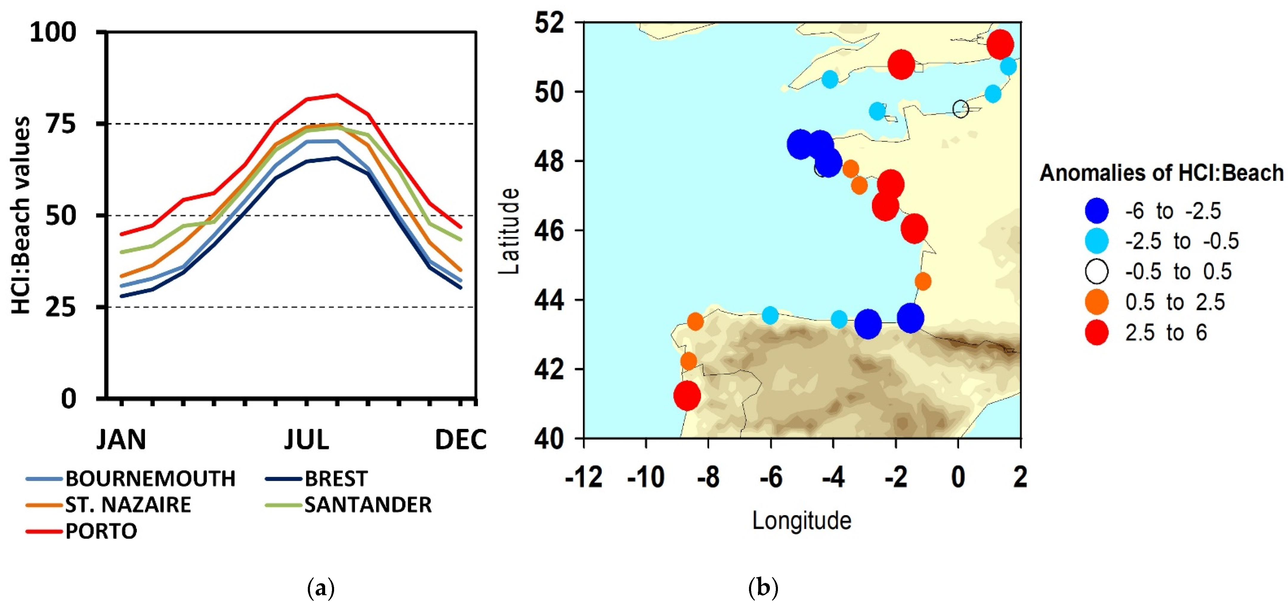
The spatial distribution of the summer values (July and August) shows a pattern controlled by latitude, although regional anomalies exist, related to the orientation of the coast regarding the prevailing circulation patterns and the presence of mountains near the coast. Thermal variables show the closest links with latitude, as result of the differences on solar radiation reception and surface heat budget. Additionally, physical variables such as wind speed and frequency of precipitation also display a significant correlation with latitude since the proximity to the main Atlantic storm track favors a greater frequency of frontal systems. Cloudiness and total precipitation, the two variables with greater weight on HCI: Beach index, do not show the same clear spatial pattern, because orography and warm sea surface temperatures tend to intensify precipitation. Consequently, that overall pattern shows distortions at various points. For example, along the English Channel, climate tourist aptitude rapidly changes from W to E, from minimum values in Cornwall/Brittany and to a maximum in Kent/Cote d’Opal. A dissymmetry is also observed between the UK and the French sides since most of the positive anomalies appear in the former. Frontal systems linked to storms crossing well above the 55° N parallel (W, NW and A LWTs) experience a progressive weakening towards the E during its eastward progression, placing the UK coast on the leeward and the French coast on the windward.
Another singularity is found in the Gulf of Biscay area, encompassing the Cantabrian and Aquitanian coasts. Due to the proximity of the Cantabrian Range and Pyrenees to the coastline, orographic cloudiness is very common in this area, even under stable atmospheric conditions, being capable of reducing the overall values of the HCI: Beach index. In addition, the development of a summer warm SST pool in the SE corner of the Gulf of Biscay provides abundant latent heat to the lower layers of the atmosphere, which, in conjunction with upper-level lows, generates convective episodes of intense rainfall events [51].
On the contrary, positive anomalies are observed across the western French coast (departments of Loire-Atlantique, Vendeé and Charente-Maritime), as well as along Galicia and Northern Portugal. The lack of any kind of topographical obstacle, beyond the own coast, in the first case, and the upwelling phenomenon in the second, explain the predominance of sunnier, drier, and warmer conditions, and, consequently, the higher values of HCI: Beach.
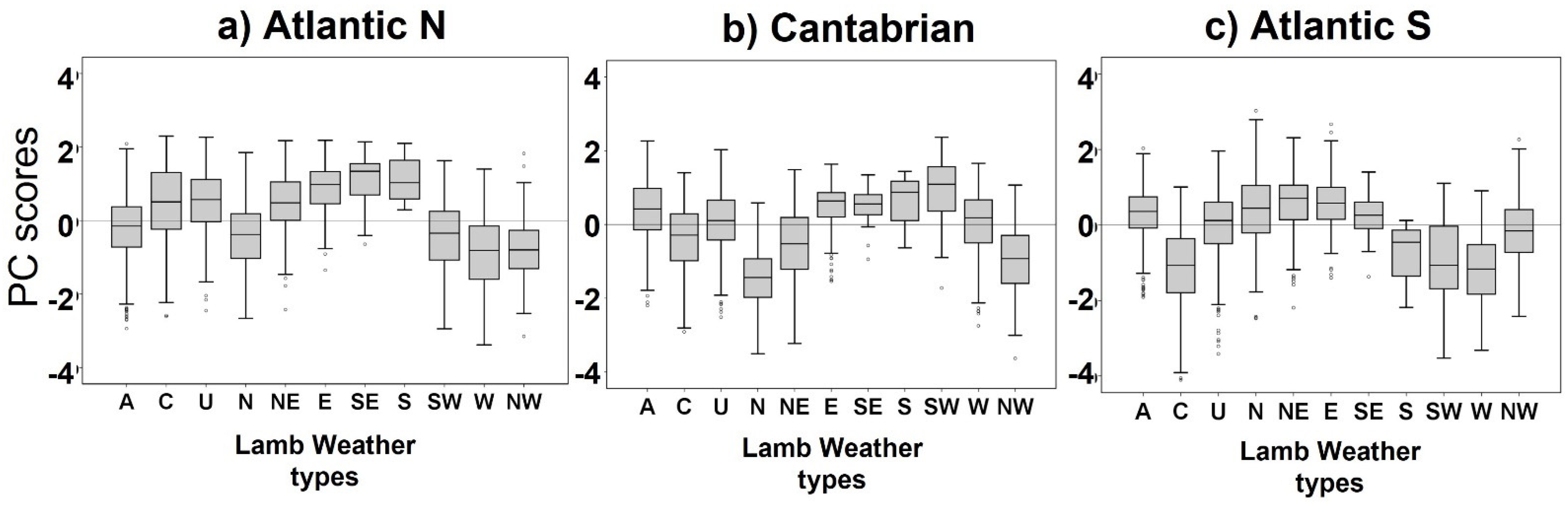
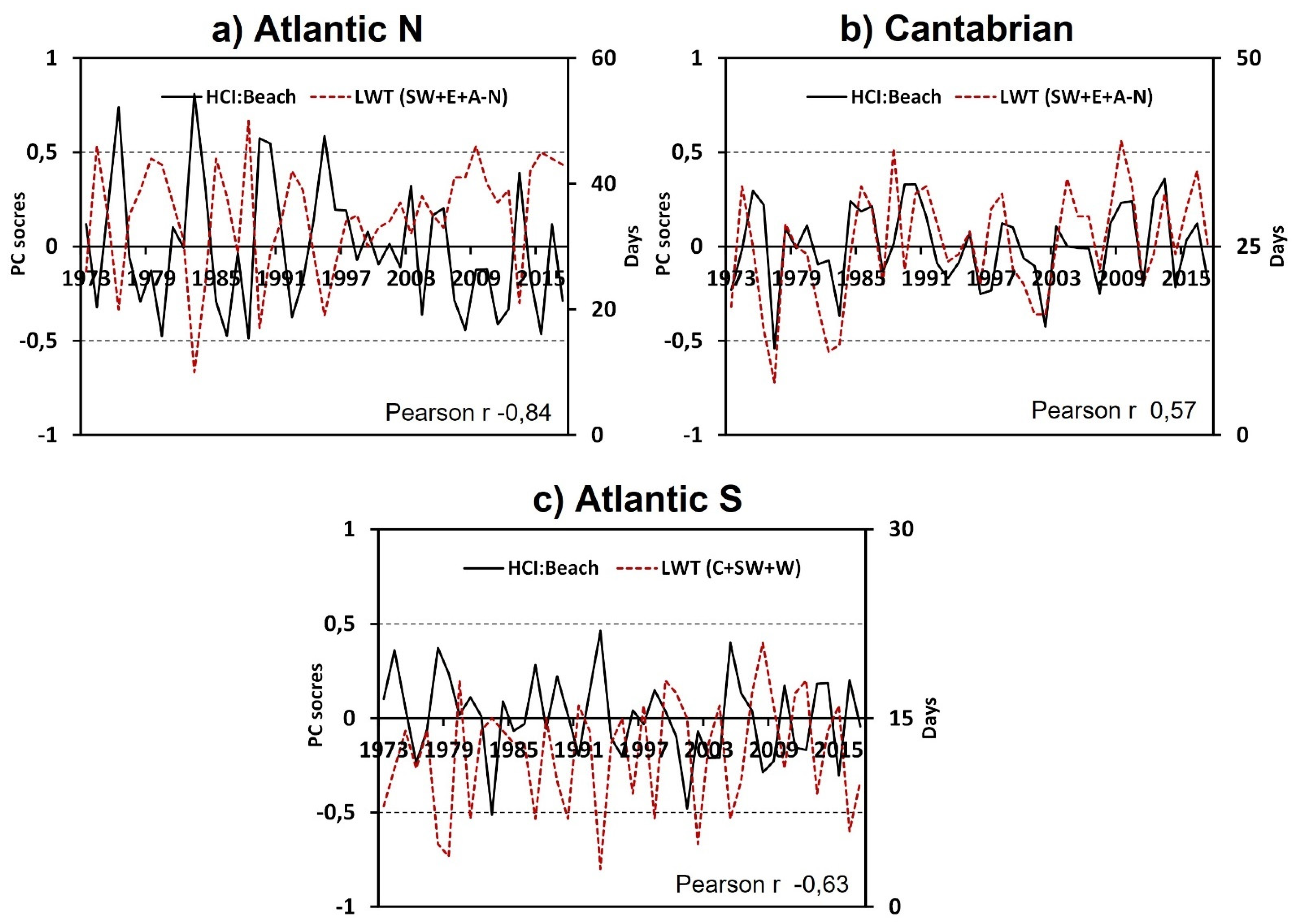
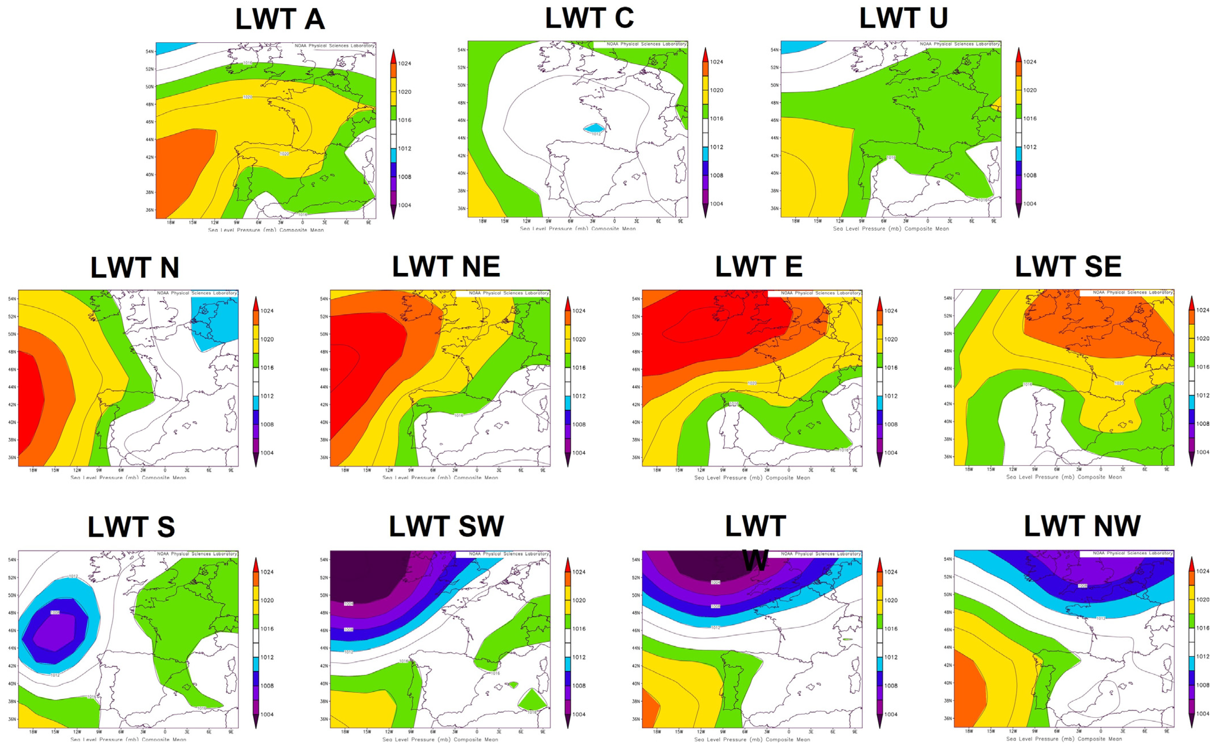
When comparing regional HCI: Beach values with the variability of LWT, a better predictive capacity has been found for the northernmost region. The proximity to the main summer Atlantic storm track means that, even in summertime, daily weather mechanisms are those typical of the mid-latitude systems. Extratropical cyclones, accompanied by frontal systems provide clouds, winds and rain (SW, W, NW, and N LWTs), while anticyclones (types E, SE and A types) cause fair weather. Indeed, convection exists within the frontal structures but is limited in time and space by the movement of the fronts. Southward, the 45° N parallel becomes a transition zone between the temperate and subtropical (Mediterranean climates). In this region, LWTs can explain a great portion of the variability of the HCI index since the most significative are also related to extratropical cyclones. However, only a few disturbances reach the area in summer, due to the greater distance to the main storm track. Consequently, the predictive capability of the LWTs diminishes in comparison with the UK and Northern France. Finally, the lowest predictive capability of LWTs is found along the northern Coast of Spain. The closest related patterns to HCI: Beach are a mixture of stable (e.g., S, SW, E and A) and unstable (N). It has been mentioned that, even during stable conditions, any northerly flow can develop a stratocumuli layer when reaching the mountains, which considerably reduces the values of the index at the coast. Additionally, the intensity of the precipitation can be substantially diverse, depending on the convective mechanisms triggered by the combination of a moist and warm surface layer (moisture transference from the warm sea water pool) and an upper cool air mass.
Summarizing, in UK and France most of the variability can be explained by regional and hemispheric processes, while in Portugal, Spain and southern France there is a larger dependence on local processes, which are more difficult to account at the scale and diagnostic tools used in this paper.
The absence of clear trends in the summer HCI: Beach index seem surprising in the context of the ongoing global warming. However, the most recent IPCC report confirms that the global warming trends are spatially, seasonally and daylight dependent [52]. Indeed, a great number of stations show trends towards high maximum temperatures, but the only coherent regional signal showing a significant warming is the Northern coast of the Iberian Peninsula. Although a more in-depth analysis of the origin of this trend is needed, it should be noted that southerly flows, identified as weather types prone to excellent HCI: Beach ratings, not only direct warm air masses over the Iberian Peninsula, but also add an additional warming when descending along the northern slope of the Cantabrian Mountains and Pyrenees, because of the thermodynamic transformations associated with the Föhn effect. However, this warming trend is balanced by the lack of any significant trend in cloudiness and precipitation, which are the variables that load the most in HCI: Beach.
In the rest of the regions, a coherent significant warming signal is not so clear, and most trends are weaker and, occasionally, non-significant. This may respond, in the first instance, to the coastal location of the stations, where the influence of the sea might weaken the trends observed in mainland stations (the weakest appear on stations placed on islands). The most stable and sunny situations, conductive to high HCI: Beach values, often generate sea breeze regimes, triggered by the thermal contrast between marine and continental surfaces. Those sea breezes direct cool and moist air masses to a narrow coastal strip, submitted to a slight cooling with respect to the mainland areas. Furthermore, it is not unknown that, if a very warm advection develops, the atmospheric layers directly in contact with the coastal waters become saturated; the increase in water vapor may create advection fogs, also affecting the weather conditions of the coastal strip [53,54]. Additionally, that thermal comfort (whose input is the HUMIDEX index) only represents one third of the total weight upon HCI: Beach, while cloudiness represents 40% and precipitation another 30%. Recent trends on climate beach-based tourism aptitude have been analyzed for different world locations and with different indices. Those results empirically support the assertion that climate change is unequally impacting the re-distribution of climate resources dependent on climate region and specific geographical characteristics. For example, the mid-latitude region of USA experienced the largest improvement from 1981 to 2019, while just a moderate improvement or even a decline was observed in the tropical and arid climate regions [39]. A significant lengthening of the annual average tourist climate comfortable period in mainland China was also found for the 1981–2010 period [40]. On the other side, trends of TCI scores did not indicate a significant change for the majority of South Africa [41], as well as in the Canary Islands [42], without any significant trend to worsening due to increased temperatures in both subtropical destinations.
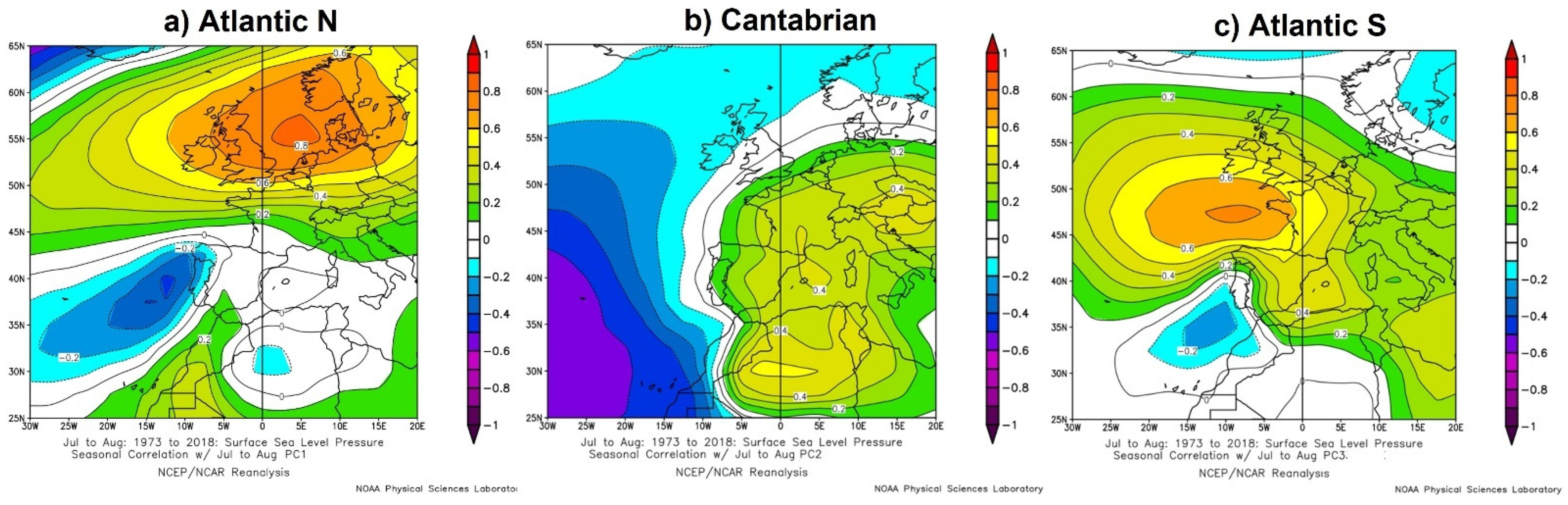
The close connection between the interannual variability of both variables in the Atlantic N region with the phase and intensity of the summer NAO [55,56] has favored the occurrence of mild, cloudy, and wet summers, particularly from 2000 onwards [57]. As with its winter counterpart, the summer NAO has shown positive (e.g., 2013, 2006, 1995, 1983, 1976 and 1975) and negative phases (e.g., 2007, 2008, 2009, 2011, 2012 and 2015). Positive phases correspond to warm, dry, and sunny summers, while negative phases tend to be associated with cool and wet summers. For example, UK summers have been on average 11% wetter than 1981–2010 and 13% wetter than 1961–1990 during the decade 2009–2018 [58].

5. Conclusions

The climate beach-based tourism aptitude of the Atlantic coasts of Western Europe and its evolution between 1973 and 2017 have been evaluated, highlighting links with atmospheric circulation. The daily value of the HCI: Beach index of 26 stations located between the Dover Strait/Pas de Calais and the N coast of Portugal was calculated and compared with a circulation pattern catalogue and indices of well-known Euro-Atlantic teleconnections. The results show a progressive decrease of the climate aptitude from S to N, organized into three homogeneous regions. Each region displays specific characteristics and temporal evolution, largely determined by the connection between geographic and atmospheric factors. During the study period, no significant temporal trend was detected in any of these areas, rather a notable interannual variability, more pronounced in the northernmost region. This same region shows the greatest links with specific circulation patterns, closely linked to the summer atmospheric circulation over the Eastern Atlantic represented by the North Atlantic Oscillation.

Funding

This research received no external funding.

Institutional Review Board Statement

Not applicable.

Informed Consent Statement

Not applicable.

Data Availability Statement

Data set available on request to corresponding authors.

Conflicts of Interest

The author declares no conflict of interest.

Appendix A

Table A1. Location of the meteorological stations. CODE stands for WMO code; CO stands for Country; LAT, LON and ALT stand for latitude, longitude (in degrees) and altitude (a.s.l); HCI stands for summer (JA) HCI: Beach average value; % ED stands for average ratio of days categorized as excellent (HCI: Beach > 80).
CODESTATIONCOLATLONALTHCI% ED
37970MANSTONUK51.3501.3335069.1223.89
38270PLYMOUTH MOUNT BATTUK50.350−4.1175065.0519.44
38620BOURNEMOUTH/HURNUK50.783−1.8331070.1927.87
38940GUERNSEY AIRPORTUK49.433−2.60010166.9821.14
70020BOULOGNEFR50.7331.6007465.5421.28
70100DUNKERQUEFR51.0502.3331766.4122.72
70280CAP DE LA HEVEFR49.5000.06710367.7126.73
70400DIEPPEFR49.9331.1003866.3822.34
71000OUESSANTFR48.483−5.0506863.7914.04
71100BRESTFR48.450−4.4179965.1820.69
72000PTE DE PENMARCHFR47.800−4.3671969.7827.92
72010QUIMPERFR47.967−4.1679467.3526.77
72050LORIENT/LAN BIHOUEFR47.767−3.4504271.2634.44
72070BELLE IIE LE TALUTFR47.300−3.1674372.2835.26
72170SAINT NAZAIRE/MONTOFR47.317−2.167374.4343.41
73000L IIE D YEUFR46.700−2.3333274.7743.04
73140CHASSIRONFR46.050−1.4172276.5648.97
75020CAZAUXFR44.533−1.1332475.2846.19
76020BIARRITZFR43.467−1.5337171.5137.89
80010LA CORUNASP43.367−8.4176776.8850.21
80110ASTURIAS/AVILESSP43.550−6.03313073.1136.62
80210SANTANDER/PARAYASSP43.433−3.817973.5441.97
80250BILBAO/SONDICASP43.300−2.9003972.6138.40
80290SAN SEBASTIAN/FUENTSP43.350−1.800871.3738.16
80450VIGO/PEINADORSP42.233−8.63325579.363.01
85450PORTO/PEDRAS RUBRASPO41.233−8.6837782.2268.52

Appendix B

As mentioned in the paper, the HCI: Beach uses five weather variables (temperature, humidity, cloud cover, precipitation, and wind speed) to derive three sub-indices accounting for the thermal, aesthetic, and physical dimensions of climate relevant to tourism.
Each component owes a different weight on the final formula (Table 1), which is:
HCI: Beach = 2(TC) + 4(A) + 3(P) + W
Table A2. Weather components and weighting.
Index ComponentVariableHCI Weights
Thermal comfort (TC)Humidex Temperature (°C)20%
Aesthetic (A)Cloud cover (%)40%
PhysicalTotal precipitation (mm)30%
PhysicalMean wind speed (km/h)10%
Each of the sub-indices in the HCI:Beach can score up to 10 (Table 2, Table 3 and Table 4), adding up to an overall climate rating that ranges from 0 (impossible/dangerous) to 100 (ideal). The rating scores correspond with descriptive categories that change at 10-point increments (e.g., 50–59 points is “acceptable”, 60–69 is “good”, 70–79 is very good, 80–89 is excellent, 90+ is ideal).
Instead of just temperature, thermal comfort combines temperature and relative humidity for the thermal comfort component of the index. The Canadian Humidex (or humidity index) is used to quantify the thermal well-being of the bathers. The formulae to calculate humidex is the following.
Humidex = T a i r + 0.5555 [ 6.11 e 5417.7530 ( 1 273.16 + 1 273.15 + T d e w ) 10 ]
Although the index is nominally a dimensionless quantity, public perception has considered the values as equivalent to degree Celsius.
Table A3. Thermal comfort facet rating values.
Humidex (°C)Rating
≥390
38 to 38.92
37 to 37.94
36 to 36.95
35 to 35.96
34 to 34.97
33 to 33.98
31 to 32.99
28 to 30.910
26 to 27.99
23 to 25.97
22 to 22.96
21 to 21.95
20 to 20.94
19 to 19.93
18 to 18.92
17 to 17.91
15 to 16.90
10 to 14.9−5
≤9.9 to−10
Table A4. Aesthetic facet rating values.
Cloud Cover (%)Rating
0–0.98
1–14.99
15–25.910
26–35.99
36–45.98
46–55.97
56–65.96
66–75.95
76–85.94
86–95.93
≥962
Table A5. Physical facet rating values (precipitation).
Precipitation (mm)Rating
010
0.01–2.999
3.0–5.998
6.0–8.996
9.0–11.994
12.0–24.990
≥25−1
Table A6. Physical facet rating values (wind speed).
Wind Speed (km/h)Rating
0–0.58
0.6–9.910
10.0–19.99
20.0–29.98
30.0–39.96
40.0–49.93
50.0–69.90
≥70−10

Appendix C

Lamb Weather Types (LWTs)
Based on Jenkinson and Collison (1977) procedures developed to define objectively LWTs for the British Isles, circulation patterns are obtained from a set of indices associated to the direction and vorticity of geostrophic flow, derived from sea level pressure data (Figure 1).
Figure A1. Grid points used to compute the flow indices.
Atmosphere 12 01328 g0a1
The indices used were the following:
  • W: The zonal component of geostrophic (surface) wind, calculated as the pressure gradient between 45° N and 65° N
  • S: The meridional component of geostrophic (surface) wind, calculated as the pressure gradient between 40° W and 70° W
  • D: The wind direction (azimuth degree) derived from S and W above
  • F: The wind speed (ms−1)
  • ZW: The zonal vorticity component
  • ZS: The meridional vorticity component
  • Z: The total vorticity derived from ZW and ZS.
The indices are calculated from the following set of equations, where the SLP integers’ subscripts correspond to the grid point reference numbers in Figure 1:
W = 1 2 ( S L P 12 + S L P 13 ) 1 2 ( S L P 4 + S L P 5 )
S = 1.74 [ 1 4 ( S L P 5 + 2   S L P 9 + S L P 13 ) 1 4 ( S L P 4 + 2   S L P 8 + S L P 12 ) ]
F = ( S 2 + W 2 ) 1 / 2
Z W = 1.1 [ 1 2 ( S L P 15 + S L P 16 ) 1 2 ( S L P 8 + S L P 9 ) ] 0.95 [   1 2 ( S L P 8 + S L P 9 ) 1 2 ( S L P 1 + S L P 2 ) ]
Z S = 1.0 [ 1 4 ( S L P 6 + 2   S L P 10 + S L P 14 ) 1 4 ( S L P 5 + 2   S L P 9 + S L P 13 ) 1 4 ( S L P 4 + 2   S L P 8 + S L P 12 ) 1 4 ( S L P 3 + 2   S L P 7 + S L P 11 ) ]
Z = Z W + Z S
The following set of rules allow to define different types of circulation:
  • Direction of flow is given by tan−1 (WF/SF), 180° being added if WF is positive. The appropriate direction is computed using an eight-point compass, allowing 45° per sector.
  • If |Z| < F, flow is essentially straight and considered to be of a pure directional type (eight different cases according to the compass directions).
  • If |Z| > 2 F, the pattern is considered to be of a pure cyclonic type if Z > 0, or of a pure anticyclonic type if |Z| < 0.
Composite maps of each CWT were computed for the summer months (JA) of the period 1973–2017. Figure 2 displays a composite example of each CWT.
Figure A2. SLP fields characteristic of the ten basic summer (JA) CWTs. The contour interval is 2 hPa. Images provided by the NOAA/ESRL Physical Sciences Laboratory, Boulder Colorado from their Web site at http://psl.noaa.gov/ (accessed on 31 August 2021).
Atmosphere 12 01328 g0a2

References

  1. Tadaki, M.; Salmond, J.; Le Heron, R. Applied climatology. Prog. Phys. Geog. 2014, 38, 392–413. [Google Scholar] [CrossRef]
  2. Scott, D.J.; Lemieux, C.J.; Malone, L. Climate services to support sustainable tourism and adaptation to climate change. Clim. Res. 2011, 47, 111–122. [Google Scholar] [CrossRef] [Green Version]
  3. Rosselló, J.; Waqas, A. The use of tourism demand models in the estimation of the impact of climate change on tourism. Turismo em Análise 2015, 26, 4–20. [Google Scholar] [CrossRef] [Green Version]
  4. Smith, K. The influence of weather and climate on recreation and tourism. Weather 1993, 48, 398–404. [Google Scholar] [CrossRef]
  5. Roux, S.; Giet, E. Tourist characteristics in France. J. App. Sci. Trav. Hosp. 2019, 2, 78–84. [Google Scholar] [CrossRef]
  6. Besancenot, J.P.; Mounier, J.; de Lavenne, F. Les conditions climatiques du tourisme littoral. Norois 1978, 99, 357–382. [Google Scholar] [CrossRef]
  7. Besancenot, J.P. Climat et tourisme estival sur les côtes de la péninsule ibérique. Revue Géographique des Pyrénées et du Sud-Ouest 1985, 4, 427–449. [Google Scholar] [CrossRef]
  8. Moreno, A.; Amelung, B.; Santamarta, L. Linking beach recreation to weather conditions: A case study in Zandvoort, Netherlands. Tour. Mar. Environ. 2008, 5, 111–119. [Google Scholar] [CrossRef]
  9. Gómez-Martín, M.B.; Martinez-Ibarra, E. Tourism demand and atmospheric parameters: Non-intrusive observation techniques. Clim. Res. 2012, 51, 135–145. [Google Scholar] [CrossRef] [Green Version]
  10. Toubes, D.; Araújo-Vila, N.; Fraiz-Brea, J.A. Influence of weather on the behaviour of tourists in a beach destination. Atmosphere 2020, 11, 121. [Google Scholar] [CrossRef] [Green Version]
  11. ICANE. Perfil del turista en Cantabria Año 2018. Instituto Cántabro de Estadística. Consejería de Economía y Hacienda, Gobierno de Cantabria. 2018. Available online: https://www.icane.es/c/document_library/get_file?uuid=f73d32ba-4d90-43ad-ad61-d5db667b17e7&groupId=10138#:~:text=Perfil%20del%20turista%20en%20Cantabria%20A%C3%B1o%202018%20Demanda,4%2C02%203%2C2%20Asturias%20%28Principado%20de%29%204.961.049%202%2C51%203%2C5 (accessed on 27 September 2021).
  12. Zielinski, S.; Botero, C. Beach tourism in times of COVID-19 pandemic: Critical Issues, knowledge gaps and research opportunities. Int. J. Environ. Res. Public Health 2020, 17, 7288. [Google Scholar] [CrossRef] [PubMed]
  13. Gössling, S.; Scott, D.; Hall, C.M. Pandemics, tourism and global change: A rapid assessment of COVID-19. J. Sustain. Tour. 2020, 29, 1–20. [Google Scholar] [CrossRef]
  14. Grillakis, M.; Koutroulis, A.; Seiradakis, K.; Tsanis, I. Implications of 2 °C global warming in European summer tourism. Clim. Serv. 2016, 1, 30–38. [Google Scholar] [CrossRef] [Green Version]
  15. Koutroulis, A.; Grillakis, M.; Tsanis, I.; Jacob, D. Mapping the vulnerability of European summer tourism under 2 °C global warming. Clim. Chang. 2018, 151, 157–171. [Google Scholar] [CrossRef]
  16. Amengual, A.; Homar, V.; Romero, R.; Ramis, C.; Alonso, S. Projections for the 21st century of the climate potential for beach-based tourism in the Mediterranean. Int. J. Climatol. 2014, 34, 3481–3498. [Google Scholar] [CrossRef] [Green Version]
  17. Hamilton, J.M.; Maddison, D.J.; Tol, R.S.J. Climate change and international tourism: A simulation study. Glob. Environ. Chang. 2005, 15, 253–266. [Google Scholar] [CrossRef]
  18. Amelung, B.; Viner, D. Mediterranean tourism: Exploring the future with the tourism climatic index. J. Sustain. Tour. 2006, 14, 349–366. [Google Scholar] [CrossRef]
  19. Hein, L.; Metzger, M.J.; Moreno, A. Potential impacts of climate change on tourism; a case study for Spain. Curr. Opin. Environ. Sustain. 2009, 1, 170–178. [Google Scholar] [CrossRef]
  20. Rutty, M.; Scott, D. Will the Mediterranean become “too hot” for tourism? A reassessment. Tour. Hosp. Plan. Dev. 2010, 7, 267–281. [Google Scholar] [CrossRef]
  21. Bujosa, A.; Rosselló, J. Climate change and summer mass tourism: The case of Spanish domestic tourism. Clim. Chang. 2012, 117, 363–375. [Google Scholar] [CrossRef]
  22. Amelung, B.; Nicholls, S.; Viner, D. Implications of global climate change for tourism flows and seasonality. J. Travel Res. 2007, 45, 285–296. [Google Scholar] [CrossRef]
  23. Mieczkowski, Z. The tourism climate index: A method for evaluating world climate for tourism. Can. Geogr. 1985, 29, 220–233. [Google Scholar] [CrossRef]
  24. Morgan, R.; Gatell, E.; Junyent, R.; Micallef, A.; Özhan, E.; Williams, A.T. An improved user-based beach climate index. J. Coast Conserv. 2000, 6, 41–50. [Google Scholar] [CrossRef] [Green Version]
  25. Yu, G.; Schwartz, Z.; Walsh, J.E. A weather resolved index for assessing the impact of climate change on tourism related climate resources. Clim. Chang. 2009, 95, 551–573. [Google Scholar] [CrossRef]
  26. Scott, D.; Rutty, M.; Amelung, B.; Tang, M. An inter-comparison of the holiday climate index (HCI) and the tourism climate index (TCI) in Europe. Atmosphere 2016, 7, 80. [Google Scholar] [CrossRef] [Green Version]
  27. Rutty, M.; Scott, D.; Matthews, L.; Burrowes, R.; Trotman, A.; Mahon, R.; Charles, A. An inter-comparison of the holiday climate index (HCI: Beach) and the tourism climate index (TCI) to explain Canadian tourism arrivals to the Caribbean. Atmosphere 2020, 11, 412. [Google Scholar] [CrossRef] [Green Version]
  28. De Freitas, C. Tourism climatology: Evaluating environmental information for decision making and business planning in the recreation and tourism sector. Int. J. Biometeorol. 2003, 48, 45–54. [Google Scholar] [CrossRef] [PubMed]
  29. Scott, D.; Gössling, S.; De Freitas, C.R. Preferred climates for tourism: Case studies from Canada, New Zealand and Sweden. Clim. Res. 2008, 38, 61–73. [Google Scholar] [CrossRef] [Green Version]
  30. Moreno, A. Mediterranean tourism and climate (change): A survey-based study. Tour. Hosp. Plan Dev. 2010, 7, 253–265. [Google Scholar] [CrossRef]
  31. Ibarra, E.M. The use of webcam images to determine tourist–climate aptitude: Favorable weather types for sun and beach tourism on the Alicante coast (Spain). Int. J. Biometeorol. 2011, 55, 373–385. [Google Scholar] [CrossRef]
  32. Rutty, M.; Scott, D. Bioclimatic comfort and the thermal perceptions and preferences of beach tourists. Int. J. Biometeorol. 2015, 59, 37–45. [Google Scholar] [CrossRef] [PubMed]
  33. Georgopoulou, E.; Mirasgedis, S.; Sarafidis, Y.; Hontou, V.; Gaki, N.; Lalas, D.P. Climatic preferences for beach tourism: An empirical study on Greek islands. Theor. Appl. Climatol. 2019, 137, 667–691. [Google Scholar] [CrossRef]
  34. Yu, D.; Rutty, M.; Scott, D.; Li, S. A comparison of the holiday climate index: Beach and the tourism climate index across coastal destinations in China. Int. J. Biometeorol. 2020, 65, 741–748. [Google Scholar] [CrossRef]
  35. Matthews, L.; Scott, D.; Andrey, J. Development of a data-driven weather index for beach parks tourism. Int. J. Biometeorol. 2021, 65, 749–762. [Google Scholar] [CrossRef]
  36. Demiroglu, O.C.; Saygili-Araci, F.S.; Pacal, A.; Hall, C.M.; Kurnaz, L.M. Future holiday climate index (HCI) performance of urban and beach destinations in the Mediterranean. Atmosphere 2020, 11, 911. [Google Scholar] [CrossRef]
  37. Rozbicka, K.; Rozbicki, T. Long-term variability of bioclimatic conditions and tourism potential for Warsaw agglomeration (Poland). Int. J. Biometeorol. 2021, 65, 1485–1495. [Google Scholar] [CrossRef]
  38. Bartzokas, A.; Lolis, C.J.; Kassomenos, P.A.; McGregor, G.R. Climatic characteristics of summer human thermal discomfort in Athens and its connection to atmospheric circulation. Nat. Hazards Earth Syst. Sci. 2013, 13, 3271–3279. [Google Scholar] [CrossRef] [Green Version]
  39. Ma, S.; Craig, C.; Feng, S.; Liu, C. Climate resources at United States National Parks: A tourism climate index approach. Tour. Recreat. Res. 2021, 1–15. [Google Scholar] [CrossRef]
  40. Yu, D.D.; Li, S.; Guo, Z. Evaluating the tourist climate comfortable period of China in a changing climate. Adv. Meteorol. 2020, 2020, 8886316. [Google Scholar] [CrossRef]
  41. Fitchett, J.M.; Robinson, D.; Hoogendoorn, G. Climate suitability for tourism in South Africa. J. Sustain. Tour. 2017, 25, 851–867. [Google Scholar] [CrossRef]
  42. Alonso-Pérez, S.; López-Solano, J.; Rodríguez-Mayor, L.; Márquez-Martinón, J.M. Evaluation of the tourism climate index in the Canary Islands. Sustainability 2021, 13, 7042. [Google Scholar] [CrossRef]
  43. Met Office. Met Office Integrated Data Archive System (MIDAS) Land and Marine Surface Stations Data (1853-current). NCAS British Atmospheric Data Centre. 2021. Available online: http://catalogue.ceda.ac.uk/uuid/220a65615218d5c9cc9e4785a3234bd0 (accessed on 27 September 2021).
  44. Smith, A.; Lott, N.; Vose, R. The integrated surface database: Recent developments and partnerships. Bull. Am. Met. Soc. 2011, 92, 704–708. [Google Scholar] [CrossRef]
  45. Pohlert, T. Package Trend. Non-Parametric Trend Tests and Change-Point Detection. R package version 1.1.14. Available online: https://cran.r-project.org/web/packages/trend/trend.pdf (accessed on 31 August 2021).
  46. Kalnay, E.; Kanamitsu, M.; Kistler, R.; Collins, W.; Deaven, D.; Gandin, L.; Iredell, M.; Saha, S.; White, G.; Woollen, J.; et al. The NMC/NCAR 40-year reanalysis project. Bull. Am. Meteorol. Soc. 1996, 77, 437–471. [Google Scholar] [CrossRef] [Green Version]
  47. Preisendorfer, R.W.; Mobley, C.D. Principal Component Analysis in Meteorology and Oceanography; Elsevier: Amsterdam, The Netherlands, 1988. [Google Scholar]
  48. Wilks, D.S. Statistical Methods in the Atmospheric Sciences; Academic Press: Cambridge, MA, USA, 2011. [Google Scholar]
  49. Yarnal, B. Synoptic Climatology in Environmental Analysis: A Primer; Belhaven Press: London, UK, 1993. [Google Scholar]
  50. Jenkinson, A.F.; Collison, F.P. An Initial Climatology of Gales over the North Synoptic Climatology; Branch Memorandum NO.62; UK Met Office: Bracknell, UK, 1977.
  51. Uriarte Cantolla, A. Régimen de Precipitaciones en la Costa NW y N de la Península Ibérica. Doctoral Thesis, Universidad de Zaragoza, Saragossa, Spain, 1980. (In Spanish). [Google Scholar]
  52. IPCC. Summary for POLICYMAKERS. In Climate Change 2021: The Physical Science Basis; Contribution of Working Group I to the Sixth Assessment Report of the Intergovernmental Panel on Climate Change; Masson-Delmotte, V.P., Zhai, A., Pirani, S.L., Connors, C., Péan, S., Berger, N., Caud, Y., Chen, L., Goldfarb, M.I., Gomis, M., et al., Eds.; Cambridge University Press: Cambridge, UK, 2021. [Google Scholar]
  53. Planchon, O. A study of the coastal climates in France using temperature and precipitation data (1961–1990). Meteorol. Appl. 2000, 7, 217–228. [Google Scholar] [CrossRef]
  54. Bigot, S.; Planchon, O. Identification and characterization of sea breeze days in Northern France using singular value decomposition. Int. J. Climatol. 2000, 23, 1397–1405. [Google Scholar] [CrossRef]
  55. Bladé, I.; Liebmann, B.; Fortun, D.; van Oldenborgh, G.J. Observed and simulated impacts of the summer NAO in Europe: Implications for projected drying in the Mediterranean region. Clim. Dyn. 2012, 39, 709–727. [Google Scholar] [CrossRef]
  56. Dong, B.; Sutton, R.T.; Woollings, T.; Hodges, K. Variability of the North Atlantic summer storm track: Mechanisms and impacts on the European climate. Environ. Res. Lett. 2013, 8, 034037. [Google Scholar] [CrossRef]
  57. Hanna, E.; Cropper, T.E.; Jones, P.D.; Scaife, A.A.; Allan, R. Recent seasonal asymmetric changes in the NAO (a marked summer decline and increased winter variability) and associated changes in the AO and Greenland Blocking Index. Int. J. Climatol. 2015, 35, 2540–2554. [Google Scholar] [CrossRef]
  58. Kendon, M.; McCarthy, M.; Jevrejeva, S.; Matthews, A.; Legg, T. State of the UK climate 2018. Int. J. Climatol. 2019, 39 (Suppl. 1), 1–55. [Google Scholar] [CrossRef] [Green Version]
Figure 1. Location of the study area. Extended information about stations identified with red numbers appear in Appendix A.
Atmosphere 12 01328 g001
Figure 2. (a) Monthly averages of the HCI: Beach index in selected locations of the study area; (b) Spatial anomalies of the summer (July–August) HCI: Beach after regression against latitude.
Atmosphere 12 01328 g002
Figure 3. Regionalization of the summer (JA) daily HCI: Beach index on the study area based on the Principal Component loadings matrix.
Atmosphere 12 01328 g003
Figure 4. Box plot showing the within-group variance of daily PC scores according to each LWT for the (a) Atlantic N region (b) Cantabrian region and (c) Atlantic S region. The boxplot presents the median, maximum, minimum, lower, and upper quartile of daily values. Outliers, represented as dots, are also indicated as any point falling below QL—1.5 × inter quartile range (IQR) or above QU—1.5 × IQR, where IQR is the difference between the two quartiles. X axis labels correspond to each LWT (see Appendix C).
Atmosphere 12 01328 g004
Figure 5. Normalized values of HCI: Beach index (thin line) and number of days corresponding to the most favorable LWT (dot line) for the (a) Atlantic N region (b) Cantabrian region (c) Atlantic S. The corresponding correlation coefficient is also presented.
Atmosphere 12 01328 g005
Figure 6. Correlation maps between times series of the Principal Component scores for the (a) Atlantic N region (b) Cantabrian Region (c) Atlantic S region and sea level pressure fields. Values higher (lower) than 0.31 (−0.31) are significant at the 95% significance level, according to a t-test. Images provided by the NOAA/ESRL Physical Sciences Laboratory, Boulder Colorado from their Web site at http://psl.noaa.gov/, accessed on m 31 August 2021).
Atmosphere 12 01328 g006
Table 1. Values of the Pearson Correlation Coefficient between latitude and original climate variables and derived variables after the calculation of HCI: Beach. ** stands for values statistically significant at the 99% confidence level.
VariablePearson Correlation Coefficient
Seasonal average value of HCI: Beach−0.81 **
Frequency of days with HCI: Beach < 600.76 **
Frequency of days with HCI: Beach > 80−0.84 **
Temperature (°C)−0.74 **
Relative Humidity (%)0.31
Humidex (°C)−0.83 **
Cloud Cover (oktas)0.66 **
Daily Precipitation (mm)0.19
Wind speed (km/h)0.78 **
Frequency of wet days (precipitation > 1 mm)−0.51 **
Table 2. Values of the statistic Z of a Mann-Kendall test and Q from a Sen’s slope corresponding to the temporal evolution between 1973 and 2017 of the component scores of each PC.
VariablesMann_Kendall ZSen’s Slope Q
Atlantic N−0.89−0.04 values/dec
Cantabrian−0.020.00 values/dec
Atlantic S−1.40−0.04 values/dec
Table 3. F-values and significance from an ANOVA procedure to determine whether the mean values of the Principal Component scores within the synoptic categories were significantly different, and selected circulation pattern on each region.
RegionF-ValueSignificationBest LWT Combination
Atlantic N130.4220.000+SW, +W, +NW, +N
Cantabrian154.5640.000+SW, +E, +A, −N
Atlantic S127.6900.000+SW, +W, +C
Table 4. Values of the Pearson Correlation coefficient between the PC scores corresponding to each region and the corresponding values of the main teleconnection patterns affecting the Atlantic and Europe. ** stands for values statistically significant at the 99% confidence level; * stands for values statistically significant at the 95% confidence level.
VariablesAtlantic NCantabrianAtlantic S
NAO (North Atlantic Oscillation)0.62 **−0.07−0.10
EA (Eastern Atlantic Oscillation)−0.32 *−0.11−0.12
EA_WR (Eastern Atlantic Western Russia Oscillation−0.040.17−0.16
SCAND (Scandinavian Oscillation)0.18−0.28−0.18
Publisher’s Note: MDPI stays neutral with regard to jurisdictional claims in published maps and institutional affiliations.

