
Modeling the Impacts of City-Scale “Ventilation Corridor” Plans on Human Exposure to Intra-Urban PM2.5 Concentrations


Abstract
:1. Introduction
2. Methods
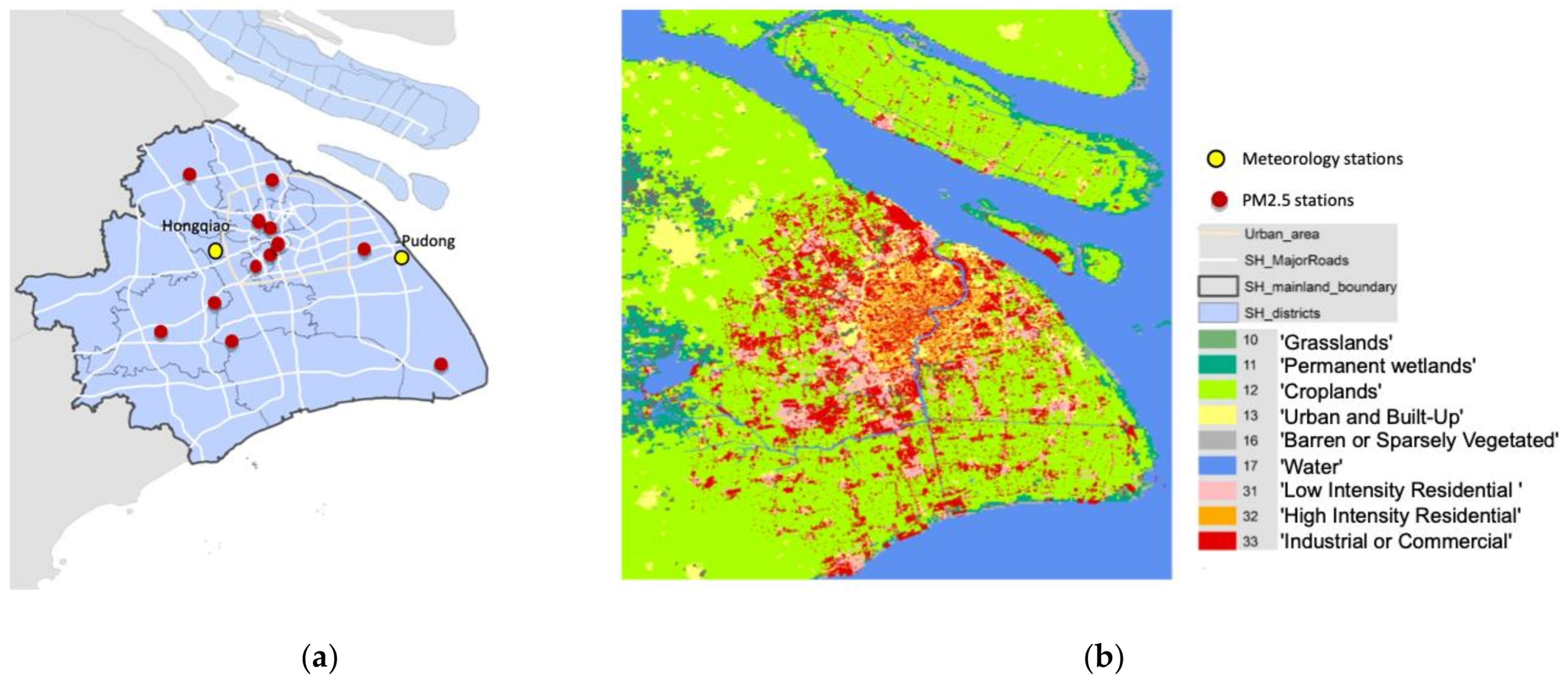
2.1. Case Study Area and Observed Data
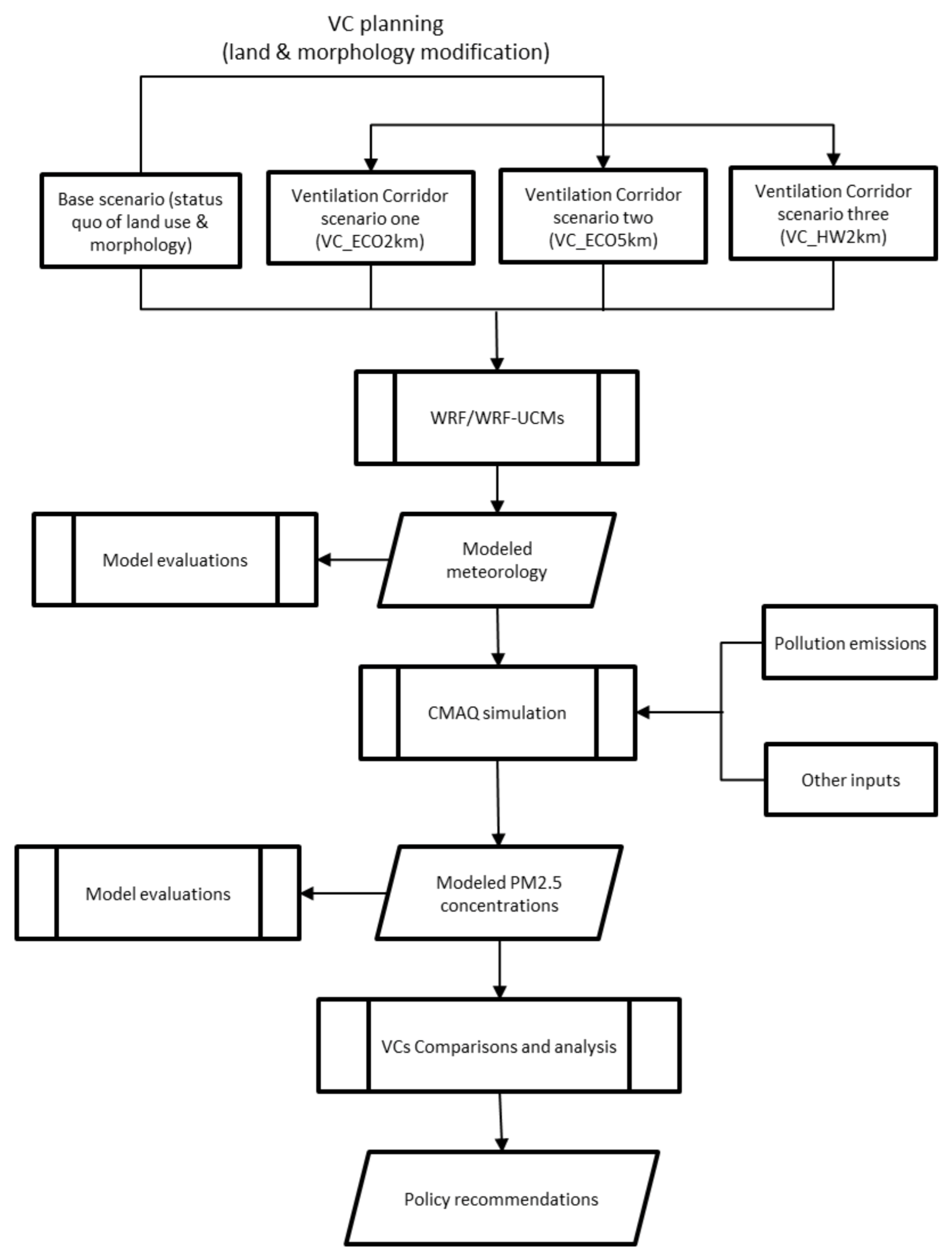
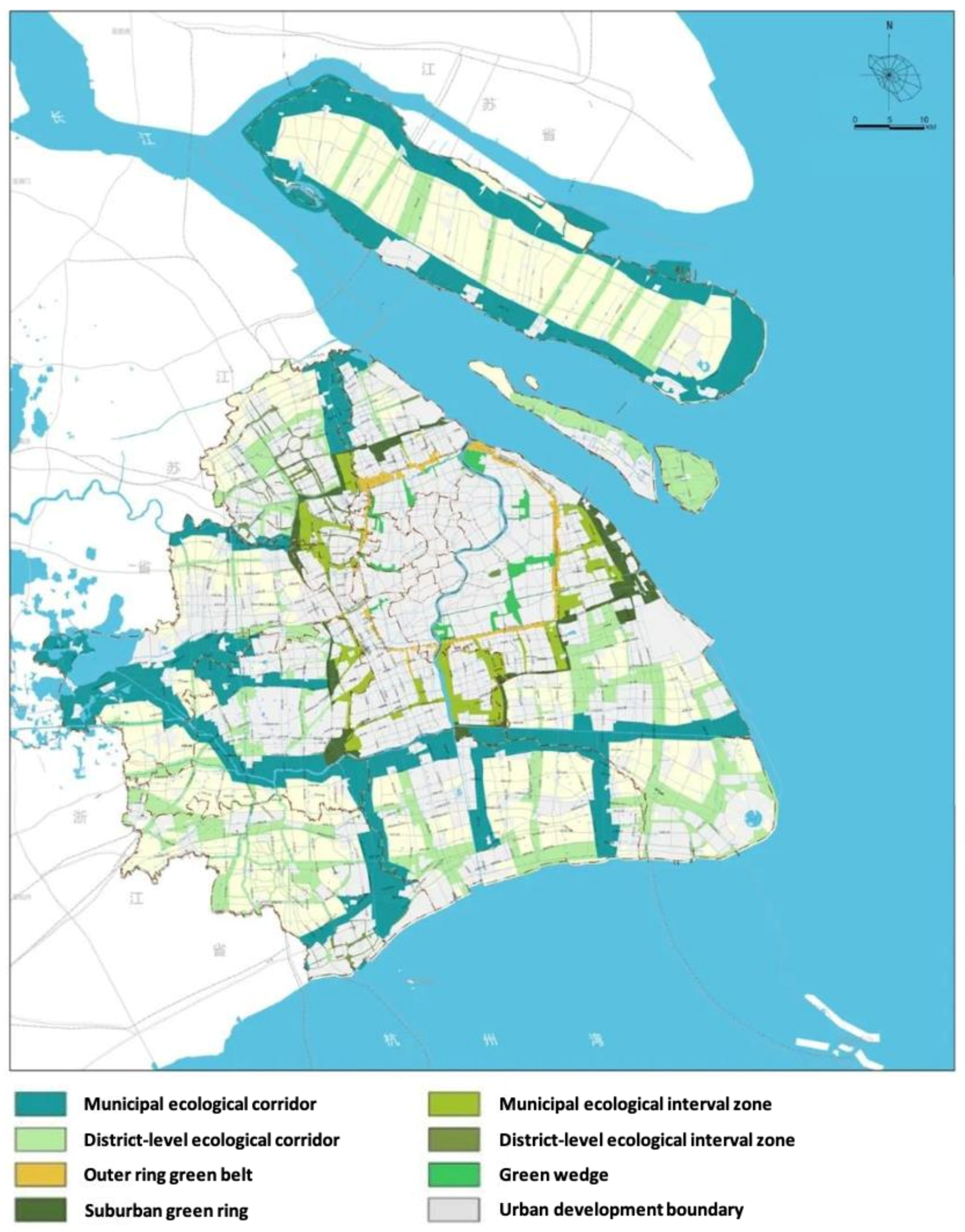
2.2. VC Planning Scenarios
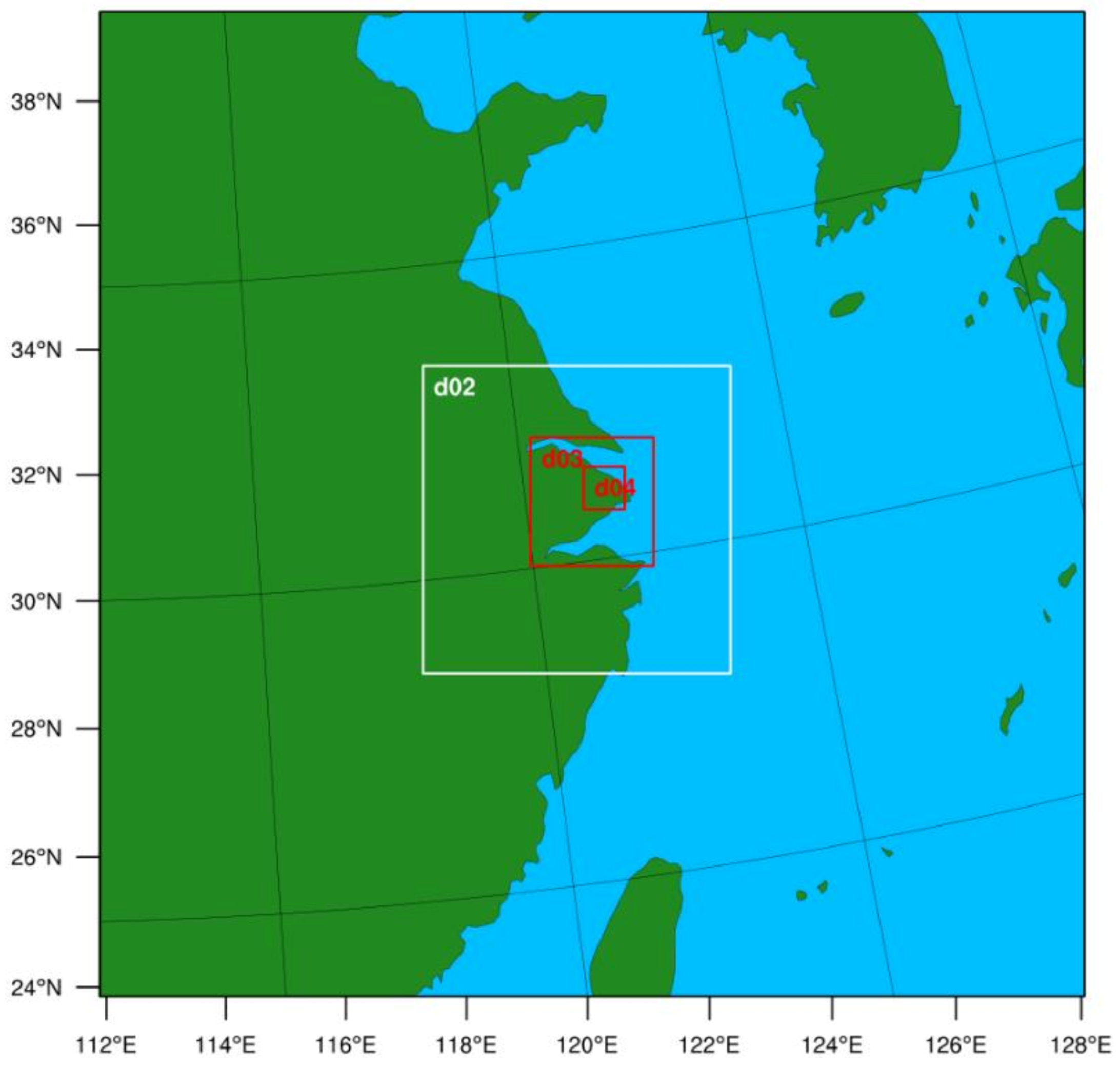
2.3. The WRF-UCM Modeling System
2.4. CMAQ Simulations of PM2.5 Pollution
2.5. Model Evaluations
2.6. Assessing VCs’ Impacts on Wind Velocity and PM2.5 Concentrations
3. Results
3.1. Evaluation Results
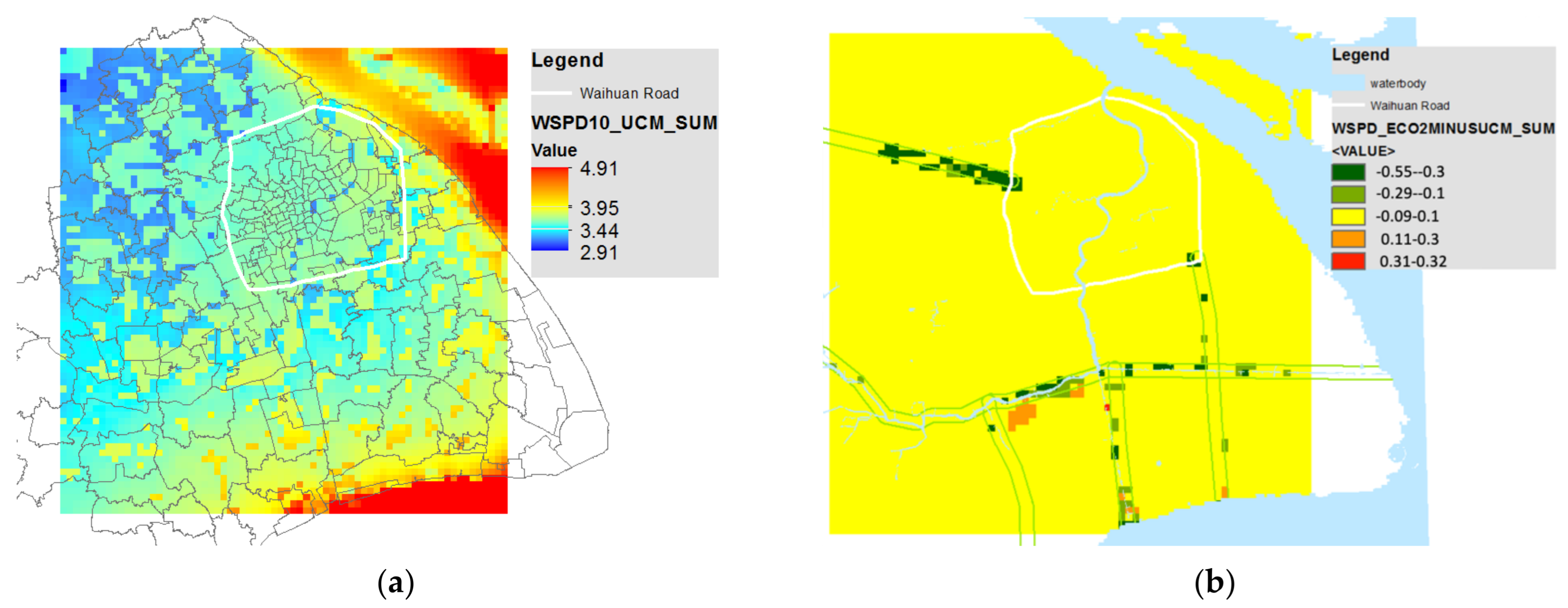
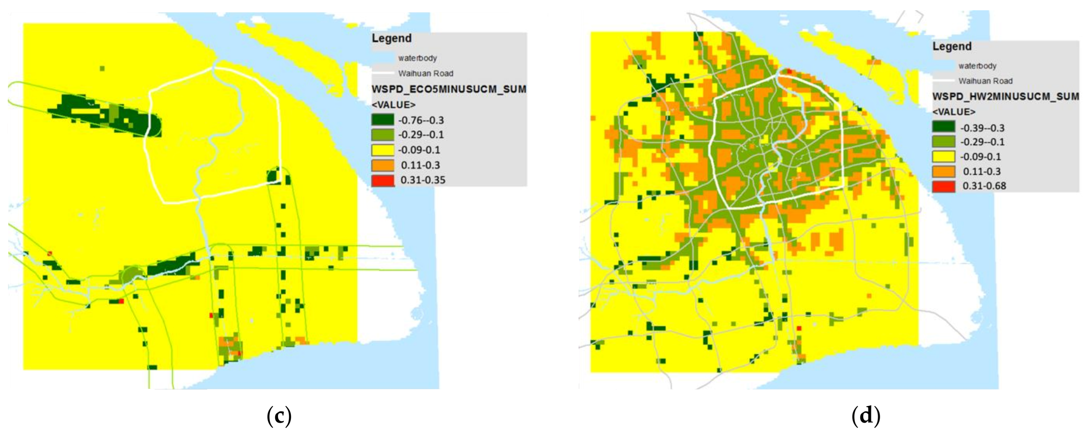
3.2. VCs Impacts on Ground Wind Velocity
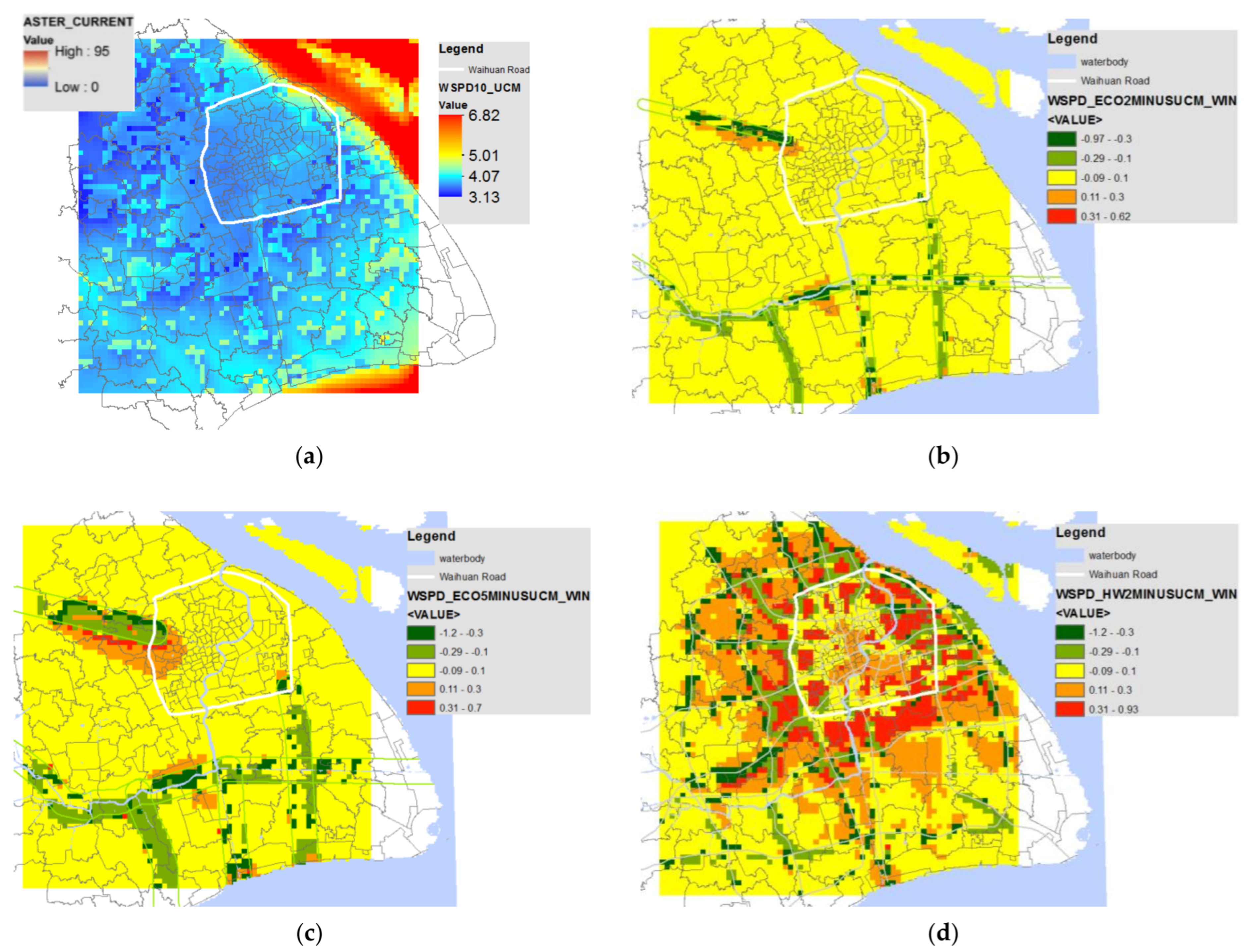
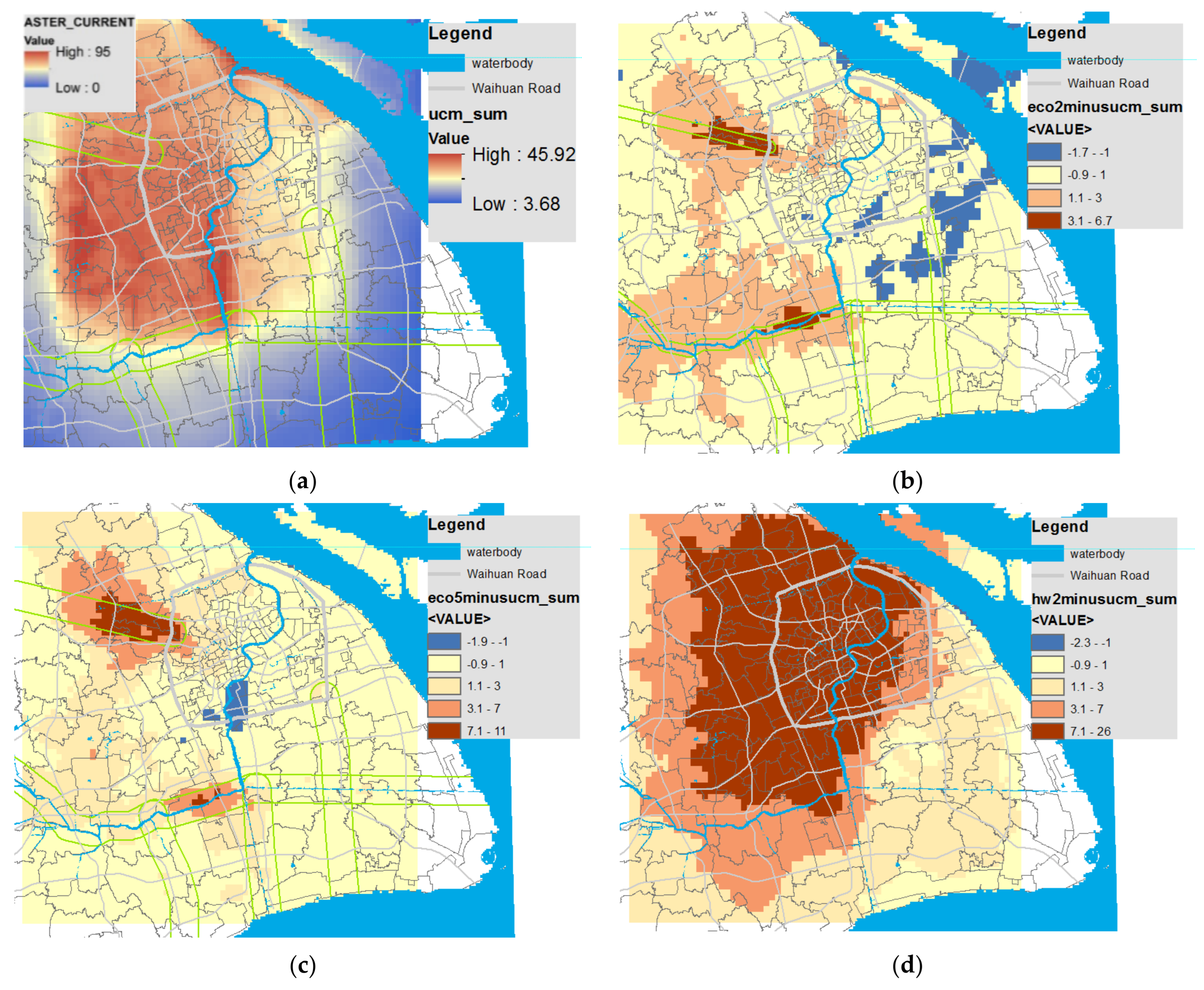
3.3. VC Impacts on PM2.5 Concentrations
4. Discussion and Links to Previous Studies
5. Conclusions
Supplementary Materials
Author Contributions
Funding
Institutional Review Board Statement
Informed Consent Statement
Acknowledgments
Conflicts of Interest
References
- Huang, L.; Rao, C.; van der Kuijp, T.J.; Bi, J.; Liu, Y. A comparison of individual exposure, perception, and acceptable levels of PM2. 5 with air pollution policy objectives in China. Environ. Res. 2017, 157, 78–86. [Google Scholar] [CrossRef] [PubMed]
- Long, Y.; Wang, J.; Wu, K.; Zhang, J. Population exposure to ambient PM2. 5 at the subdistrict level in China. Int. J. Environ. Res. Public Health 2018, 15, 2683. [Google Scholar] [CrossRef] [PubMed] [Green Version]
- Ren, C.; Yuan, C.; Ho, C.K.; NG, Y.Y. A study of air path and its application in urban planning. Urban Plan. Forum 2014, 3, 52–60. [Google Scholar]
- Kastner-Klein, P.; Plate, E. Wind-tunnel study of concentration fields in street canyons. Atmos. Environ. 1999, 33, 3973–3979. [Google Scholar] [CrossRef]
- Taseiko, O.V.; Mikhailuta, S.V.; Pitt, A.; Lezhenin, A.A.; Zakharov, Y.V. Air pollution dispersion within urban street canyons. Atmos. Environ. 2009, 43, 245–252. [Google Scholar] [CrossRef]
- Yuan, C.; Ng, E.; Norford, L.K. Improving air quality in high-density cities by understanding the relationship between air pollutant dispersion and urban morphologies. Build. Environ. 2014, 71, 245–258. [Google Scholar] [CrossRef]
- Yu, K.; Zhang, L.; Yanng, Z.; Wang, X.; Liu, M. Eco-city Construction. In Contemporary Ecology Research in China; Springer: Berlin/Heidelberg, Germany, 2015; pp. 555–624. [Google Scholar]
- Tominaga, Y.; Stathopoulos, T. CFD simulation of near-field pollutant dispersion in the urban environment: A review of current modeling techniques. Atmos. Environ. 2013, 79, 716–730. [Google Scholar] [CrossRef] [Green Version]
- Papangelis, G.; Tombrou, M.; Dandou, A.; Kontos, T. An urban “green planning” approach utilizing the Weather Research and Forecasting (WRF) modeling system. A case study of Athens, Greece. Landsc. Urban Plan. 2012, 105, 174–183. [Google Scholar] [CrossRef]
- Pearce, J.L.; Beringer, J.; Nicholls, N.; Hyndman, R.J.; Tapper, N.J. Quantifying the influence of local meteorology on air quality using generalized additive models. Atmos. Environ. 2011, 45, 1328–1336. [Google Scholar] [CrossRef]
- Weng, Q.; Yang, S. Urban air pollution patterns, land use, and thermal landscape: An examination of the linkage using GIS. Environ. Monit. Assess. 2006, 117, 463–489. [Google Scholar] [CrossRef]
- Jerrett, M.; Arain, A.; Kanaroglou, P.; Beckerman, B.; Potoglou, D.; Sahsuvaroglu, T.; Morrison, J.; Giovis, C. A review and evaluation of intraurban air pollution exposure models. J. Expo. Sci. Environ. Epidemiol. 2005, 15, 185–204. [Google Scholar] [CrossRef]
- Barnes, M.; Brade, T.K.; Mackenzie, A.R.; Whyatt, J.; Carruthers, D.; Stocker, J.; Cai, X.; Hewitt, C. Spatially-varying surface roughness and ground-level air quality in an operational dispersion model. Environ. Pollut. 2014, 185, 44–51. [Google Scholar] [CrossRef]
- Chen, F.; Kusaka, H.; Bornstein, R.; Ching, J.; Grimmond, C.; Grossman-Clarke, S.; Loridan, T.; Manning, K.W.; Martilli, A.; Miao, S. The integrated WRF/urban modelling system: Development, evaluation, and applications to urban environmental problems. Int. J. Climatol. 2011, 31, 273–288. [Google Scholar] [CrossRef]
- Tewari, M.; Chen, F.; Kusaka, H. Implementation and Evaluation of a Single-Layer Urban Canopy Model in WRF/Noah. Available online: https://citeseerx.ist.psu.edu/viewdoc/download?doi=10.1.1.470.716&rep=rep1&type=pdf (accessed on 22 September 2021).
- Chen, F.; Kusaka, H.; Tewari, M.; Bao, J.; Hirakuchi, H. Utilizing the coupled WRF/LSM/Urban modeling system with detailed urban classification to simulate the urban heat island phenomena over the Greater Houston area. In Proceedings of the Fifth Symposium on the Urban Environment, Vancouver, BC, Canada, 23 August 2004; pp. 9–11. [Google Scholar]
- Lin, C.-Y.; Su, C.-J.; Kusaka, H.; Akimoto, Y.; Sheng, Y.-F.; Huang, J.-C.; Hsu, H.-H. Impact of an improved WRF urban canopy model on diurnal air temperature simulation over northern Taiwan. Atmos. Chem. Phys. 2016, 16, 1809–1822. [Google Scholar] [CrossRef] [Green Version]
- Ching, J.; Byun, D. Introduction to the Models-3 Framework and the Community Multiscale Air Quality Model (CMAQ). Available online: https://www.cmascenter.org/cmaq/science_documentation/pdf/ch01.pdf (accessed on 22 September 2021).
- Koo, Y.-S.; Kim, S.-T.; Yun, H.-Y.; Han, J.-S.; Lee, J.-Y.; Kim, K.-H.; Jeon, E.-C. The simulation of aerosol transport over East Asia region. Atmos. Res. 2008, 90, 264–271. [Google Scholar] [CrossRef]
- Marshall, J.D.; Nethery, E.; Brauer, M. Within-urban variability in ambient air pollution: Comparison of estimation methods. Atmos. Environ. 2008, 42, 1359–1369. [Google Scholar] [CrossRef]
- Nolte, C.; Appel, K.; Kelly, J.; Bhave, P.; Fahey, K.; Collett, J., Jr.; Zhang, L.; Young, J. Evaluation of the Community Multiscale Air Quality (CMAQ) model v5. 0 against size-resolved measurements of inorganic particle composition across sites in North America. Geosci. Model Dev. 2015, 8, 2877–2892. [Google Scholar] [CrossRef] [Green Version]
- Briggs, D.J.; Collins, S.; Elliott, P.; Fischer, P.; Kingham, S.; Lebret, E.; Pryl, K.; Van Reeuwijk, H.; Smallbone, K.; Van Der Veen, A. Mapping urban air pollution using GIS: A regression-based approach. Int. J. Geogr. Inf. Sci. 1997, 11, 699–718. [Google Scholar] [CrossRef] [Green Version]
- Liu, C.; Henderson, B.H.; Wang, D.; Yang, X.; Peng, Z.-r. A land use regression application into assessing spatial variation of intra-urban fine particulate matter (PM2. 5) and nitrogen dioxide (NO2) concentrations in City of Shanghai, China. Sci. Total Environ. 2016, 565, 607–615. [Google Scholar] [CrossRef]
- Gallagher, J.; Baldauf, R.; Fuller, C.H.; Kumar, P.; Gill, L.W.; McNabola, A. Passive methods for improving air quality in the built environment: A review of porous and solid barriers. Atmos. Environ. 2015, 120, 61–70. [Google Scholar] [CrossRef]
- SHGTJ. Shanghai Ecological Protective Plan. Available online: https://ghzyj.sh.gov.cn/ghgs/20200415/0032-965690.html (accessed on 14 April 2021).
- Zhao, W.; Zhang, N.; Sun, J.; Zou, J. Evaluation and parameter-sensitivity study of a single-layer urban canopy model (SLUCM) with measurements in Nanjing, China. J. Hydrometeorol. 2014, 15, 1078–1090. [Google Scholar] [CrossRef]
- Xie, M.; Liao, J.; Wang, T.; Zhu, K.; Zhuang, B.; Han, Y.; Li, M.; Li, S. Modeling of the anthropogenic heat flux and its effect on regional meteorology and air quality over the Yangtze River Delta region, China. Atmos. Chem. Phys. 2016, 16, 6071–6089. [Google Scholar] [CrossRef] [Green Version]
- Emery, C.; Tai, E.; Yarwood, G. Enhanced Meteorological Modeling and Performance Evaluation for Two Texas Ozone Episodes. Available online: https://www.semanticscholar.org/paper/Enhanced-Meteorological-Modeling-and-Performance-Emery-Tai/3faa521b77acb7158769d9523be8f33e1d7e7ec6 (accessed on 22 September 2021).
- Wesely, M.; Hicks, B. Some factors that affect the deposition rates of sulfur dioxide and similar gases on vegetation. J. Air Pollut. Control Assoc. 1977, 27, 1110–1116. [Google Scholar] [CrossRef] [Green Version]
- Matsuda, K.; Fukuzaki, N.; Maeda, M. A case study on estimation of dry deposition of sulfur and nitrogen compounds by inferential method. Water Air Soil Pollut. 2001, 130, 553–558. [Google Scholar] [CrossRef]
- Shu, Q.; Murphy, B.; Pleim, J.E.; Schwede, D.; Henderson, B.H.; Pye, H.O.; Appel, K.W.; Khan, T.R.; Perlinger, J.A. Particle dry deposition algorithms in CMAQ version 5.3: Characterization of critical parameters and land use dependence using DepoBoxTool version 1.0. Geosci. Model Dev. Discuss. 2021, 1–29. [Google Scholar] [CrossRef]
- Liu, Y.; Paciorek, C.J.; Koutrakis, P. Estimating regional spatial and temporal variability of PM2. 5 concentrations using satellite data, meteorology, and land use information. Environ. Health Perspect. 2009, 117, 886–892. [Google Scholar] [CrossRef] [Green Version]
- Lee, S.-H.; Kim, S.-W.; Angevine, W.; Bianco, L.; McKeen, S.; Senff, C.; Trainer, M.; Tucker, S.; Zamora, R. Evaluation of urban surface parameterizations in the WRF model using measurements during the Texas Air Quality Study 2006 field campaign. Atmos. Chem. Phys. 2011, 11, 2127–2143. [Google Scholar] [CrossRef] [Green Version]
- Kamal, S.; Huang, H.-P.; Myint, S.W. The influence of urbanization on the climate of the Las Vegas metropolitan area: A numerical study. J. Appl. Meteorol. Climatol. 2015, 54, 2157–2177. [Google Scholar] [CrossRef]
- Shu, Q.; Koo, B.; Yarwood, G.; Henderson, B.H. Strong influence of deposition and vertical mixing on secondary organic aerosol concentrations in CMAQ and CAMx. Atmos. Environ. 2017, 171, 317–329. [Google Scholar] [CrossRef]
- Saylor, R.D.; Baker, B.D.; Lee, P.; Tong, D.; Pan, L.; Hicks, B.B. The particle dry deposition component of total deposition from air quality models: Right, wrong or uncertain? Tellus B Chem. Phys. Meteorol. 2019, 71, 1550324. [Google Scholar] [CrossRef] [Green Version]
- Emerson, E.W.; Hodshire, A.L.; DeBolt, H.M.; Bilsback, K.R.; Pierce, J.R.; McMeeking, G.R.; Farmer, D.K. Revisiting particle dry deposition and its role in radiative effect estimates. Proc. Natl. Acad. Sci. USA 2020, 117, 26076–26082. [Google Scholar] [CrossRef] [PubMed]


| VC Scenarios | Corridor Schemes |
|---|---|
| ECO_2 km (VC_grass height = 0 m) |  |
| ECO_5 km (VC_grass height = 0 m) | 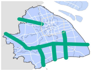 |
| HW_2 km (VC_grass height = 0 m) | 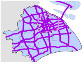 |
| UCM Parameters | UCM Value (High, Low, Industrial–Commercial) | Interpretation |
|---|---|---|
| ALBR | 0.12 | Roof albedo |
| ALBB | 0.15 | Wall albedo |
| ALBG | 0.10 | Road albedo |
| EPSR | 0.85 | Roof emissivity |
| EPSB | 0.9 | Wall emissivity |
| EPSG | 0.95 | Road emissivity |
| AKSR | 1.3 | Conductivity of roof (W/mK) |
| AKSB | 1.3 | Conductivity of wall (W/mK) |
| AKSG | 0.4004 | Conductivity of road (W/mK) |
| CAPR | 1.8 | Heat capacity of roof (MJ/m3K) |
| CAPB | 1.8 | Heat capacity of wall (MJ/m3K) |
| CAPG | 1.0 | Heat capacity of road (MJ/m3K) |
| ZR | 20 | Roof height (m) |
| ROOF_WIDTH | 20 | Roof width (m) |
| ROAD_WIDTH | 20 | Road width (m) |
| SDZR | 4 | Standard deviation of roof height (m) |
| AH | 90 | Anthropogenic heat (W/m2) |
| ALH | 20.0, 25.0, 40.0 | Anthropogenic latent heat (W m2) |
| Wind Speed | Wind Direction | ||||
|---|---|---|---|---|---|
| Evaluation Methods | Root Mean Square Error (RMSE) | Mean Bias (MB) | Index of Agreement (IOA) | Mean Gross Error (ME) | Mean Bias (MB) |
| Summer | 1.44 | −0.22 | 0.85 | 44.05 | −0.26 |
| Winter | 1.46 | −0.13 | 0.85 | 68.49 | −0.20 |
| Simple Threshold | ≤2 m/s | Absolute Value of ≤0.5 m/s | ≥0.6 | ≤30 degrees | Absolute Value of ≤10 degrees |
| Complex Threshold | ≤2.5 m/s | Absolute Value of ≤1.5 m/s | N/A | ≤55 degrees | N/A |
| Factors | AVE10_UCM | AVE10_HW02 | Change % | XJH_UCM | XJH_HW02 | Change % | Unit |
|---|---|---|---|---|---|---|---|
| WindSpeed | 3.53 | 3.46 | −1.74 | 3.50 | 3.33 | −4.80 | m/s |
| PBL | 470.81 | 406.11 | −13.74 | 510.46 | 414.32 | −18.83 | m |
| Deposition | 46.99 | 38.78 | −17.47 | 58.35 | 38.07 | −34.76 | μg/m2/h |
| PM2.5 | 31.28 | 46.52 | 48.71 | 15.05 | 56.43 | 274.91 | μg/m3 |
Publisher’s Note: MDPI stays neutral with regard to jurisdictional claims in published maps and institutional affiliations. |
© 2021 by the authors. Licensee MDPI, Basel, Switzerland. This article is an open access article distributed under the terms and conditions of the Creative Commons Attribution (CC BY) license (https://creativecommons.org/licenses/by/4.0/).
Share and Cite
Liu, C.; Shu, Q.; Huang, S.; Guo, J. Modeling the Impacts of City-Scale “Ventilation Corridor” Plans on Human Exposure to Intra-Urban PM2.5 Concentrations. Atmosphere 2021, 12, 1269. https://doi.org/10.3390/atmos12101269
Liu C, Shu Q, Huang S, Guo J. Modeling the Impacts of City-Scale “Ventilation Corridor” Plans on Human Exposure to Intra-Urban PM2.5 Concentrations. Atmosphere. 2021; 12(10):1269. https://doi.org/10.3390/atmos12101269
Chicago/Turabian StyleLiu, Chao, Qian Shu, Sen Huang, and Jingwei Guo. 2021. "Modeling the Impacts of City-Scale “Ventilation Corridor” Plans on Human Exposure to Intra-Urban PM2.5 Concentrations" Atmosphere 12, no. 10: 1269. https://doi.org/10.3390/atmos12101269
APA StyleLiu, C., Shu, Q., Huang, S., & Guo, J. (2021). Modeling the Impacts of City-Scale “Ventilation Corridor” Plans on Human Exposure to Intra-Urban PM2.5 Concentrations. Atmosphere, 12(10), 1269. https://doi.org/10.3390/atmos12101269