Abstract
The use of low air quality networks has been increasing in recent years to study urban pollution dynamics. Here we show the evaluation of the operational Aburrá Valley’s low-cost network against the official monitoring network. The results show that the PM2.5 low-cost measurements are very close to those observed by the official network. Additionally, the low-cost allows a higher spatial representation of the concentrations across the valley. We integrate low-cost observations with the chemical transport model Long Term Ozone Simulation-European Operational Smog (LOTOS-EUROS) using data assimilation. Two different configurations of the low-cost network were assimilated: using the whole low-cost network (255 sensors), and a high-quality selection using just the sensors with a correlation factor greater than 0.8 with respect to the official network (115 sensors). The official stations were also assimilated to compare the more dense low-cost network’s impact on the model performance. Both simulations assimilating the low-cost model outperform the model without assimilation and assimilating the official network. The capability to issue warnings for pollution events is also improved by assimilating the low-cost network with respect to the other simulations. Finally, the simulation using the high-quality configuration has lower error values than using the complete low-cost network, showing that it is essential to consider the quality and location and not just the total number of sensors. Our results suggest that with the current advance in low-cost sensors, it is possible to improve model performance with low-cost network data assimilation.
1. Introduction
Particulate matter (PM) is one of the most problematic pollutants in urban air [1]. The effects of PM on human health, associated especially with PM of ≤2.5 μm in diameter, include asthma, lung cancer and cardiovascular disease [2]. Consequently, major urban centers commonly monitor PM2.5 as part of their air quality management strategies. There are several techniques to measure the PM concentration in the air, such as filter-based gravimetric method (GMM), β-attenuation absorption method (BAM), and laser-based optical method [3]. The filter-based GMM is the most accurate method but requires parallel processing of blank and sample filter performed in laboratory conditions, and thus is difficult for field application [4]. The BAM PM analyzers employ the absorption of beta radiation by solid particles extracted from air flow [3]. These analyzers have gone through strict field evaluations and demonstrated that they could provide concentration measures equivalent to the filter-based GMM, with the advantage of being usable for continuous PM monitoring (generally with a temporal resolution of 1 h) [5]. Finally, the optical sensors measure particles’ size by light scattering, so the concentration of PM can be detected according to the signal [3,6,7]. The optical sensor’s accuracy is affected by different factors, such as aerosol characteristics, temperature, humidity, and even seasonal types [3]. PM based optical sensors are preferred in large scale commercial sensors due to their affordable cost, low power requirements, and fast response time [6,7].
Public air quality monitoring networks often consist of fixed measuring stations equipped with BAM sensors, and are maintained under rigorous operational and calibration regimes in order to provide high-quality data. The high costs associated with establishing and maintaining such stations means that not all cities in developing countries can afford monitoring networks of sufficient spatial coverage [8]. Even in large cities in developed countries, the official air quality monitoring networks do not always provide information at the spatial and temporal resolution required to assess the impact of pollution sources on health [9], as the cost of the equipment makes the necessary density prohibitive. This has motivated the expansion of low-cost systems and programs to measure PM [10]. The limited number of studies that have evaluated newer generations of optical low-cost PM2.5 sensors have shown that the most widely used sensors attain high accuracy when compared to standard monitoring stations (R2 value ranging from 0.93 to 0.95) [11]. The data provided by these sensors can complement those generated by conventional systems, increasing the data resolution and allowing studies of exposure at the human level [9,12].
The integration of observations from dense networks of low-cost sensors into mathematical models through techniques such as data fusion or data assimilation enables a spatially continuous representation of concentration fields with significantly reduced bias [13]. These techniques provide an added value to the sensor observations by spatially interpolating between monitoring locations and at the same time adding value to the model by constraining the model with observations. Both sources of information can thus be combined in a mathematically objective manner with the goal of reducing the uncertainty inherent to both sources [11,12,14]. Although data assimilation is a more complex family of methods than data fusion or interpolation techniques, it is by far the most versatile and robust of these approaches [13].
This work seeks to implement the data assimilation technique Ensemble Kalman Filter (EnKF) [15] to integrate data from a hyper-dense, low-cost PM2.5 measuring network operated in Medellín (Colombia) and its neighboring municipalities of the Aburrá Valley [16] into the Chemical Transport Model Long Term Ozone Simulation-European Operational Smog (LOTOS-EUROS) [17]. Data generated by the robust, official network of air quality monitoring stations in the Aburrá Valley were previously used for data assimilation in LOTOS-EUROS for modelling and forecasting PM dynamics in the valley [18]. The goal with using data from the low-cost sensor network is to evaluate the impact of hyper-dense observations in the data assimilation approach and their viability as an alternative to monitoring PM2.5 concentrations in developing countries. This study differs from previous studies such as [9,12,14,19], in which a dispersion model was used to construct concentration maps or to estimate emissions from the measured concentration fields, and the integration of the model and observations was based on Kriging or other static approaches. In this work a dynamic data assimilation method is implemented to guide the model’s concentration fields using the observations.
The main contributions from this work are as follows: (1) an evaluation of the low-cost sensor network against the official network; (2) the implementation of techniques for the assimilation of low-cost high-density data, focusing on the impact on the assimilated model results; and (3) a methodology for performing and evaluating PM forecasts with assimilated data over 3-day windows, providing valuable information for decision makers.
2. Materials and Methods
The period of interest for all data evaluations, simulations and data assimilation experiments spans from 25 February to 15 March 2019. During these days, the PM concentrations were higher than usual due to the Northbound transit of the Inter-Tropical Convergence Zone.
2.1. Hyper-Dense Low-Cost Sensor Network
In Medellín and its greater metropolitan area inside the Aburrá Valley, the Sistema de Alerta Temprana del Valle de Aburrá (SIATA) project operates the official high-end air quality monitoring network (henceforth official network), and a hyper-dense, low-cost air quality network developed within the Citizen Scientist program (henceforth low-cost network).
The official network provides high quality measurements for different pollutants in the atmosphere over the Aburrá Valley such as O3, SO2, PM10, PM2.5 and PM1. The official network is distributed among the 10 municipalities of the valley, with the majority of the stations located within the city of Medellín (Figure 1, panel a). The PM measurement equipment consists of Met One Instruments BAM-1020 and BAM-1022 that produce averaged hourly data [16]. The low-cost network was created with the aim of engaging the community in issues surrounding air quality, and as an extension of the official network. As of writing, the low-cost network consists of 255 real-time PM2.5 sensors across the Aburrá Valley and its surrounding hills. The sensors are located in the premises of private homes and public or private institutions (Figure 1, panel b). The measuring equipment was developed by SIATA based on the well-known laser-based optical Shinyei PPD42NS, NOVA SDS011, and Bjhike HK-A5 sensors [16]. The description of the network deployment is presented in [16]. Data were downloaded from SIATA’s data portal (available at https://siata.gov.co/descarga_siata/index.php/index2/. Last accessed, December 2020). Data from the official network for the corresponding dates were used for validation of both the low-cost network and the model simulations before and after data assimilation. Each station from the official network served as a reference point for all low-cost network sensors within a 2-km radius of the former. Performance of the latter was evaluated using as metrics the Mean Fractional Bias (MFB), the Root Mean Square Error (RMSE) and the Pearson correlation coefficient (R) [20,21,22]. When a low-cost sensor had more than one official station within a 2-km radius, the average value of the official measurements was used.
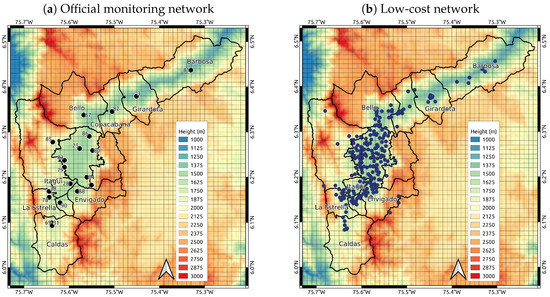
Figure 1.
Spatial distribution of the hyper-dense low-cost network Citizen Scientist and official monitoring air-quality network for particulate matter (PM)2.5. The gray raster represent the Long Term Ozone Simulation-European Operational Smog (LOTOS-EUROS) model grid, the black lines are the boundaries of the municipalities borders, and the numbers are the official station numerations followed by SIATA.
2.2. Particulate Matter Modelling
2.2.1. LOTOS-EUROS Model
Long Term Ozone Simulation-European Operational Smog model (LOTOS-EUROS) [23] is a chemical transport model that simulates concentrations of gasses and aerosols in the lower troposphere on a 3D grid. The simulated species include ozone, nitrogen oxides, volatile organic compounds, secondary inorganic aerosols, dust, and sea-salt [24]. The dynamics are regulated by processes such as chemical reactions, diffusion, drag, dry and wet deposition, emissions and advection [25].
Simulations were conducted using a one-way nested domain configuration as shown in Figure 2 and detailed in Table 1. The innermost domain (D4), the focus of the present study, covered the Aburrá Valley with a model resolution of 0.01° (about 1 × 1 km) as shown in Figure 1. The anthropogenic emissions input for D4 was updated with a high-resolution local emissions inventory constructed as described in Section 2.2.2. The model setup is summarized in Table 2 (for details, see [18]).
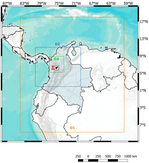
Figure 2.
Nested domain configuration for LOTOS-EUROS simulations. The detailed description of the domains is shown in Table 1.

Table 1.
One-way nested domain configuration used for simulations in LOTOS-EUROS. All data assimilation experiments were conducted in D4.
Table 2.
LOTOS-EUROS simulations setup. LOTOS-EUROS outputs were written hourly. Meteorological data had a temporal resolution of 3 h.
2.2.2. Local Emissions Inventory
An anthropogenic urban emissions inventory for 2016 specific to Medellín and the other nine municipalities of the Aburrá Valley was used for the simulations on the D4 domain. This inventory provides a complete set of emitted trace gases such as carbon monoxide (CO), nitrogen oxides (NOx), sulphur oxides (SOx), and volatile organic compounds (VOCs), as well as particulate matter with diameter less than 2.5 μm (PM2.5) or less than 10 μm (PM10). The construction of the inventory followed a bottom-up methodology, combining activity data (traffic intensities, industrial production) with emission factors. Only traffic and industrial point sources were considered, without accounting for neither household nor commercial emissions [26].
For integration into LOTOS-EUROS, the emission inventory was disaggregated over the Aburrá Valley (76 W–75 W and 5.7 N–6.8 N) at a resolution of 0.01× 0.01 (approximately 1 × 1 km), using a method based on road density as in [27]. The road network map was obtained from the OpenStreetMap database [28], and simplified by removing residential road segments as recommended in [29,30]. The simplification of the road network can reduce errors in the spatial disaggregation since residential roads correspond to a high portion of the road network length but carry a low percentage of total vehicular traffic. For each grid cell j, the corresponding disaggregation factor was calculated as in [27]. Namely,
where is the length of road segment i in the grid cell j, I is the number of road segments in cell j, and J is the total number of grid cells. The point-source emissions were distributed on the grid using their known location, obtained from the official emissions inventory [26]. Figure 3 shows the resulting emissions maps for PM2.5 and PM10.
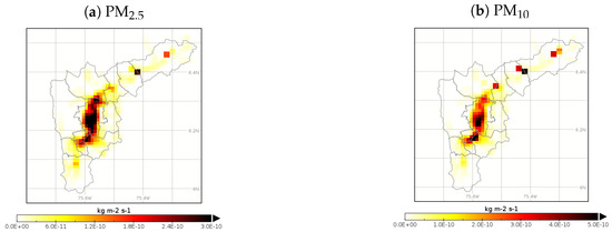
Figure 3.
Local particulate matter emission inventories for the Aburrá Valley: (a) PM2.5, and (b) PM10. The values correspond with the estimated annual emissions.
2.3. Ensemble Kalman Filter
The Ensemble Kalman Filter (EnKF) is a Monte Carlo ensemble method, based on the approximation of the state probability density through an ensemble of model realizations [15]. The EnKF is initialized by generating a random ensemble of model states that represents the model’s uncertainty:
Since emissions are a major source of uncertainty in air quality modelling, we generated the ensembles from perturbations in the emissions. Each ensemble member was propagated in time by the model M to obtain a forecast ensemble:
where is the member of the forecast ensemble at time k. The forecast ensemble describes a stochastic distribution with mean and covariance available from:
with N being the number of ensemble members. The matrix is formed by deviations of the ensemble members from the mean:
Most of the data assimilation applications do not calculate the matrix directly due to its large size. Instead, a consistent square root formulation that only uses and stores is computed [31] in the operational code. The EnKF uses observations to update the forecast ensemble into a corrected or analysis ensemble. Observations collected in a vector are represented as a linear mapping from the state vector plus an observation representation error:
The observation operator H maps the state into the observations. In this application, H selects the concentration in locations where the observations are available. The representation error describes the difference between observation and simulation due to both instrument and sampling errors. is defined as a Gaussian noise with mean 0 and standard deviation depending on the measurement instrument. The analysis ensemble members are calculated as follows:
with
The EnKF system in this application was configured to obtain estimates of both concentrations and emissions. An augmented state vector was used combining the PM2.5 concentrations (c), propagated in time by LOTOS-EUROS, and the emission correction factors (δe), propagated in time by a colored noise model [32]:
where is the LOTOS-EUROS model, and are the correlation length and variance of the stochastic process, and is a standard white noise sample. The emissions () were calculated as:
where represents the nominal emissions from the emissions inventory. For all the simulations we used a τ of 1 day and a σ of 0.5 following previous results [18]. Additionally, we used a covariance localization scheme to reduce spurious correlations among distant states. The covariance localization technique artificially reduces the covariance between states that are separated by longer distances than a threshold radius ρ [33,34]. The parameter ρ defines the area of influence of a given observation on the concentrations and emissions to be estimated. We defined a localization radius ρ = 5 km for all the simulations. We used an ensemble of N = 25 members. Additional experiments with larger ensembles were performed without improvements in performance (not shown).
Two sets of low-cost sensors data were assembled: The first one included 255 sensors from the low-cost network that had a station from the official network within a 2-km radius. The second, higher quality one consisted of a subset of the previous set, including only those sensors whose data showed an R value equal or greater than 0.8 when evaluated against the official network.
We performed four different LOTOS-EUROS simulations:
- a LOTOS-EUROS model simulation without data assimilation (henceforth LE);
- a simulation with assimilation of data (observations) from the 14 stations of the official network (henceforth LE-official);
- a simulation with assimilation of the data from the entire low-cost network (henceforth LE-lowcost)
- a simulation with assimilation only of high-quality data from the low-cost network (henceforth LE-lowcost-HQ).
The seven stations from the official network that were not used for data assimilation were used as validation stations for all simulations.
2.4. Forecast Experiments
Data assimilation can improve forecast performance mainly for two reasons: First, if the simulation is initialized with an assimilated field value, initial conditions at the start of the forecast window may be a closer representation of reality than what the model alone may provide; second, the emission correction factors that were included in the assimilation state (10) can be applied to the model during the forecast window to adjust the emissions in the same direction as during assimilation.
Forecasting experiments were conducted to evaluate the capabilities of the model with data assimilation to forecast PM concentrations in the valley up to three days. Simulations were carried out as above, with the assimilation schedule illustrated in Figure 4. Data assimilation was conducted up to the indicated date, with the three subsequent days representing the forecast window. The forecasting window started at 00:00 hours of the first day after the end of data assimilation. To bring the information obtained in the assimilation window into the forecast window, we used the hourly profile of the correction factor calculated from the last 24 h of data assimilation. The experiments continued until all days between 9 March and 13 March (inclusive) had predictions as the first, second and third day of the forecast. The performance of the forecast was evaluated by calculating the Air Quality Index (AQI) according to the ranges established by the Metropolitan Area (available in Spanish https://www.metropol.gov.co/ambiental/calidad-del-aire/Documents/POECA/Plan_de_Acci%C3%B3n_POECA_Metropolitano_2019.pdf. Last accessed, October 2020.) illustrated in Table 3, and comparing it to the AQI observed for the corresponding day. The comparison against the AQI rather than against plain PM concentrations facilitates the interpretation of the model forecast performance by decision makers and the general public. Additionally, this representation affords evaluating the ability of the model to predict warning-triggering episodes (AQI in orange, red or purple levels). Forecasts missing warning-triggering episodes (false negatives) are especially problematic in air quality management because the resulting inaction can lead to human exposure to dangerous concentrations of pollutants.
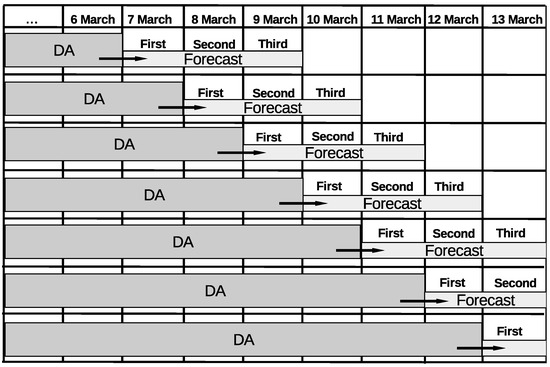
Figure 4.
Graphic explanation of the experimental forecast setup. The arrows represent the inheritance of the last correction factor 24-hourly profile into the forecast. All simulations start at 23 February 19:00 UTC-5. A spin-up period consisting of the 5 days prior to the start date was used for each simulation.
Table 3.
Air Quality Index (AQI) as defined for the Aburrá Valley with respect to PM2.5 concentrations.
3. Results
3.1. Evaluation with Low-Cost Sensor Network
The performance of 145 sensors from the low-cost network was evaluated against data from the official network. The remaining 110 sensors did not have an official monitoring station within a 2-km radius. Figure 5 shows the histograms of the MFB, RMSE and R, and the geographical distribution of the performance values. For the majority (67%) of the low-cost sensors an MFB between −0.25 and 0.25 was obtained, with an average of about 0.2. The average RMSE was close to 8 μg/m3, with most sensors presenting values below 15 μg/m3. The majority (88%) of the sensors showed correlations with R values above 0.7. Observed errors fell within acceptable ranges (as in [21,22]). Zonal differences in measurement errors were observed. Locations in the South-central part of the city of Medellín (green ellipse on Figure 5 d–f) contained most of the sensors with a R values lower than 0.5 and RMSE values grater than 15 μg/m3. Those sensors were located in a dense urban area, while the closest monitoring station is located in the outskirts of the city. Figure 6 shows the spatial distribution of the complete low-cost network and the subset of 115 low-cost sensors with the highest quality data (as defined in Section 2.3). The selection of the low-cost high quality stations was based on the results shown in Figure 5b,e.
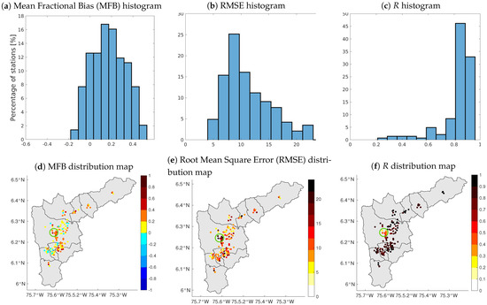
Figure 5.
Evaluation of low-costs network against the official monitoring network for the period between 25 February 2019 and 15 March 2019. Panels (a–c) show the histograms of the MFB, RMSE and R respectively. Panels (d–f) show the MFB, RMSE and R values of each evaluated sensor.
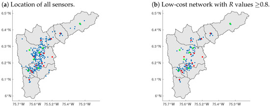
Figure 6.
Spatial distribution of the different sets of sensors (complete network (a) and high-quality network (b) ) used for data assimilation and validation. Blue dots indicate the location of the low-cost sensors. Red squares correspond to the locations of the official monitoring stations that were used for data assimilation. Green stars indicate the stations from the official network whose data where used for validation of all model simulations.
3.2. Evaluation of Data Assimilation Runs
The concentration fields generated by the model simulations with or without data assimilation were compared to the observations from seven of the official monitoring stations (validation stations, green stars in Figure 6) to evaluate the performance of the data assimilation schemes. Figure 7 shows the temporal series for the simulated and observed PM2.5 concentrations at four of the validation stations. The four selected stations represent downtown Medellín (station 25), residential areas (station 86), areas with high vehicular flow (station 88), and a peri-urban area in the outskirts of the city (station 85). Those stations summarize the behavior of all seven validation stations. The LE simulation consistently underestimated the concentrations observed at stations 85 and 88. At stations 25 and 86, the LE simulation results were close in magnitude between 24 February and 3 March and 10 March to 15 March; between 3 March and 10 March, the model presented values much lower than those observed. The day-to-day variability was reduced for this same period, as seen in stations 85 and 86. This inconsistent behavior suggests a poor representation of the meteorological dynamics that governed the dispersion and accumulation of PM2.5 within the valley. Simulations using data assimilation showed noisier behaviors than the LE simulation. This process is commonly observed when applying the EnKF and obeys the stochastic nature and the handling of uncertainty inherent to the method [15]. However, those simulations managed to correct the large discrepancies present in the LE simulation. Both LE-official, LE-lowcost, and LE-lowcost-HQ represented more accurately the day-to-day variability of the observations than LE. In general terms, there was no evidence of a sizeable and persistent difference among the simulations with data assimilation throughout the entire period. Nevertheless, the LE-lowcost-HQ simulation reproduced with greater accuracy the concentrations observed in different periods, such as between 26 February and 4 March in Station 25, between 9 March and 14 March in Stations 85 and 86.
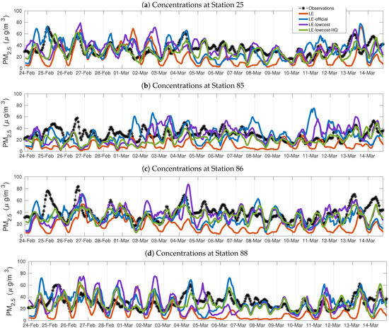
Figure 7.
Temporal series of PM2.5 concentrations from selected validation stations of the official network (a)–(d), LOTOS-EUROS without assimilation, LE-official, LE-lowcost and LE-lowcost-HQ. Time stamps are valid for local time (UTC-5). A spin-up period consisting of the 5 days prior to the start date was used for each simulation.
Figure 8 shows the diurnal cycles during the simulation period in the four selected validations stations. The diurnal cycle of the LE simulation differed from the observations in both magnitude and temporal behavior. The highest concentration peak that appeared around 09:00 in all the stations is mainly due to traffic dynamics. In stations 25 and 88, the LE morning peak corresponded in time but not in magnitude with the observations; in stations 85 and 86, said peak appeared later in the simulations than in the observations. This time lag suggests a poor spatial representation of mobile emissions by the emissions inventory; or a deficiency it the wind fields in reproducing the valley dynamics, showing a late transport of the particulate material to these areas. The LE simulation did not capture the evening peak shown by the observations around 21:00 hours. The simulations using data assimilation presented diurnal cycles closer to the observations than did the LE simulation. The LE-official simulation captured the time and magnitude of the morning peak in stations 85 and 86. In station 88, LE-official corrected the time lag in the morning peak seen in LE, and improved the estimated magnitudes albeit still falling short of the observed values. A different behavior was seen for station 25, where LE-official had low diurnal variability, with a slight underestimation in the morning, and an overestimation in the afternoon. The LE-lowcost and LE-lowcost-HQ simulations results resembled closely the diurnal behavior of the observations, especially the temporal component. In all the stations, both the morning and the evening peaks matched the observations. The observed concentrations for stations 25 and 88 fell inside the standard deviation range for the LE-lowcost simulation; the same simulation overestimated the concentrations between 11:00 and 19:00 for station 85, and underestimated the concentrations between 01:00 and 13:00 for station 86. The LE-lowcost-HQ simulation results were overall the closest to observations.
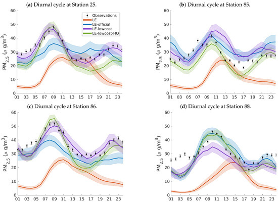
Figure 8.
Diurnal cycle of PM2.5 concentrations from selection stations of the official network (a–d), LOTOS-EUROS without assimilation, LE-official, LE-lowcost and LE-lowcost-HQ. The bars and the shadows represent the standard deviation over the simulation period. The time stamps are valid for local time (UTC-5).
The averaged evaluation statistics among all the validation station are shown in Table 4. The simulation results without data assimilation (LE) underestimated the observed concentrations in all the validation stations. This was also seen in previous related works [18,35]. The RMSE value reflected a low correspondence between the observed and simulated concentrations when using the model without data assimilation. The correlation coefficient was low, meaning that the model was not able to capture the variations in diurnal and day-to-day concentrations. In contrast, the three simulations using data assimilation had MFB values close to 0, without a significant difference among them. The data assimilation was thus effective in reducing the difference between the model and reality. The RMSE also decreased when using data assimilation, by 24.4% in the LE-official, 32.8% in the LE-lowcost, and 36.2% in the LE-lowcost-HQ simulations relative to the RMSE of the LE simulation. The R values were all above the criteria of good performance according with [36] Table 2, and based in [21,37]. Assimilation of either data set from the low-cost network resulted in improved error statistics when compared to the LE-official simulation.
Table 4.
Mean Fractional Bias, Root Mean Square Error and Pearson Correlation Coefficient for simulated PM2.5. Values are averaged over all the validation stations for the simulation period.
3.3. Evaluation of Forecasts
Figure 9 shows a graphical evaluation of the model forecasts for 12 March as Day 1, 2 or 3 within the forecasting window. Forecasts for all other days within the forecasting experiment behaved similarly. The observed AQIs and the values for the LE simulation are the same in all the graphs since all graphs illustrate the same calendar day (12 March). Similar to the results shown in Section 3.2, the LE simulation underestimated PM2.5 concentrations throughout the valley, yielding in most cases AQI lower than those reported. The AQI forecasts of the three simulations with data assimilation were consistently more accurate than the estimates from the simulation without assimilation (LE). There were no significant differences in performance among the three data assimilation simulations through the three forecast days. The forecast accuracy decreased as the forecasting window advanced, as could be expected from the uncertainty inherent in the meteorological fields and nominal emission factors. All three simulations with data assimilation had similar spatial behavior, with a tendency to underestimate the AQI in the Northern and Eastern areas of the valley.
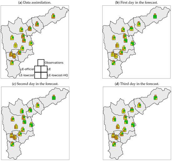
Figure 9.
Evaluation of Air Quality Index (AQI) forecast capabilities of LOTOS-EUROS for the Aburrá Valley. All figures represent the forecasts and analysis for 12 March when it corresponded to analysis day (a), the first (b), second (c) and third (d) day within the forecasting window. The five-square markers are located at the geographical location of each of the official stations used for comparisons. The upper-center square is the AQI calculated from the observed PM values, against which all other values are compared; the middle-left inner square is the AQI predicted by the LE-official simulation; the middle-right inner square is the AQI predicted by the model without assimilation; the bottom-left inner square the AQI predicted by the LE-lowcost simulation; and the bottom-right inner square is the AQI predicted by the LE-lowcost-HQ simulation. The AQI definition is as in Table 3.
For public information on air quality, it is essential that a forecast correctly warns of a critical pollution event. Figure 10 shows the confusion matrix for LE-official, LE-lowcost, and LE-lowcost-HQ simulations in the data assimilation and forecast windows. The confusion matrix summarizes the percentage of true negatives, true positives, false negatives, and false positives [38]. Data assimilation evaluation was performed just in the seven validation stations shown in Figure 6. The LE simulation did not offer a warning in any station in the assimilation nor in the forecast window; for that reason, its confusion matrix is not presented. In the assimilation window, data assimilation simulations have a percentage of true negatives and true positives higher than 80%, and even higher than 90% in the case of the LE-lowcost-HQ. Both simulations using the low-cost network showed lower false negative values than LE-official. The LE-lowcost-HQ had the highest accuracy in reproducing the warning-triggering events within the data assimilation window. The accuracy of the three simulations was lower in the forecast window than in the assimilation window. The small percentage of false positives and high percentage of false negatives suggests that even using the estimated emissions inventory, the simulations continue to underestimate the observations. As observed within the data assimilation window, the two simulations assimilating data from the low-cost network (LE-lowcost and LE-lowcost-HQ) had better warning forecast performance than the LE-official simulation.
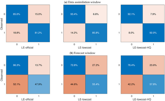
Figure 10.
Comparison of the confusion matrices for the data assimilation (a) and forecast windows (b) depending on warning or no warning per station. The values were calculated across all the days of the corresponding window. A value of 0 corresponds with no warning, while a value of 1 indicates a warning-triggering event. For the LE simulation, there were warnings in neither the data assimilation window nor the forecast windows.
4. Discussion
The results presented herein support the feasibility of using networks of low-cost measuring stations for monitoring air quality in cities such as Medellín. The high spatial density of the low-cost network allowed for a much higher spatial resolution than that attained with the official network. The errors in the low-cost sensors located within the green ellipse in Figure 5d–f represented spatial outliers. The increased errors observed in this sector of the valley may be attributed to specific factors such as maintenance, characteristics of the infrastructure in which the sensors are located, differences in elevation relative to the official station against which they were evaluated, or particular meteorological conditions within the subregion of the valley that may yield local heterogeneity in PM concentrations. Said green ellipse corresponds to a transition zone between peri-urban terrain and an expanding horizon of high-density residential buildings. The low-cost sensors are located in buildings, while the official monitoring station is located in a school surrounded by forests. This may explain the apparent overestimation of the PM levels by the low-cost sensors and the low correlation values of their data.
Our results displayed low correlation values and a marked tendency to underestimate the observed concentrations by the LOTOS-EUROS model without assimilation. Similar behaviors were observed in previous works [18,35]. In [35] the WRF-Chem model in a sub-kilometer configuration was used to reproduce the CO dynamics in the valley. The emission inventory was obtained from the AMVA Official Emission Inventory [26] following a methodology similar to the presented in Section 2.2.2. Although the meteorological fields showed a high similarity with observations, the model underestimated the CO concentrations. The underestimation in both cases is attributed to mismatches in the official emissions inventory and uncertainties generated by the simplifications of disaggregation methodologies, such as the removal of residential road segments. Additionally, the official emissions inventory does not include commercial sources, biogenic sources, and resuspended dust, which can constitute a considerable part of particulate emissions [39]. However, data assimilation notably improved the ability of LOTOS-EUROS to represent the magnitude and dynamics of PM2.5 within the Aburrá Valley. The assimilation of data from the low-cost network improved the correlation between the observed and the simulated concentrations to a greater extent than when data from the sparse official network was assimilated, both in terms of the RMSE and the R values. The errors left in the simulated concentrations after the assimilation of the low-cost network were within the performance goals for PM2.5 representation formulated in [21,22,37,40]. The uncertainty present in the model caused the percentage of predicted warning-triggering events related to high concentration of PM2.5, to decrease to almost one half of the events observed within the forecasting window (Figure 10). Our results highlight the persistent need to improve the inventories of emissions, the meteorological data used as inputs, and to reduce other sources of uncertainty in the model in order to increase forecasting capacity. Nevertheless, the model’s forecasting capacity was increased when observations were assimilated. The greater spatial coverage of the low-cost network contributed significantly to the improvements against the simulations assimilating data from the official network. The higher density of observations also allowed estimating emissions in more detail, as seen in Figure 8. The more detailed emission estimations in turn allowed a better reproduction of the concentrations in the forecast window even in the absence of data assimilation.
Although the LE-lowcost simulation used more observations than the LE-lowcost-HQ simulation (255 and 115, respectively), the location and quality of the additional observations played an important role. The LE-lowcost-HQ was defined using a high similarity criterion to the official network, so it was not as affected by observations with low quality as LE-lowcost. Comparisons between Figure 6a,b revealed that the additional locations do not increase the spacial density considerably relative to the high-quality low-cost subset. Our results suggest that while a high observation density is essential for improving the performance of a model with data assimilation, it is crucial to consider other factors such as the quality of the data and the location of the sensors. Different techniques of observation localization allow optimizing the number of sensors to improve the data assimilation or other data fusion techniques [41,42,43,44]. We highly recommend implementing these techniques in the development of new low-cost monitoring networks. Apart from minimizing the number of sensors and associated costs, the processing of a reduced number of observations requires less computational resources. As an example, the LE-lowcost simulation was 3.2 times slower than the LE-lowcost-HQ using the same computation configuration. Optimization of computational and time resources are especially important for operational systems.
Jointly with previous work [9,12,14,45,46,47], our results can support and motivate the development of future low-cost networks and their integration in data fusion applications. According to the literature, North America, Europe, and China harbor most of the current low-cost implementations, with experimental, citizen, and data dissemination purposes [8,48]. In developing countries, a low-cost network, together with a CTM and data assimilation can provide a valuable first approach to monitoring PM without the high cost of an official air quality network.
5. Conclusions
We present the assimilation of data from a hyper-dense low-cost PM network into the chemical transport model LOTOS-EUROS in a urban setting. The low-cost network provided high quality data comparable to those provided by the official monitoring network. The performance of the model with assimilation of the spatially-dense data from the low-cost network improved both in terms of its representation of the observed dynamics, as well as in its forecast capabilities, highlighting its value as an air-quality management tool. Our results support the idea than with the current advances in the low-cost sensors, it is possible to use low-cost networks and data assimilation to model and predict air quality in urban areas.
Although one of the main advantages of a low-cost networks is the possibility of implementing hyper-dense networks at relatively low costs, it is recommended to prioritize the quality of the data (sensor quality, calibration, maintenance) and the study of optimal localization. High quality data, and the correct number and localization of sensors improves the data assimilation process and minimizes operational and computational costs.
Author Contributions
S.L.-R.: conceptualization, methodology, software, writing—original draft. A.Y.: methodology, software. N.P.: conceptualization, methodology, writing—review and editing. O.L.Q.: conceptualization, methodology, writing—original draft. A.S.: methodology, software, writing—review and editing. A.W.H.: writing—review and editing, supervision. All authors have read and agreed to the published version of the manuscript.
Funding
This research received no external funding.
Acknowledgments
The authors acknowledge the supercomputing resources made available by the Centro de Computación Científica Apolo at Universidad EAFIT (http://www.eafit.edu.co/apolo) to conduct this work.
Conflicts of Interest
The authors declare no conflict of interest.
References
- Liu, H.Y.; Bartonova, A.; Schindler, M.; Sharma, M.; Behera, S.N.; Katiyar, K.; Dikshit, O. Respiratory Disease in Relation to Outdoor Air Pollution in Kanpur, India. Arch. Environ. Occup. Health 2013, 68, 204–217. [Google Scholar] [CrossRef] [PubMed]
- Liu, H.Y.; Dunea, D.; Iordache, S.; Pohoata, A. A Review of Airborne Particulate Matter Effects on Young Children’s Respiratory Symptoms and Diseases. Atmosphere 2018, 9, 150. [Google Scholar] [CrossRef]
- Su, X.; Sutarlie, L.; Loh, X.J. Sensors and Analytical Technologies for Air Quality: Particulate Matters and Bioaerosols. Chem. Asian J. 2020. [Google Scholar] [CrossRef] [PubMed]
- Le, T.C.; Shukla, K.K.; Chen, Y.T.; Chang, S.C.; Lin, T.Y.; Li, Z.; Pui, D.Y.; Tsai, C.J. On the concentration differences between PM2.5 FEM monitors and FRM samplers. Atmos. Environ. 2020, 222, 117138. [Google Scholar] [CrossRef]
- Masic, A.; Bibic, D.; Pikula, B.; Blazevic, A.; Huremovic, J.; Zero, S. Evaluation of optical particulate matter sensors under realistic conditions of strong and mild urban pollution. Atmos. Meas. Tech. 2020, 13, 6427–6443. [Google Scholar] [CrossRef]
- Tagle, M.; Rojas, F.; Reyes, F.; Vásquez, Y.; Hallgren, F.; Lindén, J.; Kolev, D.; Watne, Å.K.; Oyola, P. Field performance of a low-cost sensor in the monitoring of particulate matter in Santiago, Chile. Environ. Monit. Assess. 2020, 192. [Google Scholar] [CrossRef]
- Bai, L.; Huang, L.; Wang, Z.; Ying, Q.; Zheng, J.; Shi, X.; Hu, J. Long-term field evaluation of low-cost particulate matter sensors in Nanjing. Aerosol Air Qual. Res. 2020, 20, 242–253. [Google Scholar] [CrossRef]
- Kumar, A.; Gurjar, B.R. Low-Cost Sensors for Air Quality Monitoring in Developing Countries—A Critical View. Asian J. Water Environ. Pollut. 2019, 16, 65–70. [Google Scholar] [CrossRef]
- Ahangar, F.E.; Freedman, F.R.; Venkatram, A. Using low-cost air quality sensor networks to improve the spatial and temporal resolution of concentration maps. Int. J. Environ. Res. Public Health 2019, 16, 1252. [Google Scholar] [CrossRef]
- Kumar, P.; Morawska, L.; Martani, C.; Biskos, G.; Neophytou, M.; Di Sabatino, S.; Bell, M.; Norford, L.; Britter, R. The rise of low-cost sensing for managing air pollution in cities. Environ. Int. 2015, 75, 199–205. [Google Scholar] [CrossRef]
- Liu, H.Y.; Schneider, P.; Haugen, R.; Vogt, M. Performance assessment of a low-cost PM 2.5 sensor for a near four-month period in Oslo, Norway. Atmosphere 2019, 10, 41. [Google Scholar] [CrossRef]
- Schneider, P.; Castell, N.; Vogt, M.; Dauge, F.R.; Lahoz, W.A.; Bartonova, A. Mapping urban air quality in near real-time using observations from low-cost sensors and model information. Environ. Int. 2017, 106, 234–247. [Google Scholar] [CrossRef] [PubMed]
- Lahoz, W.A.; Schneider, P. Data assimilation: Making sense of Earth Observation. Front. Environ. Sci. 2014, 2, 1–28. [Google Scholar] [CrossRef]
- Popoola, O.A.; Carruthers, D.; Lad, C.; Bright, V.B.; Mead, M.I.; Stettler, M.E.; Saffell, J.R.; Jones, R.L. Use of networks of low cost air quality sensors to quantify air quality in urban settings. Atmos. Environ. 2018, 194, 58–70. [Google Scholar] [CrossRef]
- Evensen, G. The Ensemble Kalman Filter: Theoretical formulation and practical implementation. Ocean Dyn. 2003, 53, 343–367. [Google Scholar] [CrossRef]
- Hoyos, C.D.; Herrera-Mejía, L.; Roldán-Henao, N.; Isaza, A. Effects of fireworks on particulate matter concentration in a narrow valley: The case of the Medellín metropolitan area. Environ. Monit. Assess. 2019, 192, 6. [Google Scholar] [CrossRef]
- Manders, A.M.M.; Builtjes, P.J.H.; Curier, L.; Denier Van Der Gon, H.A.C.; Hendriks, C.; Jonkers, S.; Kranenburg, R.; Kuenen, J.J.P.; Segers, A.J.; Timmermans, R.M.A.; et al. Curriculum vitae of the LOTOS–EUROS (v2.0) chemistry transport model. Geosci. Model Dev. 2017, 10, 4145–4173. [Google Scholar] [CrossRef]
- Lopez-Restrepo, S.; Yarce, A.; Pinel, N.; Quintero, O.; Segers, A.; Heemink, A. Forecasting PM10 and PM2.5 in the Aburrá Valley (Medellín, Colombia) via EnKF based Data Assimilation. Atmos. Environ. 2020, 232, 117507. [Google Scholar] [CrossRef]
- Pournazeri, S.; Tan, S.; Schulte, N.; Jing, Q.; Venkatram, A. A computationally efficient model for estimating background concentrations of NOx, NO2, and O3. Environ. Model. Softw. 2014, 52, 19–37. [Google Scholar] [CrossRef]
- Chai, T.; Draxler, R.R. Root mean square error (RMSE) or mean absolute error (MAE): Arguments against avoiding RMSE in the literature. Geosci. Model Dev. 2014, 7, 1247–1250. [Google Scholar] [CrossRef]
- Boylan, J.W.; Russell, A.G. PM and light extinction model performance metrics, goals, and criteria for three-dimensional air quality models. Atmos. Environ. 2006, 40, 4946–4959. [Google Scholar] [CrossRef]
- Shaocai, Y.; Brian, E.; Robin, D.; Shao-Hang, C.; Schwartz, E.S. New unbiased symmetric metrics for evaluation of air quality models. Atmos. Sci. Lett. 2006, 7, 26–34. [Google Scholar] [CrossRef]
- Mues, A.; Kuenen, J.; Hendriks, C.; Manders, A.; Segers, A.; Scholz, Y.; Hueglin, C.; Builtjes, P.; Schaap, M. Sensitivity of air pollution simulations with LOTOS-EUROS to the temporal distribution of anthropogenic emissions. Atmos. Chem. Phys. 2014, 14, 939–955. [Google Scholar] [CrossRef]
- Sauter, F.; der Swaluw, E.V.; Manders-groot, A.; Kruit, R.W.; Segers, A.; Eskes, H. TNO Report TNO-060-UT-2012-01451; Technical Report; TNO: Utrecht, The Netherlands, 2012. [Google Scholar]
- Van Loon, M.; Builtjes, P.J.H.; Segers, A.J. Data assimilation of ozone in the atmospheric transport chemistry model LOTOS. Environ. Model. Softw. 2000, 15, 603–609. [Google Scholar] [CrossRef]
- UPB; AMVA. Inventario de Emisiones Atmosféricas del Valle de Aburrá–Actualización 2015; Technical Report; Universidad Pontificia Bolivariana–Grupo de Investigaciones Ambientales, Area Metropolitana del Valle de Aburra: Medellín, Colombia, 2017. [Google Scholar]
- Ossés de Eicker, M.; Zah, R.; Triviño, R.; Hurni, H. Spatial accuracy of a simplified disaggregation method for traffic emissions applied in seven mid-sized Chilean cities. Atmos. Environ. 2008, 42, 1491–1502. [Google Scholar] [CrossRef]
- Haklay, M.; Weber, P. OpenStreetMap: User-Generated Street Maps. IEEE Pervasive Comput. 2008, 7, 12–18. [Google Scholar] [CrossRef]
- Tuia, D.; Ossés de Eicker, M.; Zah, R.; Osses, M.; Zarate, E.; Clappier, A. Evaluation of a simplified top-down model for the spatial assessment of hot traffic emissions in mid-sized cities. Atmos. Environ. 2007, 41, 3658–3671. [Google Scholar] [CrossRef]
- Gómez, C.D.; González, C.M.; Osses, M.; Aristizábal, B.H. Spatial and temporal disaggregation of the on-road vehicle emission inventory in a medium-sized Andean city. Comparison of GIS-based top-down methodologies. Atmos. Environ. 2018, 179, 142–155. [Google Scholar] [CrossRef]
- Tippett, M.K.; Anderson, J.L.; Bishop, C.H.; Hamill, T.M.; Whitaker, J.S. Ensemble square root filters. Mon. Weather. Rev. 2003, 131, 1485–1490. [Google Scholar] [CrossRef]
- Jazwinski, A. Stochastic Processes and Filtering Theory; Number 64 in Mathematics in Science and Engineering; Acadamic Press: New York, NY, USA, 1970. [Google Scholar]
- Ott, E.; Hunt, B.R.; Szunyogh, I.; Zimin, A.V.; Kostelich, E.; Corazza, M.; Kalnay, E.; Patil, D.; Yorke, J.A. A local ensemble Kalman filter for atmospheric data assimilation. Tellus 2004, 56, 415–428. [Google Scholar] [CrossRef]
- Sakov, P.; Evensen, G.; Bertino, L. Asynchronous data assimilation with the EnKF. Tellus, Ser. Dyn. Meteorol. Oceanogr. 2010, 62, 24–29. [Google Scholar] [CrossRef]
- Henao, J.J.; Mejía, J.F.; Rendón, A.M.; Salazar, J.F. Sub-kilometer dispersion simulation of a CO tracer for an inter-Andean urban valley. Atmos. Pollut. Res. 2020, 11. [Google Scholar] [CrossRef]
- Mogollón-sotelo, C.; Belalcazar, L.; Vidal, S. A support vector machine model to forecast ground-level PM2.5 in a highly populated city with a complex terrain. Air Qual. Atmos. Health 2020. [Google Scholar] [CrossRef]
- EPA. Meteorological Monitoring Guidance for Regulatory Modeling Applications; Technical Report; U.S. Environmental Protection Agency: Washington, DC, USA, 2000.
- Kohavi, R.; Provost, F. Applications of Machine Learning and the Knowledge. Appl. Mach. Learn. Knowl. Mach. Learn. 1998, 30, 349–354. [Google Scholar]
- Pachón, J.E.; Galvis, B.; Lombana, O.; Carmona, L.G.; Fajardo, S.; Rincón, A.; Meneses, S.; Chaparro, R.; Nedbor-Gross, R.; Henderson, B. Development and evaluation of a comprehensive atmospheric emission inventory for air quality modeling in the megacity of Bogotá. Atmosphere 2018, 9, 49. [Google Scholar] [CrossRef]
- Chang, J.C.; Hanna, S.R. Air quality model performance evaluation. Meteorol. Atmos. Phys. 2004, 87, 167–196. [Google Scholar] [CrossRef]
- Alexanderian, A.; Petra, N.; Stadler, G.; Ghattas, O. A Fast and Scalable Method for A-Optimal Design of Experiments for Infinite-dimensional Bayesian Nonlinear Inverse Problems. SIAM J. Sci. Comput. 2016, 38, A243–A272. [Google Scholar] [CrossRef]
- King, S.; Kang, W.; Xu, L. Observability for optimal sensor locations in data assimilation. Int. J. Dyn. Control. 2015, 3, 416–424. [Google Scholar] [CrossRef]
- Mazzoleni, M.; Alfonso, L.; Solomatine, D. Influence of spatial distribution of sensors and observation accuracy on the assimilation of distributed streamflow data in hydrological modelling. Hydrol. Sci. J. 2017, 62, 389–407. [Google Scholar] [CrossRef]
- Yildirim, B.; Chryssostomidis, C.; Karniadakis, G. Efficient sensor placement for ocean measurements using low-dimensional concepts. Ocean Model. 2009, 27, 160–173. [Google Scholar] [CrossRef]
- Johnston, S.J.; Basford, P.J.; Bulot, F.M.; Apetroaie-Cristea, M.; Easton, N.H.; Davenport, C.; Foster, G.L.; Loxham, M.; Morris, A.K.; Cox, S.J. City scale particulate matter monitoring using LoRaWAN based air quality IoT devices. Sensors 2019, 19, 1209. [Google Scholar] [CrossRef] [PubMed]
- Isakov, V.; Arunachalam, S.; Baldauf, R.; Breen, M.; Deshmukh, P.; Hawkins, A.; Kimbrough, S.; Krabbe, S.; Naess, B.; Serre, M.; et al. Combining dispersion modeling and monitoring data for community-scale air quality characterization. Atmosphere 2019, 10, 610. [Google Scholar] [CrossRef] [PubMed]
- Moltchanov, S.; Levy, I.; Etzion, Y.; Lerner, U.; Broday, D.M.; Fishbain, B. On the feasibility of measuring urban air pollution by wireless distributed sensor networks. Sci. Total Environ. 2015, 502, 537–547. [Google Scholar] [CrossRef]
- Morawska, L.; Thai, P.K.; Liu, X.; Asumadu-Sakyi, A.; Ayoko, G.; Bartonova, A.; Bedini, A.; Chai, F.; Christensen, B.; Dunbabin, M.; et al. Applications of low-cost sensing technologies for air quality monitoring and exposure assessment: How far have they gone? Environ. Int. 2018, 116, 286–299. [Google Scholar] [CrossRef] [PubMed]
Publisher’s Note: MDPI stays neutral with regard to jurisdictional claims in published maps and institutional affiliations. |
© 2021 by the authors. Licensee MDPI, Basel, Switzerland. This article is an open access article distributed under the terms and conditions of the Creative Commons Attribution (CC BY) license (http://creativecommons.org/licenses/by/4.0/).