Analysis on the Evolution and Microphysical Characteristics of Two Consecutive Hailstorms in Spring in Yunnan, China

Abstract

By using products of the cloud model, National Centers for Environmental Prediction (NCEP) Final Operational Global Analysis (FNL) reanalysis data, and Doppler weather radar data, the mesoscale characteristics, microphysical structure, and mechanism of two hail cloud systems which occurred successively within 24 h in southeastern Yunnan have been analyzed. The results show that under the influence of two southwest jets in front of the south branch trough (SBT) and the periphery of the western Pacific subtropical high (WPSH), the northeast-southwest banded echoes affect the southeastern Yunnan of China twice. Meanwhile, the local mesoscale radial wind convergence and uneven wind speed lead to the intense development of convective echoes and the occurrence of hail. The simulated convective cloud bands are similar to the observation. The high-level mesoscale convergence line leads to the development of convective cloud bands. The low-level wind direction or wind speed convergence and the high-level wind speed divergence form a deep tilted updraft, with the maximum velocity of 15 m·s⁻¹ at the −40~−10 °C layer, resulting in the intense development of local convective clouds. The hail embryos form through the conversion or collision growth of cloud water and snowflakes and have little to do with rain and ice crystals. Abundant cloud water, especially the accumulation region of high supercooled water (cloud water) near the 0 °C layer, is the key to the formation of hail embryos, in which q_c is up to 1.92 g·kg⁻¹ at the −4~−2 °C layer. The hail embryos mainly grow by collision-coalescence (collision-freezing) with cloud water (supercooled cloud drops) and snow crystal riming.

1. Introduction

Many studies have shown that the intense convective hail cloud is directly caused by meso- and micro-scale systems under large-scale background circulation. It is greatly affected by local terrain. Meanwhile, it is often accompanied by severe convective weather such as thunderstorms and short-duration heavy precipitation, with characteristics of intense suddenness and locality, short duration, severe disaster, and difficulty in monitoring and forecasting. Therefore, research on the monitoring and early warning technology of hail weather have been undertaken for a long time [1,2,3,4,5]. With the continuous improvement of the detection capability of Doppler weather radars and meteorological satellites in particular, meteorologists have carried out a large number of research projects on the mesoscale features and early identification techniques of severe convective hail weather based on unconventional observation data and have achieved fruitful results [6,7,8,9].

However, due to the limitation of spatiotemporal resolution and coverage of the detected data, it is still difficult to gain a thorough understanding of the evolution and physical structure of convective clouds. It is also difficult to observe the hydrometeor particles in convective clouds directly. It can only be obtained by numerical simulation at present [10,11,12]. As a supplement to the observation data, the numerical model simulation products can provide a detailed and comprehensive understanding of the cloud’s physics processes as well as the distribution and evolution characteristics of the cloud’s physical structure during the formation of the severe convective cloud [13,14,15]. In 1959, Blair [16] published a solution to an unstable stratified two-layer mixed incompressible fluid dynamics equations. Since then, the simulation of shallow convection dry thermal bubbles has become the real basis of cloud simulation research, and research of cloud numerical simulation has become the basic research method of classic theories, observations, and experiments of severe convective weather. Two models are usually used for studying severe convective weather [17]. One is a simple cloud model initiated by artificially adding thermal and cold bubbles, whose simulation scale is small and environmental field is simple. It is mostly used to study the microphysical processes of severe convective clouds [18,19,20], including ice-phase physics processes in the cloud, the mechanism of hail recirculation growth, distribution characteristics of hail particles, etc. Weisman et al. [21] and Kain et al. [22] argued that the Weather Research and Forecasting (WRF) model could reproduce the dominant, larger-scale circulations and hydrometeor fields associated with organized storms and convective systems when it ran at a horizontal grid spacing of 4 km or finer. With the development of atmospheric detection technology, computer technology, and computing methods, more complex cloud microphysical schemes were applied to the mesoscale models, so another mesoscale cloud-resolving numerical model has been rapidly developed, for example, the advanced research version of the WRF model (WRF-ARW) [23]. Due to the consideration of the interactions between the large scale and meso- and micro-scale, the mesoscale cloud-resolving model simulation results can more accurately reflect the occurrence mechanism and laws of severe convective weather. It has become an important method for research on evolution characteristics and microphysical process of severe convective clouds (such as hail clouds) and their monitoring and forecasting. By using a one-dimensional hail growth model within WRF, Adams-Selin et al. [24] showed that when WRF successfully forecasted convection, the hail size forecasted was within 0.5 in. 66% of the time. Kang et al. [25] inferred that the region of formation and growth of hail was in agreement with the intersection of updraft and downdraft by simulation study on the hail cloud microphysical process on the northeastern side of the Qinghai–Tibet Plateau. After the WRF numerical simulation study of hail events and physical structures of hail clouds in central China, Fu et al. [26] argued that an accumulation zone was of great importance to the formation and growth of graupels (hail embryos) and hail. However, Zhang et al. [27] argued that the accretion between graupel and supercooled cloud water and the autoconversion of graupels were the main microphysical mechanisms of hail formation.

Yunnan Province is in the low-latitude plateau of the southwestern border of China. Due to better thermal and humid conditions and complex mountain topography, local severe convective hail weather occurs frequently, and its formation and development are different from other regions. Some studies [28,29,30] on the macroscopic characteristics and formation conditions of hail clouds have been carried out by using conventional or unconventional meteorological observation data. However, the research on numerical simulation and microphysical structural features for hail clouds in Yunnan Province is still blank. On 19 March 2019, the same area in southeastern Yunnan suffered two consecutive severe hail weather attacks within 24 h; the occurrence of big hail in the early morning was especially rare in history. In this paper, by using the cloud model products and Doppler weather radar data, the evolution characteristics, and microphysical structures of convective clouds during this hailfall process are analyzed to reveal the occurrence and development mechanism of hail clouds in the low-latitude plateau.

2. Data and Simulation Methods

2.1. Data

The National Centers for Environmental Prediction (NCEP) Final Operational Global Analysis (FNL) reanalysis data were used to analyze the synoptic background of the hail formation, with the horizontal grid resolution of 1° × 1°, 26 vertical layers, and the time interval of 6 h, including physical quantities of geopotential height, u-wind, v-wind, and vertical velocity. The data from Wenshan Doppler Weather Radar was used to analyze the mesoscale characteristics of hail clouds, with the resolution of 0.3× 0.3 km², the wavelength of 5 cm, and the observation interval of about 6 min. Observation data and hail disaster data were from county weather stations in Yunnan Province.

2.2. Simulation Methods

This research uses the business-as-usual model (Cloud Precipitation Explicit Forecast System), which is coupled with the Chinese Academy of Meteorological Sciences (CAMS) mixed-phase two-moment bulk water microphysical scheme under the WRF dynamic framework. This scheme was developed by Lou et al. [31,32] based on the early convective cloud model and stratiform cloud model of Hu et al. [33,34]. It is a quasi-implicit mixed-phase two-moment microphysical scheme. The model considered 31 cloud-physical processes and contained 56 equations, and adopted a quasi-implicit calculation format to ensure the positive definiteness, stability, and conservation of hydrometeors.

Based on WRF V3.2 mesoscale dynamic framework configured with a two-way nested grid, the physical process used KF-eta cumulus parameterization scheme [22], CAMS cloud-resolving microphysical scheme [31,32,33,34,35], the Yonsei University (YSU) planetary boundary layer (PBL) scheme [36], the Rapid Radiative Transfer Model (RRTM) long-wave radiation scheme [37], and Goddard shortwave scheme [38,39]. The initial and lateral boundary conditions were from the NCEP global forecast system.

The model products include a total of 31 predicted variables, including six types of hydrometeor of water vapor, cloud water, graupel, ice crystals, rainwater, and snow crystals. The horizontal grid resolution is 3 × 3 km², with 19 vertical layers (100~1000 hPa). The model initially ran at 12:00 UTC on 18 March 2019, and the simulation time was 48 h with an interval of 1 h.

3. Hail Process Characteristics

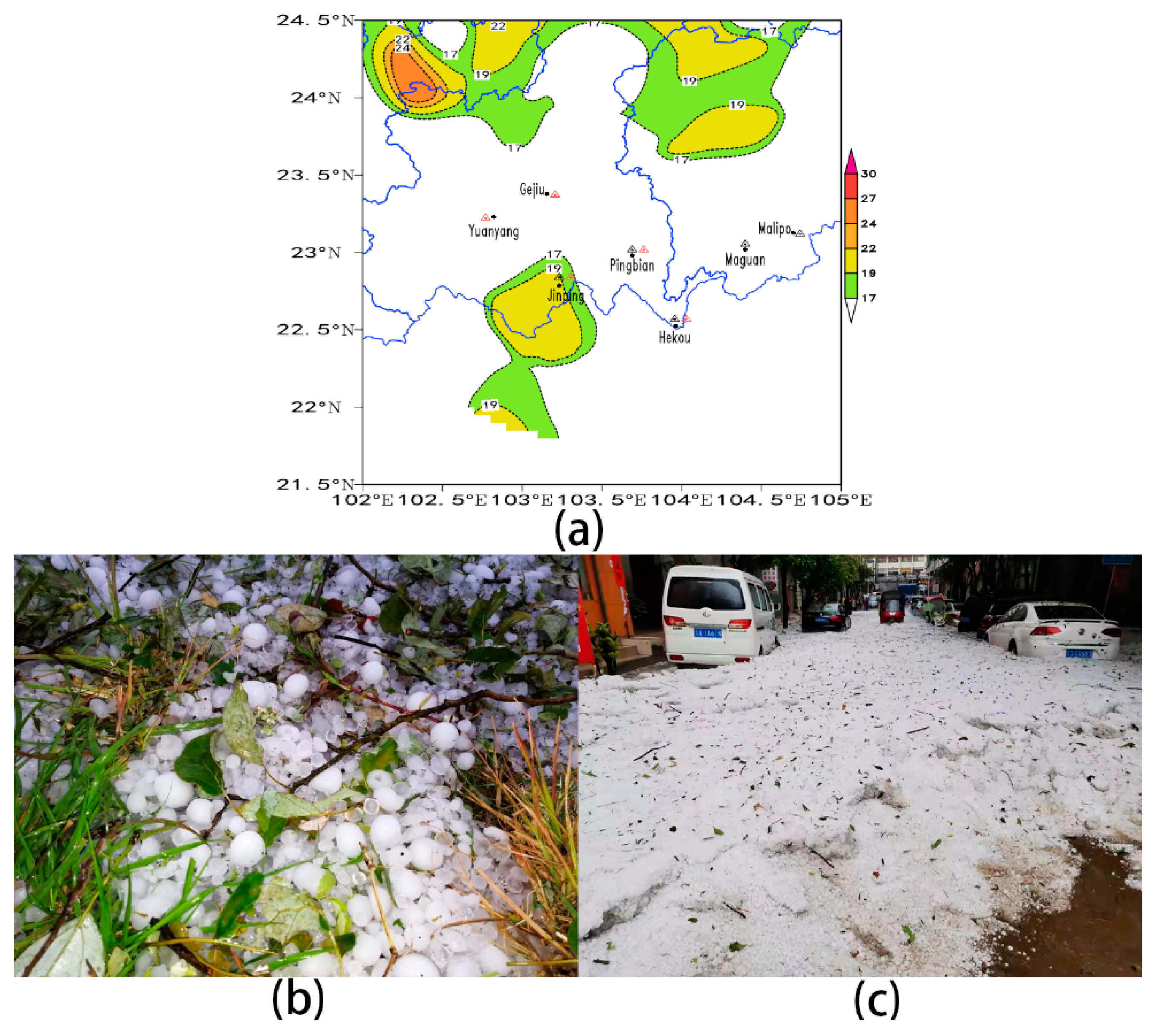
3.1. Synoptic Characteristics

From 18 March 2019 12:00 UTC to 19 March 2019 12:00 UTC, two severe hail processes occurred in southeastern Yunnan Province within 24 h from west to east (Figure 1). The first hail process was from 18 March 2019 22:40 UTC to 19 March 2019 02:00 UTC and occurred in five counties (including Jinping, Pingbian, and Hekou of Honghe Prefecture, Malipo, and Maguan of Wenshan Prefecture), in which the maximum hail diameter was 10 mm in Pingbian and Hekou, and was 30 mm in Jinping County with a maximum wind speed of 19.5 m·s⁻¹ at 21:39 UTC and hourly precipitation at the Kafang Town up to 20.1 mm from 18 March 2019 23:00 UTC to 19 March 2019 00:00 UTC. The second hail process was from 19 March 2019 08:00 UTC to 10:00 UTC and occurred in five counties (including Gejiu, Yuanyang, Jinping, Pingbian, and Hekou of Honghe Prefecture), and the maximum hail diameter also was 30 mm in Jinping County. Therefore, the hail weather was severe and concentrated, with the spatial distribution characteristics of mesoscale weather. Three counties of Jinping, Pingbian, and Hekou were hit by hail disasters twice a day. Among them, the maximum hail diameter was 30 mm and the stacking thickness was about 30 cm in Jinping County, accompanied by the local gale and short-duration heavy precipitation, making it the most severe hail weather in the past 30 years.

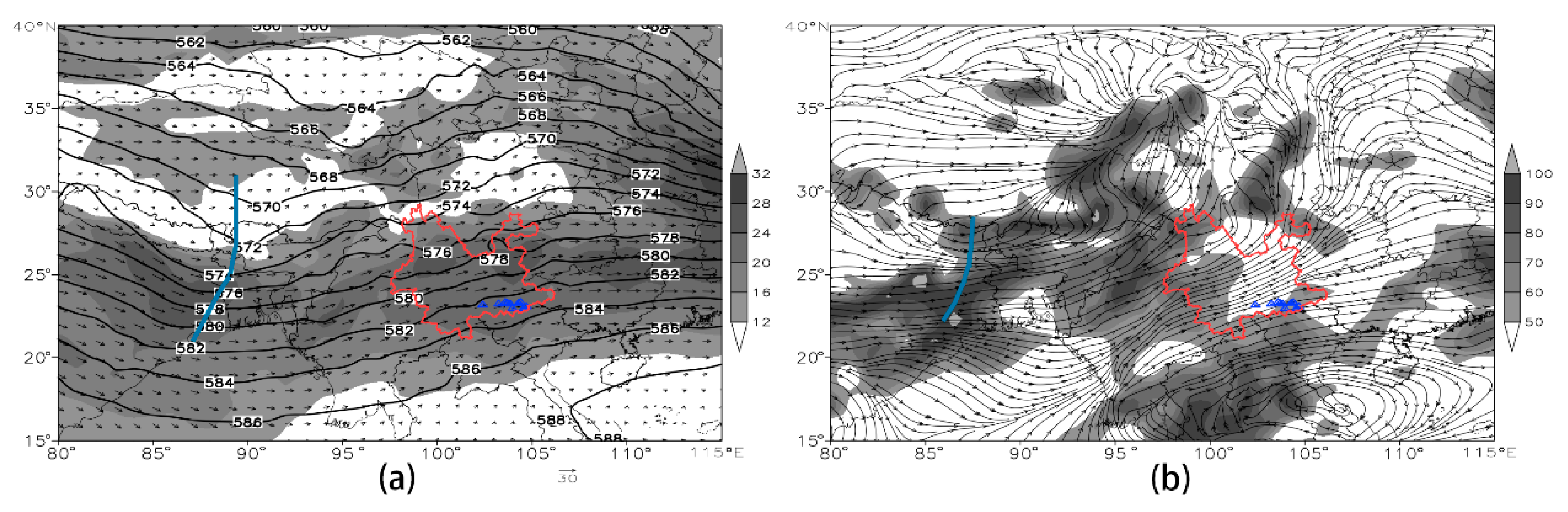
3.2. Synoptic Background

From the 500 hPa geopotential height field and wind field on 18 March 2019 at 12:00 UTC (Figure 2a), the south branch trough (SBT) lies between 85° E and 90° E, the southwesterly jet in front of the SBT traverses the entire Yunnan from west to east, and the wind speed in most parts of Yunnan is ≥24 m s⁻¹. Meanwhile, the 588 dagpm ridge line of the western Pacific subtropical high (WPSH) extends westwards to 107° E and northwards to 18° N. So southern Yunnan is affected by the superposition of two southwest jets simultaneously.

The 700 hPa flow field and relative humidity (RH) distributions (Figure 2b) shows that the SBT also exists between 85° E and 87° E, and Yunnan is affected by southwest-northeast water vapor band in front of the trough. The RH is ≥50% in western Yunnan and ≥70% in local areas. Meanwhile, southern Yunnan is also affected by another southwesterly water vapor transport band in the periphery of WPSH, and the RH is ≥50% at the edge of Southern Yunnan.

Because the wind velocity at 500 hPa is larger than that at 700 hPa, strong vertical wind shear is formed, and the anticyclonic shear on the right side of the high-level jet produces a divergent pumping action. They provide dynamic conditions for hail weather. At the same time, the two low-level southwest airflows continuously transport warm and humid air to provide the moisture and energy conditions for hail weather. The two hail weather processes occurred in the common influence area of two southwest jets, namely the right side (south side) of the high-level southwest jet axis.

3.3. Radar Echo Characteristics

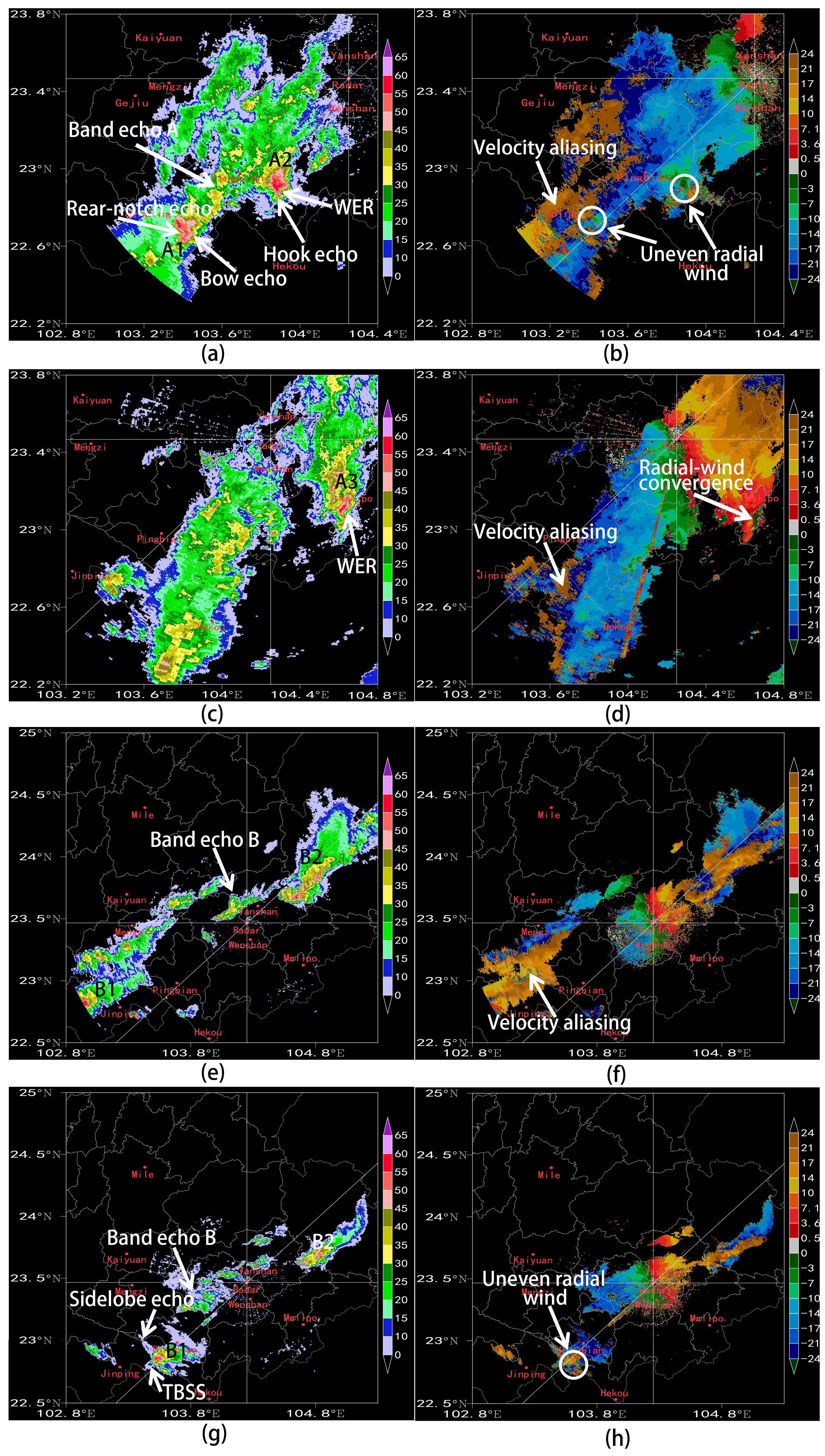
3.3.1. Plan Position Indicator (PPI) Characteristics

(a)

The First Hail Process

As Wenshan radar started to detect at 23:30 UTC on 18 March 2019, there was already a northeast–southwest oriented banded echo A stretching from Jinping, Hekou, Pingbian to Wenshan at 23:40 UTC (Figure 3a). In the radial velocity field (Figure 3b), the zero isodop distribution is in the northwest-southeast direction, and velocity aliasing occurs outside the radius of 75 km, indicating that there is a high-level southwest jet and the wind speed increases with height. The high-level warm and humid airflow and strong vertical wind shear lead to the formation and development of convective echoes. In the eastern (front) banded echo A, that is, in the southeast border of Jinping County and eastern Pingbian County, the radial wind distribution is uneven, indicating the existence of mesoscale convergence and divergence, which is conducive to the intense development of convective echoes of A1 and A2. The reflectivity factor of A1 is 53 dBz, with forward-convex bow-echo and rear notch echo, which is caused by the intrusion of strong downdraft due to precipitation or hail in the rear (west side), resulting in hail and gale weather in Jinping County. The reflectivity factor of A2 is 62 dBz, with a weak echo region (WER) on its front side (southeast side) and with a hook echo on its right rear side (south side). The entrance of low-level warm and humid air is favorable to the development of convective echoes and the occurrence of hail in Pingbian County. At 00:45 UTC on 19 March 2019 (Figure 3c,d), the banded echo A moves eastward to Guangnan, Xichou, Malipo, and Hekou. There is a mesoscale radial-wind convergence in Malipo County on the front side, that is, the radial velocity is negative on the far side of the radar and is positive on the near side. There is a WER on the front side, indicating that the warm and humid airflow enters the cloud from the front side. This causes the convective echo A3 to rapidly develop to 62 dBz, resulting in hail weather in Daping and Yangwan Town of Malipo County.

(b)

The Second Hail Process

Convective echoes appeared again in Honghe and Wenshan Prefecture after 04:00 UTC 19 March 2019, and gradually developed to form a northeast-southwest oriented banded echo B moving eastward. The reflectivity factor (Figure 3e) and the radial velocity (Figure 3f) field at 08:00 UTC shows that the banded echo B is in Jinping, Mengzi, Yanshan, and Guangnan counties, the southwest wind also prevails and increases with height, with the existence of a southwest jet at the high-level. The banded echo is composed of two sections in the north and south. The north section is in Guangnan County with a reflectivity factor of about 55 dBz. The intense convective echo B1 in the south section moves eastward into Jinping County with a reflectivity factor of 56 dBz. At 08:19 UTC (Figure omitted), the banded echo B continues to move eastward. While B1 moves to the northern Jinping county town, and a three-body scattering signature (TBSS) of 5–10 dBz spike-shaped echo appears in the radial direction of the radar on the southwest side, indicating that there are large hail particles in B1 that produce strong scattering. At 09:00 UTC (Figure 3g,h), the northern section B2 of banded echo B gradually weakens, and the intense convective echo B1 in the southern section moves eastward to the junction area of northwestern Jinping and Pingbian County. Due to the existence of mesoscale convergence and divergence caused by the local uneven distribution of radial wind, B1 continues to develop. The reflectivity factor remains 50~56 dBz with the TBSS always existing, and sidelobe echoes appear on the west side. Moreover, due to strong vertical wind shear, the reflectivity factor gradient of the hail cloud is large on the upwind side (southwest end), and it is small and uniform on the downwind side (northeast end). They are conducive to the formation of a tilted updraft and the maintenance and development of convective echoes, resulting in the second hailfall in Jinping County.

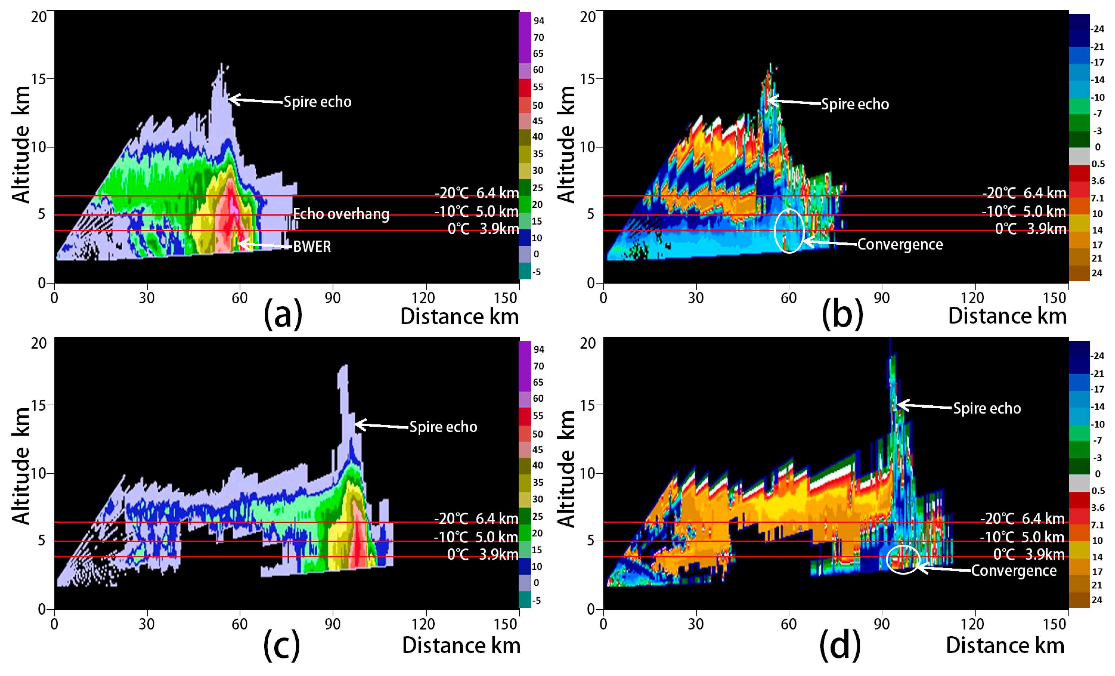
3.3.2. Range Height Indicator (RHI) Characteristics

The range height indicator (RHI) characteristics of the hail cloud reflectivity factor and the radial velocity in the two processes were analyzed in the following. For the 1st hail cloud echo A2 at 00:00 UTC (Figure 4a,b), there is mesoscale radial-wind convergence in the middle-lower level (below 6 km). This is conducive to the entrance of warm and humid air into the cloud and convergence uplift, leading to the formation of a strong echo zone in the middle level of 4.7~6.3 km where the hail grows, with the reflectivity factor of 62 dBz, and 50 dBz height up to 7.3 km (above −10 °C layer). There is a bounded weak-echo region (BWER) below 4.3 km, and the strong echo in the middle level suspends above the lower-level BWER, namely the characteristics of echo overhang. The echo-top height (ETH) is 10.6 km and a spire echo can be observed, indicating that there is the scattering effect of large particles (hail particles) on the radar sidelobes. At 09:00 UTC (Figure 4c,d), the 2nd hail cloud echo B1 between northeastern Jinping and the adjacent area of Pingbian also has mesoscale radial-wind convergence below 5 km, with the ETH up to 12.0 km, the 50 dBz height of 7.0 km, and the characteristic of spire echo.

In summary, the southwesterly wind increases with height forming strong vertical wind shear, resulting in the formation of the northeast–southwest oriented convective banded echoes. On the east and south sides of the convective banded echoes, the convergence of local mesoscale radial-wind or uneven distribution of wind speed is conducive to the entry of warm and humid air from the lower front side into the cloud and convergent uplift. This is conducive to strengthen updraft, leading to the strong development of convective echo and the occurrence of hail. The reflectivity factor is 50–62 dBz, the ETH is 11.0–12.0 km, with the characteristics of low-level WER, hook echo, and middle-high-level echo overhang. Due to the strong scattering effect of large particles (hail), the TBSS and spire echo are produced, while rear-notch echo and bow-echo are formed due to the strong downdraft.

4. Simulation Results

4.1. Hail Cloud Physical Structure Characteristics

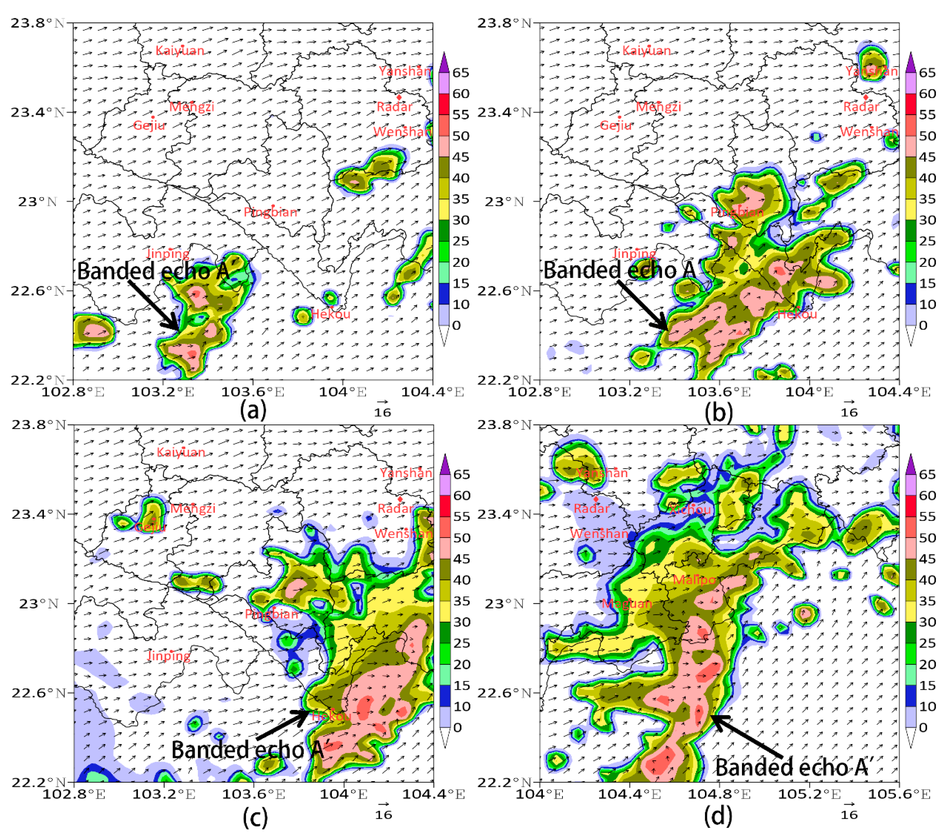
4.1.1. Horizontal Structure

Since the altitude of Wenshan Radar Station is 1775.2 m, the simulation results of 700 hPa reflectivity factor and wind field for two hail processes from 22:00 UTC on 18 March to 01:00 UTC on 19 March (Figure 5) and from 08:00 UTC to 09:00 UTC on 19 March (Figure 6) are selected for analysis respectively.

(a)

The First Hail System

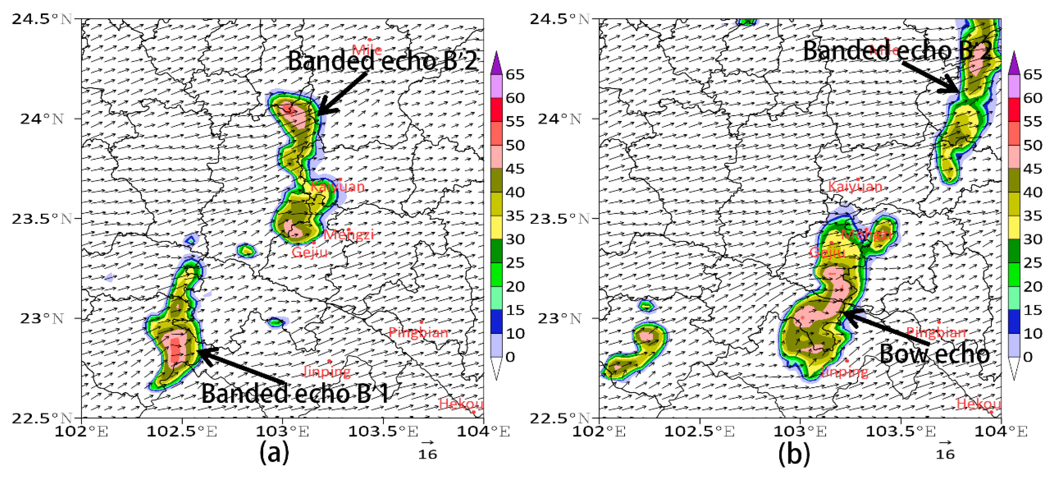
From the simulation result of the first hail process, the southwest wind is prevailing in southeastern Yunnan at 22:00 UTC on 18 March 2019 (Figure 5a). Outside the border of southern Yunnan (within the range of 102.8~103.6° E, 22.0~22.8° N), there are a weak cyclonic bend and southwesterly airflow convergence, which are conducive to water vapor convergence and convection generation. Correspondingly there is a northeast-southwest oriented convective cloud band A’ whose leading edge is close to the south side of Jinping County, with reflectivity up to 50~55 dBz. At 23:00 UTC (Figure 5b), the confluence area of southwest airflow moves northeastward, A’ expands northeast to Hekou and Pingbian County. At 00:00 UTC on 19 March 2019 (Figure 5c), A’ continues to move northeast to Wenshan, Pingbian, Maguan, and Hekou County. There is a mesoscale convergence line of westerly and southwesterly winds between Maguan and Hekou County, leading to the continuous development of the convective cloud band, with the maximum reflectivity factor of 55~60 dBz. At 01:00 UTC (Figure 5d), A’ moves northeast across Malipo and Maguan counties, and the convection near the convergence line between the westerly and southwesterly winds continues to develop.

(b)

The second hail system

From the simulation result of the second hail process, the southwest wind is also prevailing in southeastern Yunnan. At 08:00 UTC on 19 March 2019 (Figure 6a), the convergence of southwesterly and westerly winds respectively exists at the junction of the Lüchun, Jinping, and Yuanyang, and that of Jianshui, Kaiyuan, and Gejiu, leading to the formation and development of two short convection cloud bands of B’1 and B’2 in the south and north. The reflectivity is 45~55 dBz, and the maximum reflectivity is up to 60 dBz. At 09:00 UTC (Figure 6b), the two short bands of convective clouds shift eastward and gradually arrange into discrete cloud band B’ with the northeast-southwest direction. The southern short cloud band B’1 is in the convergence zone between the southerly and the westerly winds, develops more vigorously, and moves eastward to Yuanyang, Gejiu, Mengzi, and Jinping, with the reflectivity factor of 50~55 dBz and the characteristic of the forward-convex bow-echo.

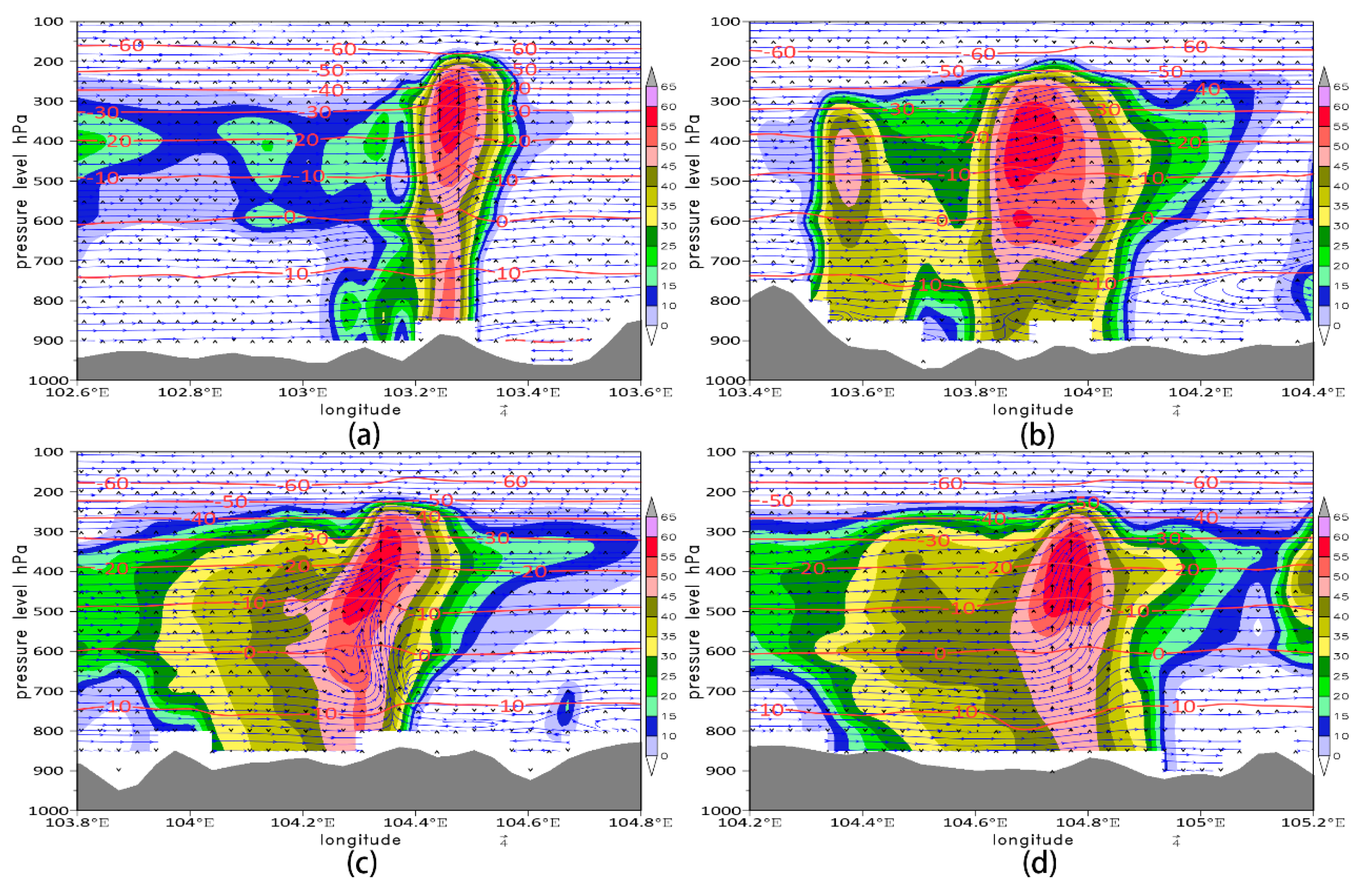
4.1.2. Vertical Structure

The simulation results of the vertical distribution of reflectivity factor, wind field (zonal u wind and vertical w velocity), and air temperature along the high reflectivity center in the two hail processes were analyzed.

(a)

The first Hail System

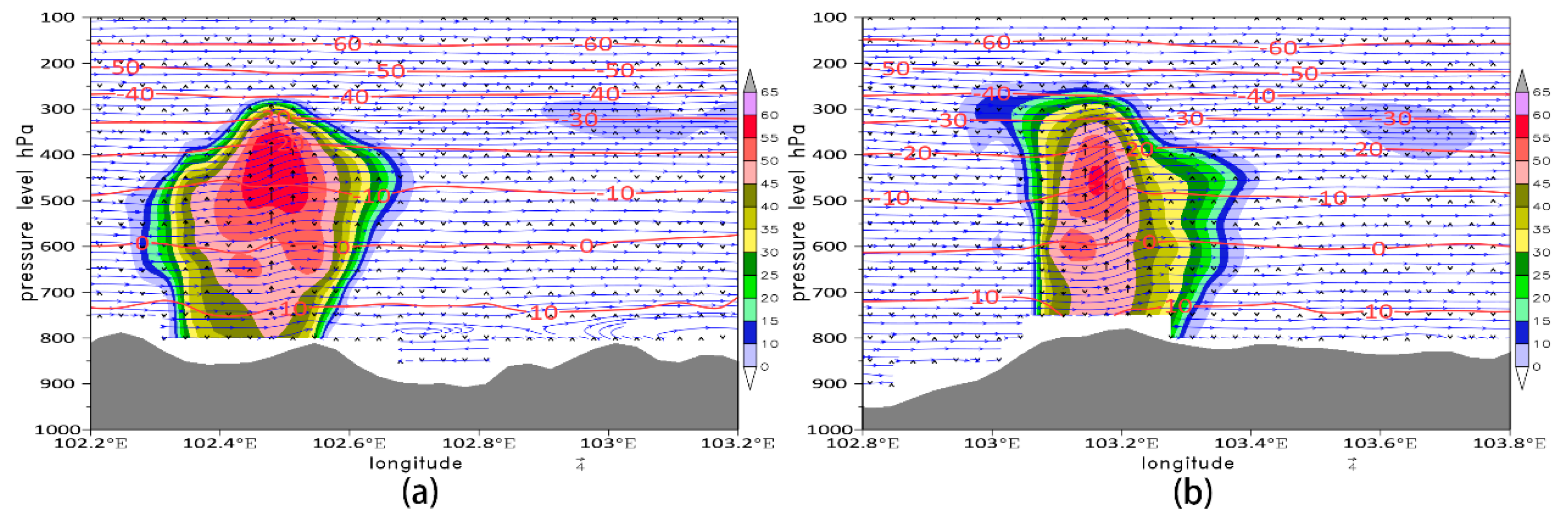
The simulation result of the first hail cloud (Figure 7) shows that the westerly wind is prevailing. At 22:00 UTC on 18 March 2019 (Figure 7a), in the middle-low level (−10~10 °C layer) of the cloud (103.22~103.4° E), there is a convergence of westerly wind speed, namely the wind speed on the rear side (west) is greater than that on the front side (east). In the middle-upper part of the front side of the cloud (−55~−15 °C layer), there is a divergence of westerly wind speed. The low-level convergence and the upper-level divergence on the front side form a strong pumping effect, leading to the enhancing of tilted updraft in the cloud. The updraft in particular is stronger at the −50 °C~0 °C layer, and the strong updraft ≥10 m s⁻¹ appears at the −40~−10 °C layer, with the maximum updraft up to 15 m·s⁻¹ at the −20 °C layer. On the one hand, it is conducive to the low-level water vapor convergence into the cloud and the uplift as well as the condensation growth of hydrometeor particles. On the other hand, it can hold the growing hydrometeor particles, forming large particle accumulation area in the cloud. The cloud-top height (CTH) reaches 13 km (over −60 °C layer). The high reflectivity of 50–60 dBz appears in the strong updraft zone of 220~500 hPa (over −20 °C, reaching −50 °C layer), and the updraft velocity at the high reflectivity center of 60 dBz is ≥8 m s⁻¹. Moreover, due to the latent heat released by the condensation growth of hydrometeor particles in the cloud, the isotherms in the main updraft zone (−20~10 °C layer) in the cloud are convex upward (warming) significantly, and the −10 °C isotherm in particular is up to 1 km compared to the surrounding area.

At 23:00 UTC (Figure 7b), due to the dragging effect of precipitation or hail, a weak downdraft appears below the 0 °C layer, the high reflectivity area of 50–60 dBz extends downward to the −40~4 °C layer. Meanwhile, a high reflectivity center of 60 dBz appears at the 0 °C layer, the CTH is still 13 km, and there are an ice-water mixing area and supercooled cloud-water accumulation area in the cloud. At the same time, the convergence of easterly and westerly winds appears below the 15 °C layer in the cloud, and a weak updraft of 2~4 m s⁻¹ in the middle-upper −45~−5 °C layer still exists.

At 00:00 UTC on 19 March 2019 (Figure 7c), there is a convergence of easterly and westerly winds in the middle to low levels (below −4 °C) of the cloud (104.2~104.4° E). Behind it, there is a convergence of westerly wind speed below the −20 °C layer. In the meantime, there is a divergence of westerly wind speed above the −10 °C layer on its front side. All these are conducive to the low-level warm and humid air converging into the cloud and the uplift and condensation growth of hydrometeors. The tilted updraft from the lower level to the −60 °C layer strengthens, and the maximum updraft (up to 12 m s⁻¹) appears at the front side of the cloud (near 104.34° E) in the mid-upper level (−35~−4 °C layer), leading to the continuous development of the hail cloud. The CTH exceeds 12 km, and the high reflectivity area of ≥50 dBz expands to the −44 °C layer. The 60 dBz high reflectivity center (large particle accumulation area) nears the maximum updraft zone, and a WER appears in the convergence lifting area below the −10 °C layer, with an echo overhang above it, which is conducive to the growth of hail.

At 01:00 UTC (Figure 7d), the convergence of low-level easterly and westerly wind in the cloud weakens and disappears. However, the convergence of westerly wind speed in the middle-low-level and the divergence of wind speed in the upper-middle part (−50~−4 °C layer) of the front side of the cloud still exist. The tilted updraft remains but the tilt reduces, and the updraft of 10 m s⁻¹ is still maintained in the mid-upper level (−28~−10 °C layer), but the intensity and range reduce. The CTH remains at −55 °C layer, but as the high reflectivity area of 50 dBz reduces to the −38~−4 °C layer, the hail cloud weakens.

(b)

The Second Hail System

The simulation result of the second hail cloud (Figure 8) shows that westerly wind is still prevailing from the lower to the upper level. At 08:00 UTC on 19 March 2019 (Figure 8a), there is a convergence of westerly wind speeds below the 0 °C layer on the middle-front side of the cloud (102.4~102.6° E) and divergence of westerly wind speed on the middle-upper part (−35~−5 °C layer) of the front side of the cloud, forming a deep updraft in the −44~15 °C layer, with the maximum updraft of 10 m s⁻¹ at −12 °C layer. Therefore, the area of high reflectivity ≥50 dBz reaches the −30 °C layer along the main updraft. A high reflectivity area of 55~60 dBz forms in the −24~−6 °C layer, that is, the large particle area of the hailstone formation and growth.

At 09:00 UTC (Figure 8b), the updraft is enhanced, the height of strong updraft over 8 m s⁻¹ is close to the −30 °C layer, and the maximum updraft reaches 13 m s⁻¹ at the −18~−8 °C layer. However, the convergence of westerly wind speed in the low level and the divergence of westerly wind speeds in middle-upper level weaken, and the forward-tilted vertical structure of the cloud weakens. At the same time, due to the dragging effect of downdraft caused by falling hail or precipitation below the 0 °C layer on the rear side, the height of the high reflectivity over 50 dBz reduces to below the −25 °C layer. The height of the high reflectivity center of 55–60 dBz in particular reduces significantly and distributes near the −10 °C layer. The hail cloud weakens.

To sum up, the model simulates the structure characteristics of the flow field and vertical wind field of both hail processes well, as well as the intensity, CTH, features, and moving direction of convective cloud bands. The mesoscale convergence line formed by the convergence of high-level southwest airflows or southwest and westerly airflows leads to the formation of convective cloud bands. There is a convergence of low-level easterly and westerly wind or the westerly wind speed, and divergence of high-level westerly wind speeds. This is conducive to the low-level warm and humid air to converge into the cloud and form a strong deep tilted updraft from the lower level to 200 hPa (−50 °C layer), leading to the intense development of local convection. The updraft can reach 12~15 m·s⁻¹ in about a −40~−10 °C layer, especially along the main updraft zone, and the height of high reflectivity over 50 dBz reaches the −40~−50 °C layer, indicating that there may be sufficient supercooled water or accumulation of large particles. The model simulates that the first hail cloud system is stronger than the second, which is consistent with the actual situation.

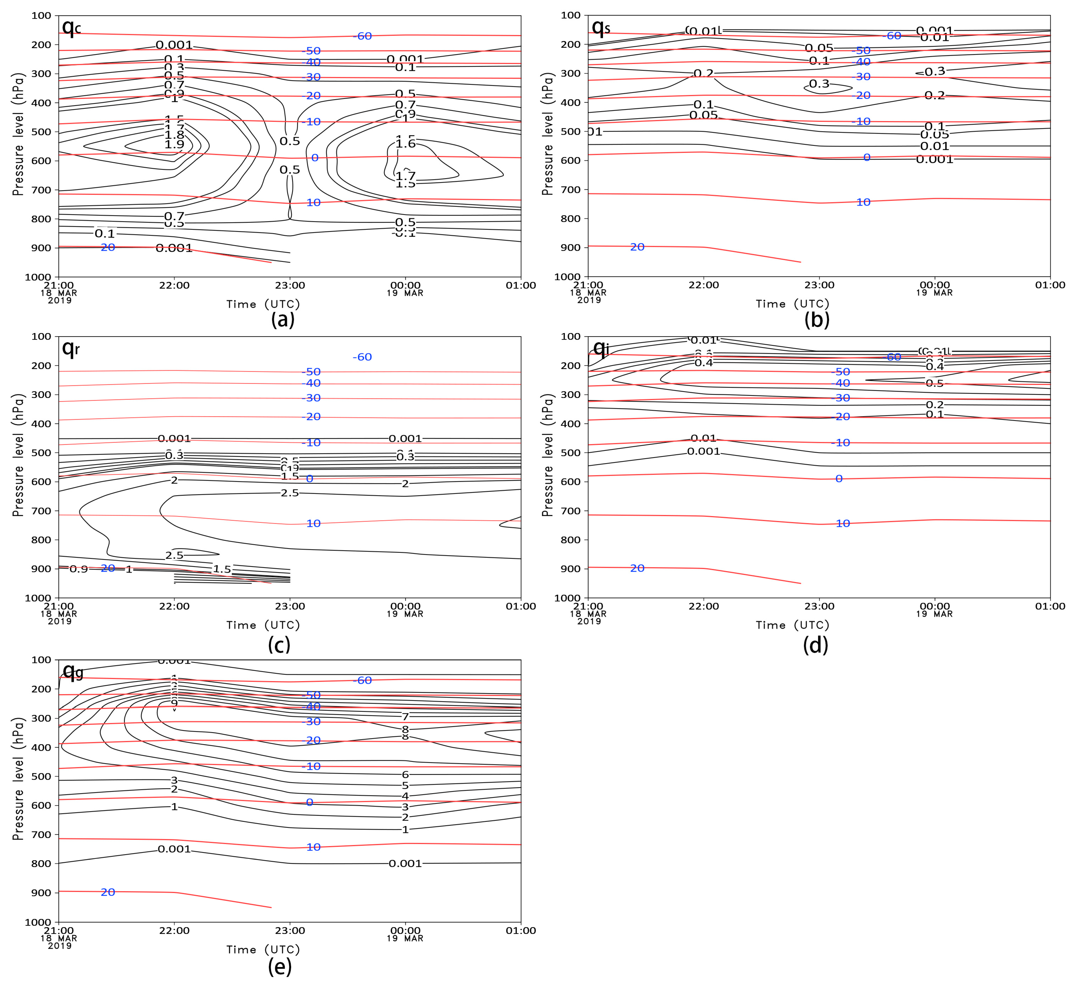
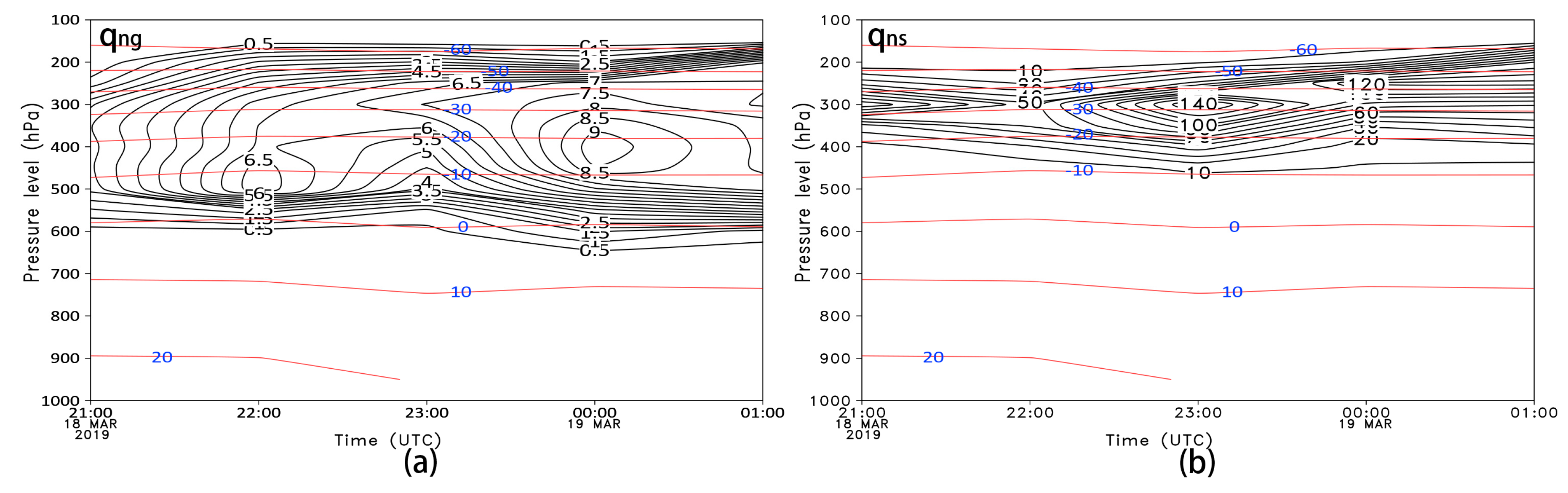
4.2. Distribution Characteristics of Various Hydrometeors

Figure 9 shows temporal-height distributions of the cloud water mixing ratio (q_c), snow mixing ratio (q_s), graupel mixing ratio (q_g), and rainwater mixing ratio (q_r) during the formation and development of the first hail cloud.

The content of cloud water (particularly supercooled cloud water) is rich and deeply distributed (Figure 9a), and concentrates in the −40~15 °C layer. The accumulation area of high supercooled water (cloud water) content is at the −4~−2 °C layer. At 21:00–22:00 UTC on 18 March 2019, the q_c of the whole layers increases rapidly, and the center of high supercooled water content (q_c ≥ 1.6 g·kg⁻¹) appears at the −10 ~ 0 °C layer, with the maximum q_c up to 1.92 g·kg⁻¹ (−2 °C layer) at 22:00 UTC. Possibly due to the latent heat released by the collision-coalescence or collision-freezing growth of hydrometeors, the isotherms are convex upward (warming) in the cloud. At 23:00 UTC, the 10 °C isotherm in the lower layer is concave downward, indicating that the temperature reduces (due to the evaporation or dragging effect) during the falling of hydrometeors (hail or precipitation). The q_c of the whole layer decreases to below 0.5 g·kg⁻¹, a large amount of cloud water is consumed (particularly supercooled cloud water). At 00:00 UTC on 19 March 2019, q_c increases again below the −20 °C layer, and the maximum q_c reaches 1.72 g·kg⁻¹ near the 5 °C layers, which is closely related to the continuous development of the hail cloud.

The q_s is one order of magnitude smaller than q_c (Figure 9b). The distribution height of snow crystals is at the −60~−2 °C layer and higher than that of cloud water, and its accumulation zone appears at the −34~−20 °C layer, corresponding to the maximum updraft zone analyzed previously. The snow crystals gradually increase from 18 March 2019 21:00 UTC, the high-value region of qs ≥ 0.1 g·kg⁻¹ appears at the −43~−18 °C layer, and the maximum q_s reaches 0.28 g·kg⁻¹ near the −35 °C layer. At 22:00 UTC, the vertical distribution range of q_s high-value reduces, and the q_s maximum is only 0.2 g·kg⁻¹ near the −32 °C layer, indicating that a large number of snow crystals are accreted by graupel during the hail growth, or some snow crystals melt due to the release of latent heat during the collision-freezing growth of hail. At 23:00 UTC, as the updraft weakening, the high q_s center expands downward, and the q_s increases, with q_s ≥ 0.3 g·kg⁻¹ in the −30~−20 °C layer, and the maximum q_s of 0.32 g·kg⁻¹.

The rainwater distributes below the −10 °C layer (Figure 9c), and its accumulation zone locates below the cloud water accumulation zone and below 0 °C. It is mainly warm rainwater. From 21:00 to 23:00 UTC, the rainwater increases gradually and continues to expand downward. The q_r increases to more than 2.0 g·kg⁻¹ in the 2~18 C layers at 22:00 UTC, with the maximum q_r of 2.59 g·kg⁻¹ at the 9 °C layer and the second-largest q_r of 2.57 g·kg⁻¹ is near the 18 °C layer. Later the region of q_r ≥ 2.0 g·kg⁻¹ reaches the surface, with the maximum q_r of 2.86 to 2.98 g·kg⁻¹.

The ice crystal accumulation zone is in the −60~−30 °C layer and at the top of the updraft (Figure 9d); q_i is similar to q_s and is one order of magnitude smaller than other hydrometeors. The maximum of q_i is 0.28 g·kg⁻¹ at the −35 °C layer on 18 March 2019 at 21:00 UTC. During 22:00–23:00 UTC, the high-value center of q_i ≥ 0.4 g·kg⁻¹ maintains in the −55~−38 °C layer, and the maximum of q_i is about 0.49 g·kg⁻¹. At 01:00 UTC on 19 March 2019, the q_i maximum is 0.64 g·kg⁻¹ near the −43 °C layer. To sum up, the ice crystals gradually increase in the −55~−38 °C layer during the whole process, and their distribution location is relatively high and changes little, so they have less contribution to the formation and development of hail.

The graupels are mainly in the deep vertical range of the −60~10 °C layer (Figure 9e), and the accumulation zone of q_g ≥ 5 g·kg⁻¹ is in the −50~−6 °C layer. At 21:00 UTC, the high-value center of q_g is 3.94 g·kg⁻¹ at the −18 °C layer. At 22:00 UTC, the region of q_g ≥ 5 g·kg⁻¹ rapidly expands upward and downward to the −50~−10 °C layer, and the maximum of q_g reaches 9.06 g·kg⁻¹ at the −42 °C layer, which is corresponding to the time when the q_s reduces significantly near the −30 °C layer, indicating that snow crystals consume during the rapid increase of q_g. At 23:00 UTC, the region of q_g ≥ 5 g·kg⁻¹ continues to expand down to the −7 °C layer, and the maximum of q_g reaches 8.72 g·kg⁻¹ at the −25 °C layer. It is also the time when q_c reduces significantly in the −20~10 °C layer, indicating that the collision-freezing of a large number of cloud water (particularly supercooled cloud water) particles forms graupels and results in the increase of q_g and decrease of q_c. It also corresponds to the phase of q_s increases and downward expansion, indicating that snowflakes contribute a lot to the formation and growth of graupels. At 00:00 UTC on 19 March 2019, although the vertical distribution range of q_g ≥ 5 g·kg⁻¹ maintains, the vertical distribution of q_g ≥ 8 g·kg⁻¹ significantly reduces from the −33~−18 °C layer to the −26~−23 °C layer.

Meanwhile, the evolution trend of graupel is the same as that of rainwater (warm rainwater), and the vertical distribution of the hail accumulation region is above that of the rainwater, which is closely related to the hail melting and the short-term heavy precipitation accompanying during hailfall.

Therefore, in this hail process, the formation of graupels is closely related to the content of cloud water and snow crystals, but not to rain and ice crystals.

Further analyzing the relationship between graupel number concentration (q_ng) and snow number concentration (q_ns) (Figure 10), the maximum q_ns reaches 9.8 × 10⁴·kg⁻¹ (at the −35 °C layer) at 21:00 UTC and decreases to 5.4 × 10⁴·kg⁻¹ (at the −32 °C layer) at 22:00 UTC. The maximum q_ng increases rapidly from 3.0 × 10³·kg⁻¹ at the −25 °C layer to 6.9 × 10³·kg⁻¹ at the −6 °C layer from 21:00 UTC to 22:00 UTC, which has more than doubled. However, the height of the high q_ng center is lower, which is in the same temperature layer as the high q_c center at the same time. Therefore, the snow crystals have been lost in both quality (size) and quantity (number) during the hail formation in the early stage, and graupels mainly form through cloud water freezing or collision with a small number of snow crystals, or the autoconversion of snow crystals. In the later stage, the q_ns increases rapidly at 23:00 UTC, with the maximum q_ns up to 1.4 × 10⁵ · kg⁻¹ near the −30 °C layer, indicating that more snow crystals can participate in the formation of graupels in the upper level. At the same time, the high q_ng center moves up, and the maximum value reaches 7.0 × 10³ kg⁻¹ in −32 °C layer at 23:00 UTC.

In summary, hail embryos (graupels) are formed by the autoconversion or collision-coalescence growth of cloud water and snow crystals. In the early stage of hail cloud formation, the rich and deep cloud water particles grow to form hail embryos by continuous uplift-condensation and collision-coalescence or by collision-freezing with a small number of snow crystals along the deep updraft. In the later stage of development, more falling snow crystals grow to form hail embryos through the accretion or the collision-freezing with supercooled cloud droplets. Therefore, abundant cloud water at the −40~15 °C layer, particularly the high supercooled cloud water accumulation area with q_c of 1.92 g·kg⁻¹ at the −4~−2 °C layer, is the key to the formation of hail embryos in this process. However, snow crystals make some contributions to the formation and increase of hail embryos, but the effect time is later than that of supercooled cloud water, namely, the hail embryos’ increase in hail cloud are firstly contributed by supercooled cloud water, both q_c and q_ng reach a high value in the same layer at the same time, and then, with the participation of more snow crystals, the high q_ng and q_g centers simultaneously move upward when q_ng and q_g increase.

5. Discussion

In this section, we discuss the formation and growth of hail embryos and compare them with the results of earlier research.

Hail embryos in Beijing [10] mainly form through the collision-freezing between ice crystals and supercooled raindrops in the accumulation zone, and the hail mainly grows through the collision-freezing between the hail embryos and the supercooled cloud water. In Xunyi of Shaanxi Province [40], the hail embryos are mainly frozen droplets, there is a supercooled rainwater accumulation zone in the early stage of hail cloud development, and hail grows through collision-coalescence with cloud water. The hail embryos of Maqu in Gansu Province [41] are mainly graupels, and the accumulation zone of supercooled water in the hail cloud is weak, which does not play a major role in the growth of hail. The hailstones grow mainly through the collection of cloud water and accretion with the graupel, and secondly accretion with rainwater. In Munich, Germany [42], the hail embryos contain both frozen droplets and graupels, and their quantities are equivalent. There is no supercooled rainwater accumulation zone in the hail cloud, but abundant supercooled rainwater exists in the main updraft and plays an important role in the hail formation.

During the formation and development of the hail cloud in this process of Yunnan, q_c distributes in the convergent updraft region between the surface and the −50 °C layer (Figure 11), which is conducive to the convergence uplift condensation and collision-coalescence growth of low-level cloud water. In the early stage (Figure 11a), q_c distributes along the main updraft axis. However, as the location of the west wind speed convergence area near the 0 °C layer of the middle level is easterly (forward), the q_c center locates on the front side below the high reflectivity zone, that is, below the maximum updraft and in the −10~0 °C layer. The accumulation zone is in the middle level near the −4~−2 °C layer, being different from the result of “the center of the liquid water is in the accumulation zone above the updraft” proposed by G.K. Sulakvelidze et al. [43]. In the mid-term (Figure 11b), with the change of the low-level wind speed convergence position and the decrease of the mid-level westerly wind speed convergence, the high q_c center distributes under the high reflectivity zone in the middle level of the hail cloud, and the cloud tends to mature. The accumulation zone of high supercooled water (cloud water) extends downward to the 1~2 °C layer and upward to the −10 °C layer, with a thickness of about 1.1 km. The thickness of the supercooled cloud water in the negative temperature region is about four times that of cloud-water in the positive temperature zone. Under the action of the intense updraft, the hail embryos can get enough time to rapidly grow by collision-freezing a large number of the supercooled water droplets, and reach the center of the strong updraft. Smaller particles are blown to the top of the cloud or out of the cloud, and a larger particle accumulation area forms at the top of the updraft, thus a 60 dBz high reflectivity center forms in the upper part. Due to the dragging effect of precipitation, a downdraft appears near the ground on the front side of the hail cloud, where there is almost no q_c (Figure 11c). The high q_c center distributes in the weak updraft area behind the high reflectivity zone, with its value decreasing rapidly and height drops below 10 °C. In the later period (Figure 11d), the hail cloud moves eastward to the convergence zone of easterly and westerly wind in the mid-low level, the q_c center in the middle-lower part of the cloud distributes along the wind convergence line. As the increase of easterly wind in the lower level, the convergence zone moves westward, and the central axis of q_c also moves westward to the middle part of the cloud. Because the updraft enhances again, the q_c increases and the high q_c center returns to around 0 °C again, forming an ice-water mixing area and a supercooled cloud-water accumulation zone in the −5~5 °C layer, and the hail cloud develops again.

At the same time, due to the existence of strong updraft, in the early stage of hail cloud development (Figure 12a,b), the water vapor mixing ratio (q_v) is convex upward to near the −50 °C layer, continuously replenishing the cloud water consumed by the collision-freezing of large particles. Later (Figure 12c), as the updraft weakens, q_v becomes flat in the upper-middle level, and in the precipitation area, q_v is concave downward due to the downdraft. In the later period (Figure 12d), due to the convergence between easterly and westerly winds in the middle-low level, the strong updraft reappears again, q_v is convex upward again along the strong updraft from the surface to the −10 °C layer in the convergence area, and the cloud develops again. In sum, the q_v mainly distributes along the convergence zone of the wind direction or speed, and the stronger the updraft, the more the q_v expands to the upper level. As a result, more warm and humid air (water vapor) can uplift into the cloud and reach a higher level, and more cloud drops form through condensation to supplement the cloud water consumed by hail growth.

Therefore, under the action of the strong updraft, abundant water vapor continuously replenishes to form rich and deep cloud water in the −40~15 °C layer. In particular, the ice-water mixing area and supercooled cloud-water accumulation zone near the 0 °C layer (q_c is up to 1.92 g·kg⁻¹ at the −4~−2 °C layer) is the key to the formation and development of this hail process. Because of the continuous existence of updraft, the warm and humid air in the low level continuously converges into the cloud, resulting in the increases of cloud water content and snow crystals, and the continuous development of the hail cloud. Compared with the microphysical processes of hail cloud formation in other regions, there are differences. A supercooled rainwater accumulation zone does not exist in the hail cloud. There are abundant warm and humid air and thicker cloud water accumulation areas that match well with the strong updraft. The hail embryos are mainly graupels, and hail embryos grow mainly through collision-freezing with cloud water (supercooled cloud droplets) and accretion with snow crystals.

However, due to the simulation results of low time resolution and long duration, only the microphysical structure and the evolution characteristics of this hail process are discussed in this paper. The discussion of some details is insufficient, such as the formation mechanism of hail embryos, the growth mechanism of hailstone, and their different causes between the low-latitude plateau and the other areas. These issues need further studies in the future.

6. Conclusions

(a)

The southwesterly airflow in the lower-level 700 hPa continuously delivers water vapor and energy conditions for the hailing process. Also, the intense vertical wind shear and the right anticyclonic shear divergence generated by the southwest jet in the upper-level 500 hPa provides dynamic conditions. In the common influence area of two southwest jets in front of the SBT and the periphery of WPSH, namely the right side (south side) of the southwest jet axis of the upper-level 500 hPa, the northeast-southwest banded echoes successively generated and developed twice.

(b)

Banded echoes move from west to east and affect southeastern Yunnan. On the east and south side, due to the convergence of local mesoscale radial wind or uneven distribution of wind speed, the warm and humid air on the lower-level front side converges into the cloud and strengthens updraft to result in the intense development of convective echo and the occurrence of hail.

(c)

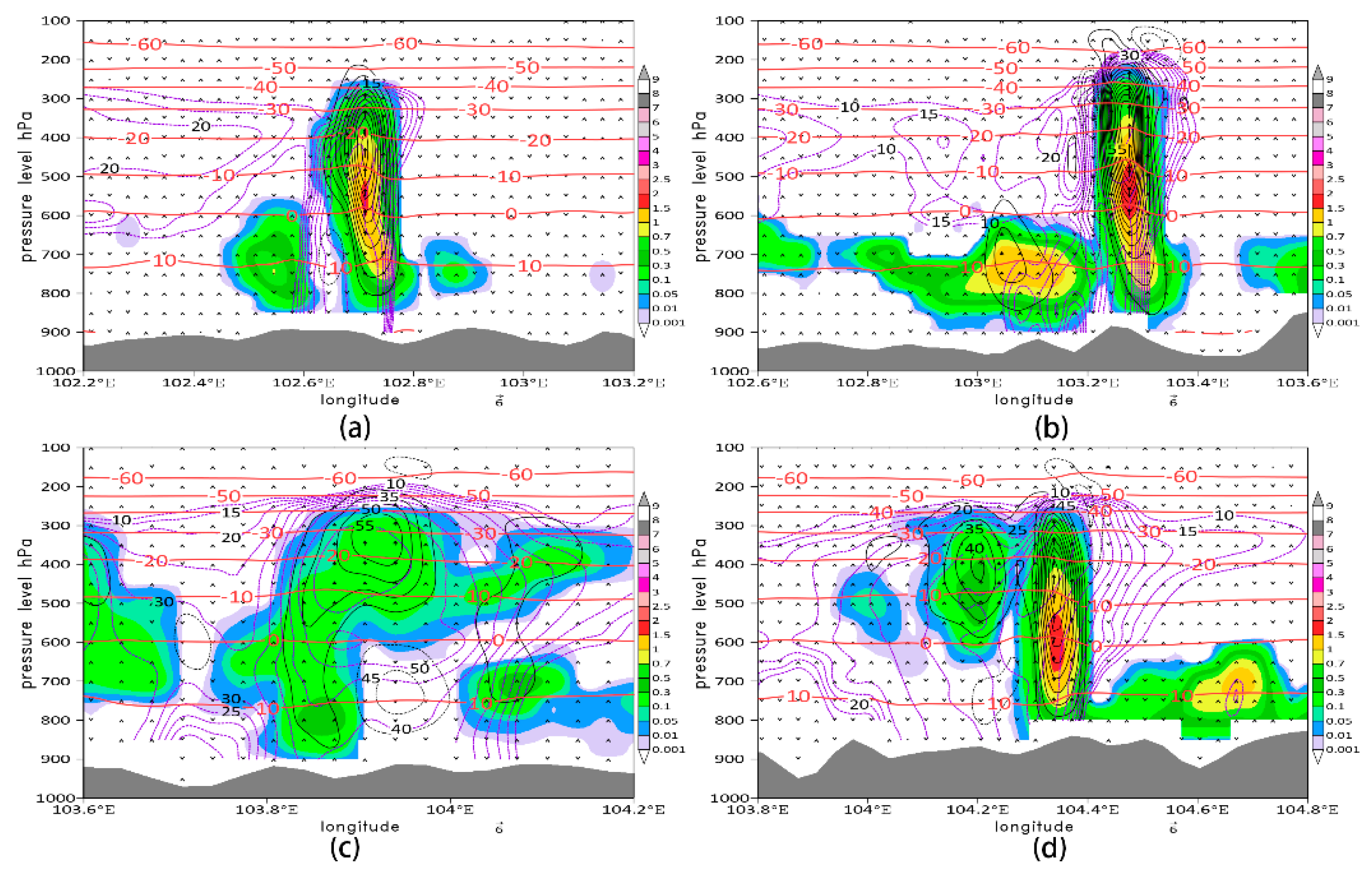
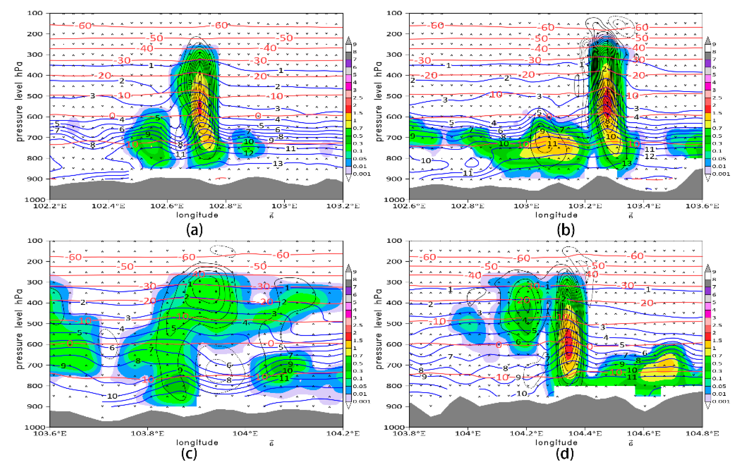
The model can simulate the mesoscale convergence lines formed by the confluence of upper airflow, leading to the formation and development of convective cloud bands. Meanwhile, the convergence of lower-level wind direction or wind speed and upper-level divergence are conducive to the lower-level warm and humid air convergence into the cloud, and the formation of the deep tilted updraft, with the updraft up to 12~15 m·s⁻¹ at the −40~−10 °C layer, leading to the intense development of local convective clouds.

(d)

The formation of hail embryos is closely related to the content of cloud water and snow crystals but has little to do with that of rainwater and ice crystals. The rich and deep cloud water droplets converge and uplift along the deep updraft. The hail embryos firstly grow through the collision-freezing with the supercooled cloud water droplets in the middle-low level, and further increase through the accretion with the snow crystals in the middle-upper level.

However, due to the limitations of the products of the business-as-usual model in the paper, it is impossible to further study how they discern accretion and collision-coalescence processes among different hydrometeors. In the future, we plan to carry out research on hail weather by using the mesoscale cloud-resolving model and the spectral (bin) microphysics cloud model, especially the research of the accretion and collision-coalescence processes among different hydrometeors in the low-latitude plateau area. Also, the WRF-ARW has a version containing hail as a hydrometeor in the microphysical scheme, making it possible to study the time of hail generation and the change of hail size. Next, we will use WRF-ARW to explore the simulation study on the hail weather process.

References

1. Zhang, C.; Zhang, Q.; Wang, Y. Climatology of Hail in China: 1961–2005. J. Appl. Meteorol. Clim. 2008, 47, 795–804. [Google Scholar] [CrossRef]
2. Burcea, S.; Cică, R.; Bojariu, R. Hail Climatology and Trends in Romania: 1961–2014. Mon. Weather Rev. 2016, 144, 4289–4299. [Google Scholar] [CrossRef]
3. Kahraman, A.; Tilev-Tanriover, Ş.; Kadioglu, M.; Schultz, D.M.; Markowski, P.M. Severe Hail Climatology of Turkey. Mon. Weather Rev. 2016, 144, 337–346. [Google Scholar] [CrossRef] [Green Version]
4. Xie, B.; Zhang, Q.; Wang, Y. Trends in hail in China during 1960–2005. Geophys. Res. Lett. 2008, 35, 13801. [Google Scholar] [CrossRef] [Green Version]
5. Huang, Y.; Wang, X.; Pei, J.; Ma, Y. Mesoscale characteristics of a rare severe hailstorm event. Theor. Appl. Clim. 2019, 132, 159–170. [Google Scholar] [CrossRef]
6. Amburn, S.A.; Wolf, P.L. VIL Density as a Hail Indicator. Weather Forecast. 1997, 12, 473–478. [Google Scholar] [CrossRef] [Green Version]
7. Bauer-Messmer, B.; Waldvogel, A. Satellite data based detection and prediction of hail. Atmos. Res. 1997, 43, 217–231. [Google Scholar] [CrossRef]
8. Reynolds, D.W. Observations of Damaging Hailstorms from Geosynchronous Satellite Digital Data. Mon. Weather Rev. 1980, 108, 337–348. [Google Scholar] [CrossRef]
9. Foote, G.B.; Frank, H.W. Case Study of a Hailstorm in Colorado. Part III: Airflow from Triple-Doppler Measurements. J. Atmos. Sci. 1983, 40, 686–707. [Google Scholar] [CrossRef] [Green Version]
10. Guo, X.; Guo, X.L.; Chen, B.J.; He, H.; Ma, X.C.; Tian, P.; Zhang, X. Numerical Simulation on the Formation of Large-size Hailstones. J. Appl. Meteorol. Sci. 2019, 30, 651–664. [Google Scholar]
11. Hopper, J.L.J.; Schumacher, C.; Humes, K.; Funk, A. Drop-Size Distribution Variations Associated with Different Storm Types in Southeast Texas. Atmosphere 2019, 11, 8. [Google Scholar] [CrossRef] [Green Version]
12. Thurai, M.; Steger, S.; Teschl, F.; Schönhuber, M. Analysis of Raindrop Shapes and Scattering Calculations: The Outer Rain Bands of Tropical Depression Nate. Atmosphere 2020, 11, 114. [Google Scholar] [CrossRef] [Green Version]
13. Hong, Y.C. A 3-D Hail Cloud Numerical Seeding Model. Acta Meteor Sin. 1998, 56, 641–653. [Google Scholar]
14. Fovell, R.G.; Tan, P. The Temporal Behavior of Numerically Simulated Multicell-Type Storms. Part II: The Convective Cell Life Cycle and Cell Regeneration. Mon. Weather Rev. 1998, 126, 551–577. [Google Scholar] [CrossRef]
15. Buckley, B.W.; Wang, Y.; Leslie, L.M. The Sydney Hailstorm of April 14, 1999: Synoptic description and numerical simulation. Meteorol. Atmos. Phys. 2001, 76, 167–182. [Google Scholar] [CrossRef]
16. Blair, A.; Metropolis, N.; Von Neumann, J.; Taub, A.H.; Tsingou, M. A Study of a Numerical Solution to a Two-Dimensional Hydrodynamical Problem. Math. Tables Aids Comput. 2006, 13, 145. [Google Scholar] [CrossRef]
17. Wang, X.M.; Zhong, Q.; Han, S.Y. A Numerical Case Study on the Evolution of Hail Cloud and the Three-Dimensional Structure of Supercell. Plateau Meteor. 2009, 28, 352–365. [Google Scholar]
18. Hong, Y.C.; Xiao, H.; Li, H.Y.; Hu, Z.X. Studies on Microphysical Processes in Hail Cloud. Chin. J. Atmos. Sci. 2002, 26, 421–432. (In Chinese) [Google Scholar]
19. Guo, X.L.; Huang, M.Y.; Hong, Y.C.; Xiao, H.; Zhou, L. A Study of Three-Dimensional Hail-Category Hailstorm Model Part I: Model Description and the Mechanism of Hail Recirculation Growth. Chin. J. Atmos. Sci. 2001, 25, 707–720. (In Chinese) [Google Scholar]
20. Guo, X.L.; Huang, M.Y.; Hong, Y.C.; Xiao, H.; Zhou, L. A Study of Three-Dimensional Hail-Category Hailstorm Model Part Ⅱ: Characteristics of Hail-Category Size Distribution. Chin. J. Atmos. Sci. 2001, 25, 856–864. (In Chinese) [Google Scholar]
21. Weisman, M.L.; Skamarock, W.C.; Klemp, J.B. The Resolution Dependence of Explicitly Modeled Convective Systems. Mon. Weather Rev. 1997, 125, 527–548. [Google Scholar] [CrossRef]
22. Kain, J.S. The Kain–Fritsch convective parameterization: An update. J. Appl. Meteor. 2004, 43, 170–181. [Google Scholar] [CrossRef] [Green Version]
23. Skamarock, W.C.; Klemp, J.B.; Dudhia, J.; Gill, D.O.; Barker, D.M.; Duda, M.G.; Huang, X.; Wang, W.; Powers, J.G. A Description of the Advanced Research WRF Version 3; NCAR Tech. Note NCAR/TN-475+STR; National Center for Atmospheric Research: Boulder, CO, USA, 2008; p. 113. [Google Scholar]
24. Adams-Selin, R.D.; Ziegler, C.L. Forecasting Hail Using a One-Dimensional Hail Growth Model within WRF. Mon. Weather Rev. 2016, 144, 4919–4939. [Google Scholar] [CrossRef]
25. Kang, F.Q.; Zhang, Q.; Qu, Y.X.; Ji, L.Z.; Guo, X.L. Simulating Study on Hail Microphysical Process on the Northeastern Side of Qinghai-Xizang Plateau and Its Neighborhood. Plateau Meteor. 2004, 23, 735–742. [Google Scholar]
26. Fu, Y.; Liu, X.L.; Ding, W. A Numerical Simulation Study of a Severe Hail Event and Physical Structure of Hail Cloud. J. Trop. Meteorol. 2016, 32, 546–557. [Google Scholar]
27. Zhang, X.J.; Tao, Y.; Liu, G.Q.; Peng, Y.X. Study on the Evolution of Hailstorm and Its Cloud Physical Characteristics. Meteorol. Mon. 2019, 45, 415–425. [Google Scholar]
28. Zhang, T.F.; Duan, X.; Lu, Y.B.; Hai, Y.S. Circulation background for a severe convective hailstorm weather process in Yunnan and its Doppler radar echo features. Plateau Meteor. 2006, 25, 531–538. [Google Scholar]
29. Tao, Y.; Duan, X.; Duan, C.C.; Duan, W. Change Characteristic of Yunnan Hail. Plateau Meteor. 2011, 30, 1108–1118. [Google Scholar]
30. Zhang, T.F.; Zhang, J.; Zhang, S.D.; Zhu, L. Mesoscale Characteristics and Environmental Conditions of South Trough Squall-Line Hailstorm in Yunnan. Plateau Meteor. 2018, 37, 958–969. [Google Scholar]
31. Lou, X.F. Development and Implementation of a New Explicit Microphysical Scheme and Comparisons of Original Schemes of MM5. Ph.D. Thesis, Peking University, Beijing, China, 2002; 140p. (In Chinese). [Google Scholar]
32. Lou, X.F.; Hu, Z.J.; Wang, P.Y.; Zhou, X.J. Introduction to Microphysical Schemes of Mesoscale Atmospheric Models and Cloud Models. J. Appl. Meteorol. Sci. 2003, 14, 50–59. [Google Scholar]
33. Hu, Z.J.; Yan, C.F. Numerical Simulation of Microphysical Processes in Stratiform Clouds (I)—Microphysical Model. J. Acad. Meteorol. Sci. 1986, 1, 37–52. [Google Scholar]
34. Hu, Z.J.; He, G.F. Numerical Simulation of Microphysical Processes in Cumulonimbus—PART I: Microphysical Model. Acta Meteorol. Sin. 1987, 45, 467–484. [Google Scholar]
35. Gao, W.H.; Zhao, F.S.; Hu, Z.J.; Zhou, Q. Improved CAMS Cloud Microphysics Scheme and Numerical Experient Coupled with WRF. Chin. J. Geophys. 2012, 55, 396–405. (In Chinese) [Google Scholar]
36. Hong, S.-Y.; Noh, Y.; Dudhia, J. A New Vertical Diffusion Package with an Explicit Treatment of Entrainment Processes. Mon. Weather Rev. 2006, 134, 2318–2341. [Google Scholar] [CrossRef] [Green Version]
37. Mlawer, E.J.; Taubman, S.J.; Brown, P.D.; Iacono, M.J.; Clough, S.A. Radiative transfer for inhomogeneous atmospheres: RRTM, a validated correlated-k model for the longwave. J. Geophys. Res. Space Phys. 1997, 102, 16663–16682. [Google Scholar] [CrossRef] [Green Version]
38. Chou, M.D.; Suarez, M.J. An efficient thermal infrared radiation parameterization for use in general circulation models. NASA Tech. Memo. 1994, 10, 85. [Google Scholar]
39. Chou, M.-D.; Suarez, M.J.; Ho, C.-H.; Yan, M.M.-H.; Lee, K.-T. Parameterizations for Cloud Overlapping and Shortwave Single-Scattering Properties for Use in General Circulation and Cloud Ensemble Models. J. Clim. 1998, 11, 202–214. [Google Scholar] [CrossRef]
40. Hu, Z.X.; Li, H.Y.; Xiao, H.; Hong, Y.C.; Huang, M.Y.; Wu, Y.X. Numerical Simulation of Hailstorms and the Characteristics of Accumulation Zone of Supercooled Raindrops. Clim. Environ. Res. 2003, 8, 196–208. [Google Scholar]
41. Hu, Z.X.; Qi, Y.B.; Guo, X.L.; Hong, Y.C. Numerical Simulation of Hail Formation Mechanism in East of the Tibetan Plateau. Clim. Environ. Res. 2007, 12, 37–48. [Google Scholar]
42. Hu, Z.X.; Guo, X.L.; Li, H.Y.; Hong, Y.C. Numerical Simulation of a Hybrid-Type Hailstorm in Munich and the Mechanism of Hail Formation. Chin. J. Atmos. Sci. 2007, 31, 973–986. (In Chinese) [Google Scholar]
43. Sulakvelidze, G.K.; Bibilashviti, N.S.; Lapcheva, V.F. Formation of Precipitation and modification of Hail Processes; The Israel Program for Scientific Translations (I.P.S.T Publisher): Jerusalem, Israel, 1967. [Google Scholar]
Figure 1. (a) Distribution of gale (m s−1, shadowed fields are wind velocity ≥17 m s−1) from 18 March 2019 12:00 UTC to 19 March 2019 12:00 UTC) and counties with hail shots (black triangles represent the 1st hail from 18 March 2019 22:40 UTC to 19 March 2019 02:00 UTC and red triangles represent the 2nd hail from 19 March 2019 08:00 UTC to 10:00 UTC), and (b,c) the real photographs of hail in downtown Jinping County.
Atmosphere 12 00063 g001
Figure 2. (a) 500 hPa geopotential height (dagpm) and wind field (arrow, m s−1, shadowed fields are wind velocity ≥ 12 m s−1), and (b) 700 hPa flow field (streamline) and relative humidity (%, shadowed fields are relative humidity (RH) ≥50%) on 18 March 2019 at 12:00 UTC. Thick solid lines represent south branch trough (SBT), the red curve is the border of Yunnan Province, and the blue triangles represent counties with hail shots.
Atmosphere 12 00063 g002
Figure 3. Plan position indicator (PPI) (0.5° elevation angle) of reflectivity factor (dBz, a,c,e,g) and radial velocity (m s−1, b,d,f,h) at (a,b) 23:40 UTC on 18 March 2019 and at (c,d) 00:45 UTC on 19 March 2019 for 1st hail, and at (e,f) 08:00 UTC and (g,h) 09:00 UTC on 19 March 2019 for 2nd hail.
Atmosphere 12 00063 g003
Figure 4. RHI of reflectivity factor (dBz, a,c) and radial velocity (m s−1, b,d) at (a,b) 00:00 UTC for 1st hail and at (c,d) 09:00 UTC for 2nd hail on 19 March.
Atmosphere 12 00063 g004
Figure 5. Simulation result of reflectivity factor (dBz, color) and wind field (arrow) at 700 hPa for 1st hail at (a) 22:00 UTC and (b) 23:00 UTC on 18 March 2019, and at (c) 00:00 UTC and (d) 01:00 UTC on 19 March 2019.
Atmosphere 12 00063 g005
Figure 6. Simulation result of reflectivity factor (dBz, color) and wind field (arrow) at 700 hPa for 2nd hail at (a) 08:00 UTC and (b) 09:00 UTC on 19 March.
Atmosphere 12 00063 g006
Figure 7. Vertical profile of reflectivity factor (dBz, color), uw wind field (m s−1, streamline) and temperature (°C, thick red contour) of simulation for 1st hail at (a) 22:00UTC and (b) 23:00 UTC on 18 March 2019, and at (c) 00:00 UTC and (d) 01:00 UTC on 19 March 2019.
Atmosphere 12 00063 g007
Figure 8. Vertical profile of reflectivity factor (dBz, color), uw wind field (m s−1,stream line) and temperature (°C, thick red contour) of simulation for 2nd hail at (a) 08:00 UTC and (b) 09:00 UTC on 19 March 2019.
Atmosphere 12 00063 g008
Figure 9. Temporal and height distributions of (a) qc, (b) qs, (c) qr, (d) qi and (e) qg (g·kg−1, black line) from 18 March 2019 21:00 UTC to 19 March 2019 01:00 UTC for 1st hail, thick red solid lines are isotherm.
Atmosphere 12 00063 g009
Figure 10. Temporal-height distributions of (a) qng and (b) qns (kg−1, black line) from 18 March 2019 21:00 UTC to 19 March 2019 01:00 UTC for 1st hail, thick red solid lines are isotherm.
Atmosphere 12 00063 g010
Figure 11. Vertical profile of reflectivity factor (dBz, the purple dashed line), vertical wind velocity and direction (m s−1, the thin black contour and arrow), temperature (°C, the thick red contour), and qc (g·kg−1, color) at (a) 21:00 UTC, (b) 22:00 UTC, and (c) 23:00 UTC on 18 March 2019, and (d) 00:00 UTC on 19 March 2019.
Atmosphere 12 00063 g011
Figure 12. Vertical profile of vertical wind velocity and direction (m s−1, the thin black contour and arrow), temperature (°C, the thick red contour), qc (g·kg−1, color), and qv (g·kg−1, the blue contour) at (a) 21:00 UTC, (b) 22:00 UTC and (c) 23:00 UTC on 18 March, and (d) 00:00 UTC on 19 March.
Atmosphere 12 00063 g012
Publisher’s Note: MDPI stays neutral with regard to jurisdictional claims in published maps and institutional affiliations.