Article

Evaluation and Expected Changes of Summer Precipitation at Convection Permitting Scale with COSMO-CLM over Alpine Space

Fondazione Centro Euro-Mediterraneo sui Cambiamenti Climatici (CMCC), Viale Thomas Alva Edison s.n.c., 81100 Caserta (CE), Italy
*
Author to whom correspondence should be addressed.
Atmosphere 2021, 12(1), 54; https://doi.org/10.3390/atmos12010054
Submission received: 13 November 2020 / Revised: 23 December 2020 / Accepted: 29 December 2020 / Published: 31 December 2020

Abstract

:
There is an ongoing debate in the climate community about the benefits of convection-permitting models that explicitly resolve convection and other thermodynamical processes. An increasing number of studies show improvements in Regional Climate Model (RCM) performances when the grid spacing is increased to 1-km scale. Up until now, such studies have revealed that convection-permitting models confer significant advantages in representing orographic regions, producing high-order statistics, predicting events with small temporal and spatial scales, and representing convective organization. The focus of this work is on the analysis of summer precipitation over the Alpine space. More specifically, the driving data are downscaled using the RCM COSMO-CLM first at an intermediate resolution (12 km) over the European Domain of Coordinated Downscaling Experiment (EURO-CORDEX domain). Then, a further downscaling at 3 km, nested into the previous one, is performed over the Alpine domain to exploit the results over a complex orography context. Experiments of evaluation, historical and far future under the Intergovernmental Panel on Climate Change (IPCC) RCP8.5 scenario have been considered. Indices as mean precipitation, frequency, intensity, and heavy precipitation are employed in daily and hourly analyses. The results, observed from the analysis of 10 year-long simulations, provide preliminary indications, highlighting significant differences of the convection permitting simulations with respect to the driving one, especially at an hourly time scale. Moreover, future projections suggest that the convection permitting simulation refines and enhances the projected patterns, compared with the coarser resolution.

1. Introduction

At present, it is widely recognized that extreme precipitation is becoming more frequent and intense in warmer climates, in response to anthropogenic forcing [1,2]. Extreme precipitation events are the main causes for different hazards (e.g., floods), and play an important role for engineers and hydrologists involved in the update of existing design standards of structures, such as dams, bridges, and sewage systems to potential future changes, as well as for land use planning and socioeconomic purposes [3,4]. Such evidence suggests the need to provide climate information at properly temporal (preferably hourly) and spatial (preferably ~1–3 km) scales, concerning current climate and future projections. In the last decade, several strategies have been deployed to achieve these spatial and temporal scales [5]. Various works provide reports about significant improvements using regional climate models (RCMs) at kilometer-scale resolutions, so-called convection-permitting regional climate models (CP-RCMs), to dynamically downscale general circulation models (GCMs) or RCMs at lower resolutions [6,7,8,9,10,11]. The characteristics defining such a strategy are to explicititly resolve convection by turning off the deep convection parameterizations and run climate simulations at resolutions below 4 km with hourly outputs. The benefits in explicitly resolving convection and other (thermo)dynamical processes are appreciated from the climate community, only with recent computational advances that climate time scales (i.e., decade or longer) are within reach.
As more studies are performed, evidence continues to mount that kilometer-scale modeling brings significant advantages in representing orographic regions, producing high-order statistics, predicting events with small temporal and spatial scales, and representing convective organization [12,13,14,15,16,17]. Specifically, these studies reveal the added value of kilometer-scale modeling in more accurately representing diurnal cycles [6], hourly precipitation intensities, local–regional circulations, seasonal average precipitation, convective downdrafts, and the representation of cold pools [18]. In addition to these direct effects, there are further benefits, e.g., a more accurate representation of interactions with complex topography, urban effects, land-ocean contrasts, and land surface heterogeneities, which play a key role in forcing or triggering convection. Convection-permitting climate simulations allow the study of complex and fine scale aerosol–cloud–precipitation interactions. Positive indirect effects occur on the representation of regional climate, as well as through various feedback mechanisms, such as soil moisture–precipitation and soil moisture/vegetation–temperature and urban effects. Recently, these models have been applied for climate change studies, showing a significant alteration of the climate change signals, with respect to those projected by conventional climate models [8,15,19,20,21].
On this topic, a complex orographic context, such as that of the Alpine area, often affected by heavy precipitation events, which are likely to be significantly impacted in the future, represents a promising hot-spot to investigate the benefits of CP-RCMs for the current climate [6,11,20,22,23] as for future projections [19,24]. The current state of scientific knowledge on CP-RCMs show that they do not necessarily better represent daily mean precipitation [18], but have significantly better sub-daily rainfall characteristics [6] with improved representation of the spatial structure of rainfall and its duration-intensity characteristics [7], the intensity of hourly precipitation extremes [6,18,20], which are typically poorly represented in climate models. Moreover, the study by [9] provides an analysis of the performance of the 10-year long simulation in comparison with its driving one, and the one by [10], a model-intercomparison of CP-RCM simulations.
The main added value of this article is an objective assessment of the summer precipitation over the Alpine space with a proper quantification of uncertainties, supported by statistical analyses and metrics, addressing the impact of model temporal and spatial resolution on the actual values and future scenarios. In other words, the current study aims to contribute to such an open debate, in the climate community, by attempting to complete the following objectives:
(i)
Investigate behaviors and footprints yielded by a convection-parameterizing climate simulation and a convection-resolving one for summer precipitation at daily and hourly scales;
(ii)
Investigate potential changes in summer precipitation regimes, expected for the end of the century, resulting from the ongoing climate change;
(iii)
Prove limitations and benefits returned by a spatial and temporal refinement of CP-RCM.
To address these objectives, this study presents climate simulations run at different spatial scales (~12 km against ~3 km) and that cover different, 10 year-long periods following evaluation, historical, and far future experiments (2000–2009 for evaluation, 1996–2005 for historical, and 2090–2099 and far future experiments). All of the simulations have been integrated with the COSMO-CLM (COnsortium for Small- Scale MOdeling in Climate Mode) model [25]. The choice to run 10 year-long simulations is adopted in some European projects and initiatives (e.g., European Climate Prediction Horizon 2020 project, CORDEX Flagship Pilot Studies on convection) in order to save computational resources, although climate data on 10 year-long periods only provide preliminary indications, and deserve further study on sufficiently long periods (e.g., 30 years-long) to identify climatologic trends.
The paper is organized as follows: Section 2 contains a description of the methodology used in terms of the COSMO-CLM model, the simulations set-up, the observational datasets, and the statistical analysis; in Section 3, results, in terms of daily analysis, hourly analysis, and projections of future precipitation, are presented and discussed. Concluding remarks are provided in Section 4.

2. Methods

2.1. The COSMO-CLM Model

This study relies on the use of the non-hydrostatic limited-area COSMO-CLM model, designed for simulations at resolutions ranging from the meso-𝛽 (horizontal scales in-between 20–200 km) to the meso-𝛾 (horizontal scales in-between 2–20 km) scales. Such a model solves the fully compressible governing equations of fluid dynamics on a structured grid using finite difference methods [26]. Horizontal advection is calculated using a fifth-order upwind scheme. Vertical advection is computed with an implicit Crank–Nicholson scheme [27]. Time integration is performed with a split-explicit third-order Runge–Kutta discretization [28]. Cloud microphysics are represented with a single moment scheme using five hydrometeors (cloud water, rain, ice crystals, snow, and graupel) [29]. The representation of soil moisture is performed using a 10-layer soil model (TERRA_ML) with a new formulation for water runoff dependent on orography [30]. The bulk scheme named “TERRA-URB” [31,32] provides an intrinsic representation of urban physics in the COSMO-CLM model by modifying the input data, soil-vegetation module TERRA-ML, and the land–atmospheric interactions, discerning between urban canopy and natural land cover for each grid cell with a tile approach. The main features of the urban parameterization are: (i) application of the Semi-empirical URban canopY (SURY) parameterization, converting urban canopy parameters containing the three-dimensional urban-canopy information into bulk parameters [33,34], assuming appropriate parameters for albedo, emissivity, heat capacity, and heat conductivity and aerodynamic roughness length; (ii) representation of buildings and pavements on top of the natural soil, enabling a comprehensive representation of the heterogeneous urban environment that consists of impervious surfaces, bare soil, vegetation, water puddles, and snow mantle; (iii) inclusion of the new bare soil evaporation resistance formulation and the vegetation skin temperature parameterization [35].
The radiation scheme is based on a δ-two-stream approach, as described in [36,37]. Turbulent fluxes within the planetary boundary layer are parameterized with a 1.5-order turbulent kinetic energy (TKE)-based scheme [38,39].
The standard parameterization of convection used in the model is based on [40]. The Tiedtke scheme is a mass-flux closure approach used to parameterize modifications to the vertical structure of the atmosphere due to deep, mid-level, and shallow convection. If the convection is explicitly solved, only the shallow convection part of the scheme is active, while for deeper clouds, the scheme is turned off.

2.2. Simulations Set-Up

The present work focuses on climate simulations at different domains and experiments. The domains are presented in Figure 1 and labeled as “EUR-11” and “ALP-3”: the simulations referring to the latter domain are nested into the previous one. The analysis domains of Figure 1 have been obtained discarding the relaxation zone from the computational domain and allowing a sufficient spinup zone (15 and 23 points, respectively) [41]. The setups for each domain are described in the following. Specifically:
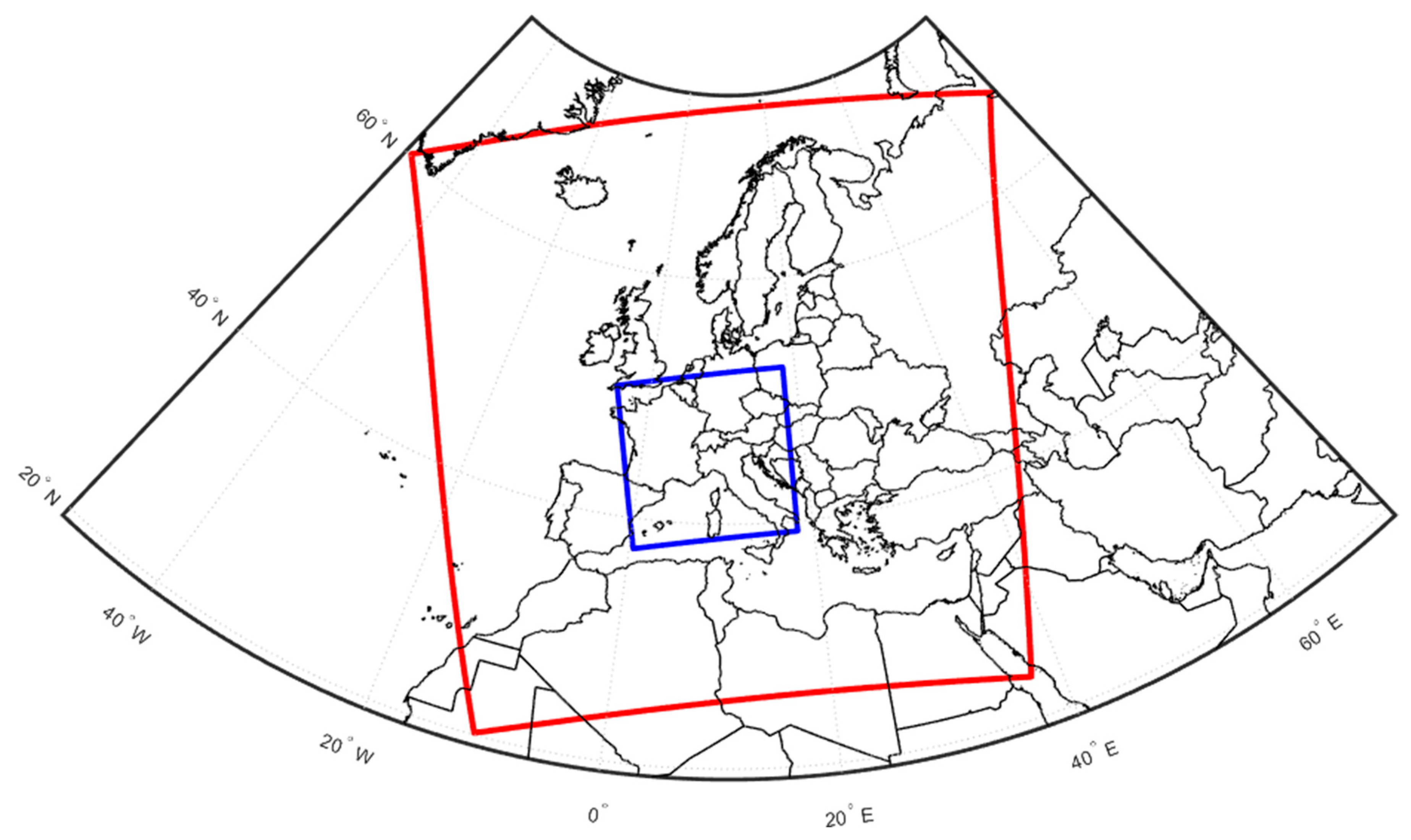
  • EUR-11: it is characterized by a spatial resolution of 0.11° (~12 km) covering the Euro-CORDEX domain (48.50° W–69.86° E; 20.15°–74.01° N) leading to a computational domain with 450 × 438 grid points and 40 vertical levels. The time step for integration is set equal to 75 s. Here the convection is standard parameterized based on the Tiedtke scheme;
  • ALP-3: it is characterized by a spatial resolution of 0.0275° (~3 km) covering an extended Alpine domain from central Italy to northern Germany (4.56° W–18.30° E; 37.50°–52.63° N) leading to a computational domain with 522 × 490 grid points and 50 vertical levels. The time step for integration is set equal to 25 s. The lateral boundary conditions for ALP-3 come from the COSMO-CLM model at 12 km resolution (EUR-11). Here the convection is explicitly solved and TERRA-URB parameterization, for the representation of the urban dynamics, is also used.
Each setup is used to perform 10 year-long simulations considering:
  • Evaluation experiment (2000–2009; 1999 spin-up) initialized with ERA-interim reanalysis [42];
  • Historical experiment (1996–2005; 1995 spin-up) driven by EC Earth general circulation model (GCM) [43];
  • Far future experiment (2090–2099; 2089 spin-up) driven by EC Earth GCM [43] using the IPCC RCP8.5 greenhouse gas scenario [44].
The global datasets used is EC Earth [43] (realization 12) for boundary and lateral conditions. It has a resolution of around 120 km and the update frequency at lateral boundaries is 6h. The datasets used are: GLC2000 [45] for land use, GLOBE for surface altitude and FAO Digital Soil Map of the World for soil types.
Specifically, the evaluation experiments are analyzed with respect to daily and hourly gridded observations to investigate the behaviors and footprints of precipitation patterns and prove the added value and benefits returned by a spatial and temporal refinement. Such an experiment of evaluation is included in [13] for a multi-model study. On the other side, historical and far future experiments are analyzed to evaluate the occurrence of potential change in climate conditions, resulting from the increasing of greenhouse gases at the end of the century.

2.3. Observations

High-resolution observational precipitation datasets (Table 1) available over different regions at daily and sub-daily scales are considered to evaluate the reliability of climate simulations for the evaluation experiment. Specifically:
  • EURO4M-APGD: it is a daily precipitation available at a horizontal resolution of 5 km over the Alpine region from 1971–2008; such a dataset is based on daily rain gauge station data, and is presented in [46];
  • GRIPHO: it is an hourly gridded precipitation dataset, available over Italy at a horizontal resolution of 3 km [47]; such a dataset is based on rain gauge measurements and is available for the period 2001–2016;
  • COMEPHORE: it is an hourly observational dataset with a resolution of 1 km with coverage over metropolitan France [11,48]; such a dataset relies on a combination of rain gauges and radar.
Some insights related to observational gridded datasets of precipitation have to be accounted for [46,47,48,49]: (i) shortcomings associated with these types of datasets, including underestimation of precipitation, especially over mountainous regions due to the sparseness of stations at high elevations, and mask effect problems in areas with high altitude for radar data; (ii) The systematic wind-induced rain gauge under-catch; (iii) wetting and evaporation losses; and (iv) interpolation methods, which systematically induce underestimation of high intensities (smoothing effect) and overestimation of low intensities (moist extension into dry areas).
For the analyses, only the observational periods that overlap with the targeted simulation ones are considered, which are 2000–2008 for EURO4M-APGD data, and 2001–2005 for GRIPHO and COMEPHORE data. The shortfall of observed data is pronounced, especially for hourly precipitation. Anyway, the comparison between the observations and model data is included to report if the characteristics and statistics of precipitation are addressed.

2.4. Climate Indicators and Statistical Tools

The characteristics of precipitation and extremes are investigated at hourly and daily scales for evaluation purposes, considering evaluation experiments with respect to observations, and for assessing the climate change signal by normalizing the difference between far future and historical experiments, with respect to the historical ones.
Table 2 lists the indicators assumed for the analysis at hand. Such a list includes statistical measures, such as mean precipitation, wet day/hour frequency, and wet day/hour intensity, and extreme value analysis, to estimate extreme precipitation events.
Wet day (hour) is defined as a day (hour) with precipitation ≥1 mm/d (≥0.1 mm/h), while the extreme precipitation events are investigated through the amount of daily and hourly precipitation above fixed percentiles computed from all data (wet and dry events), according to [50]. In this study, the 99th percentile is adopted for daily data while the 99.9th percentile for hourly data, chosen to agree with the multi-model studies proposed by [12,13].
All indicators are computed for simulated precipitation over 10-year long periods for the summer season (JJA = June–July–August). Such a period is sufficient for evaluation analysis [51], while, in a rigorous manner, it does not represent a sufficiently long period to identify climatologic trends. Anyway, a 10-year long period could be considered credible to provide preliminary indications about expected future changes, despite the potential impact of the internal variability.
For both evaluation and climate change signal analyses, the indicators are first qualitatively analyzed in terms of spatial distributions through maps. Moreover, some metrics widely adopted for performance evaluation have been assessed. In order to show a fair comparison between models, before the computation of metrics, the simulations are referred to a common domain and interpolated on a common grid (EUR-11), using a conservative remapping. The root mean square error (RMSE) is assessed as:
R M S E = 1 N i = 1 N ( S i O i ) 2
where S and O refer to observation and model, respectively. The standard deviation (STD) of simulated and observed fields is also calculated to highlight spatial variability.
Then, a more focus statistical analysis is performed, considering the spatial cumulative distribution function (CDF) and probability density function (PDF) for evaluation analysis, and the “Whiskers” box plots, [52], for climate change signal analysis, where the cumulative probability is defined as the probability that an event with rainfall x is equal to or greater than F(x). Some authors [53,54,55,56] use distribution functions (as the gamma distribution) to model the cumulative distribution function of precipitation. In this study, we do not use any distribution function, thus the empirical CDFs are proposed to keep as detailed a comparison as possible. The same choice is adopted for PDFs. In order to test the goodness-of-fit statistics, the Anderson–Darling test and the distribution added value are assessed.
The two-sample Anderson–Darling test [57] is used under the null hypothesis that compared samples are drawn from the same population against the alternative hypothesis (that they belong to two populations with different CDFs), with a user-defined level of significance α, usually set to 5%. It is a nonparametric test; thus, it does not require any initial assumption about the distributions to be compared, but it is known to be robust and effective in accounting for both the tails and the central part of the distribution [3]. The analyzed metrics from the two-sample Anderson–Darling test is the standardized Anderson–Darling rank statistic (ADK). High values of ADKs imply that the test fails to reject the null hypothesis and the compared distributions have different CDFs; low values of ADKs imply that the test provides the rejection of the null hypothesis and the compared distributions have similar CDFs.
The distribution added value (DAV) [58] gives the percentage of added value gained or lost by the use of high resolution. Equation (2) measures how well a given high-resolution (Shr) simulation (with respect to a particular observational dataset) compares with a lower resolution (Slr), regarding the same reference dataset (O).
D A V = i = 1 N m i n ( S h r i , O i ) i = 1 N m i n ( S l r i , O i ) i = 1 N m i n ( S l r i , O i )
Regarding the “Whiskers” box plots, it is proposed to synthetically look for differences in the spatial distributions: the central mark indicates the median, and the bottom and top edges of the box indicate the 25th and 75th percentiles, respectively. The expected climate change, addressed by the box plots and maps, is also supported by the metric of the areal mean change (AMC). AMC represents the average change over the plotted area in percentage and it is labeled on the relative maps.

3. Results

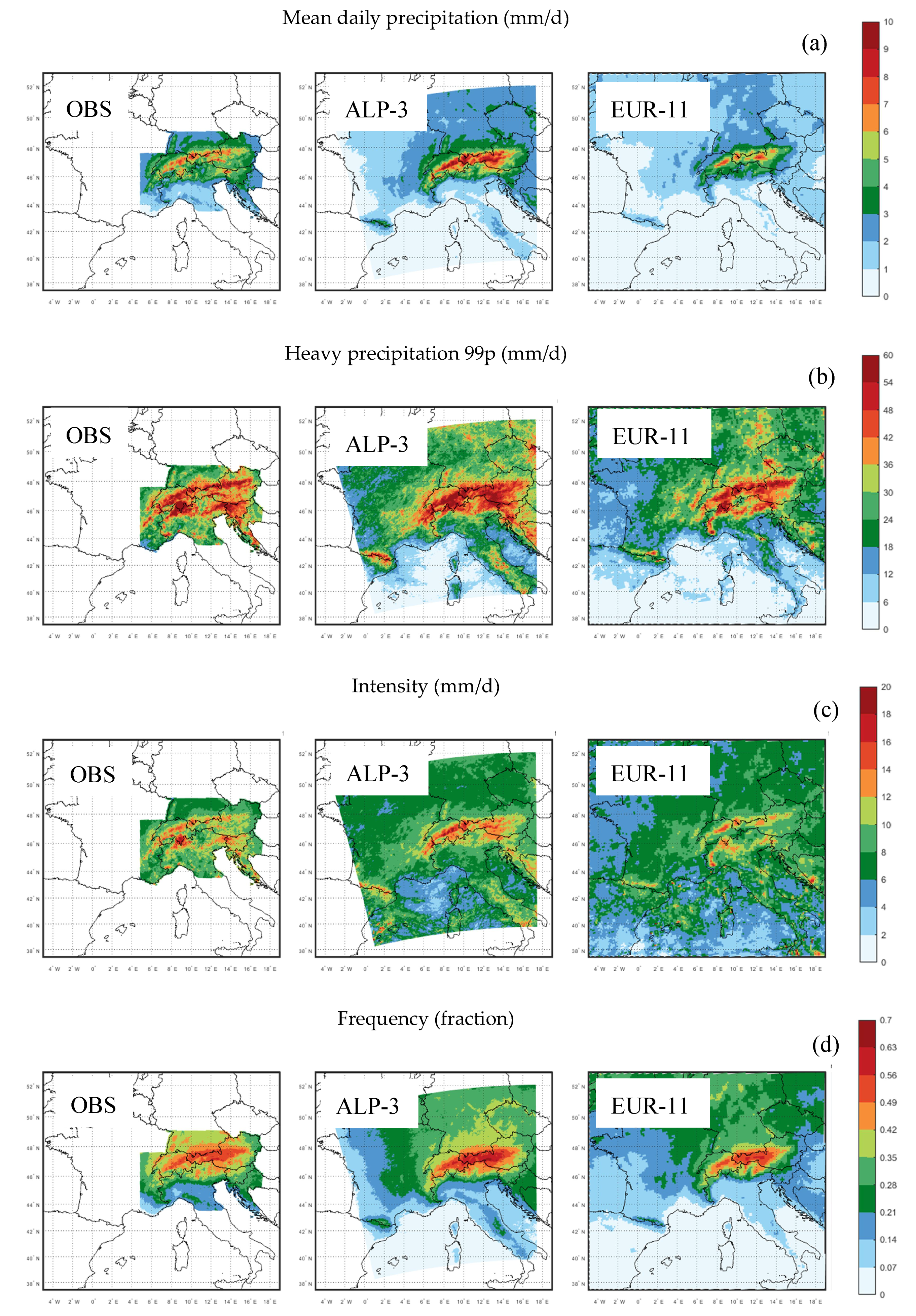
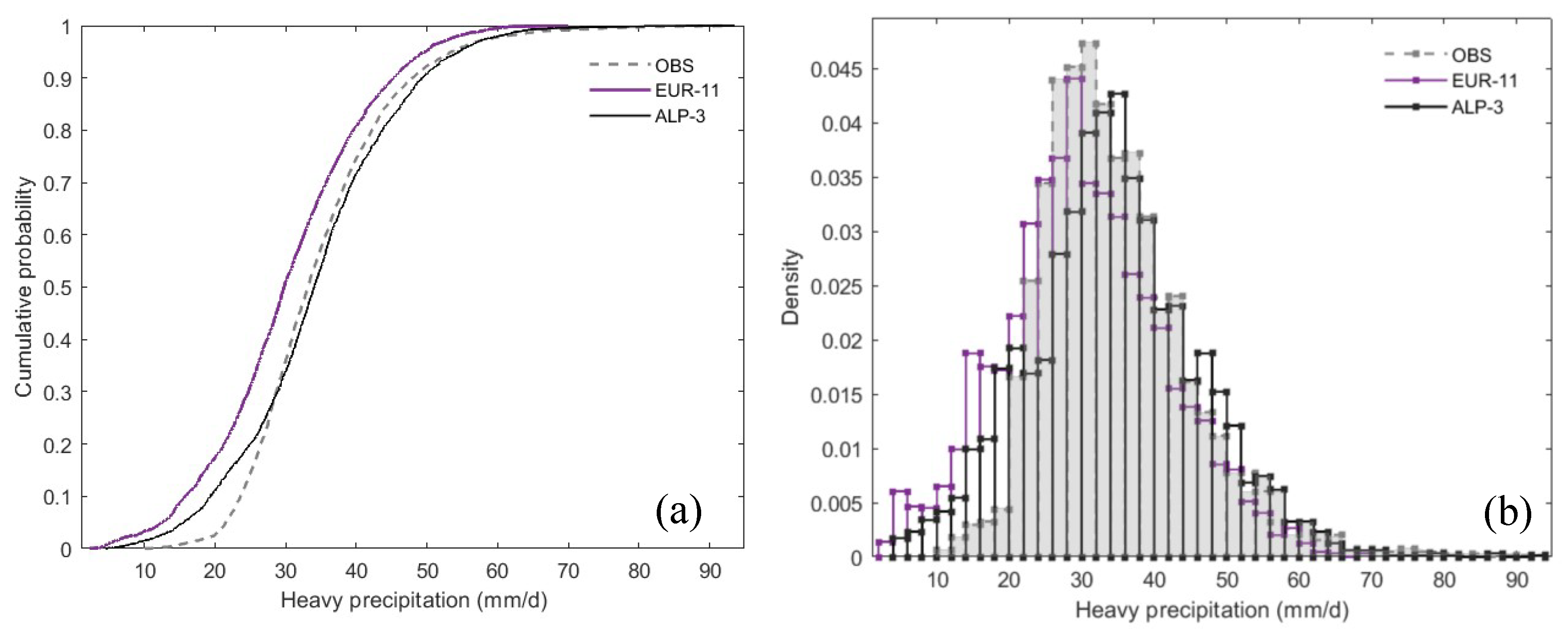
3.1. Precipitation Evaluation at Daily Scale (2000–2009)

Figure 2 compares the spatial distributions at the daily scale of mean precipitation (Figure 2a), heavy precipitation (Figure 2b), frequency (Figure 2c), and intensity (Figure 2d), derived from the evaluation experiments ALP-3 and EUR-11 over summer 2000–2009, with the corresponding plots carried out assuming the dataset EURO4M-APGD over summer 2000–2008 as reference observations. Summer season is characterized by precipitation focusing on regions of high orography. Both simulations ALP-3 and EUR-11 capture the spatial patterns of mean daily precipitation, intensity, frequency, and heavy precipitation quite well, compared to the observations, as confirmed by the metrics RMSE and STD in Table 3.
Some overestimations are present in mean daily precipitation over Alps, especially in ALP-3 results (Figure 2a). Such findings are in agreement with [10]. This is most likely inherited from the overestimation of wet day frequency (Figure 2d) occurring anyway for both simulations, and related to shortcomings of the observational data set. The main differences appear between the ALP-3 and coarse-resolution EUR-11 considering the other indicators. The coarser resolution model EUR-11 exhibits a tendency to underestimate precipitation intensity (Figure 2c) and heavy precipitation (Figure 2b) with respect to observations. The weaker intensity of precipitation and higher wet day frequency indicates persistent light rain, which is consistent with previous studies focusing on evaluation experiments [6,8]. The ALP-3 simulation performs well the heavy precipitation (Figure 2b), although slight overestimations indicate that some problems in initiating small-scale convective summer precipitation still persist over orography.
The comparison addressed by the maps of Figure 2 is complemented by statistically comparing the spatial CDFs and PDFs. In this perspective, the heavy precipitation 99p, calculated in summer over the period 2000–2008 from daily observations, calculated in summer over the period 2000–2009 from ALP-3 and EUR-11 models and plotted in Figure 2, is statistically analyzed to look for any possible differences in the probability distributions, with respect to observations. To make the data comparable, the ALP-3 and EUR-11 simulations refer to a common domain (the one of the EURO4M-APGD dataset) and are regridded to the EUR-11 grid [8,10,17].
Figure 3a presents the empirical CDFs of heavy precipitation 99p, assessed from observations (EURO4M-APGD), ALP-3, and EUR-11 simulations. For ease of interpretation, these functions are differentiated to obtain the corresponding PDFs in Figure 3b. Both climate simulations fit well the observed statistical distribution. The ALP-3 distribution reveals an excellent agreement with observation, with a CDF much closer to observation than the EUR-11 one. The shift of EUR-11 distribution toward low values of heavy precipitation confirms the tendency to underestimations of such distribution compared with the one of observations. These aspects are also highlighted from the comparison by maps of Figure 2. In Table 4, ADKs indicate that the CDF of ALP-3 is more similar to observations than EUR-11, and DAV highlights that the added value gained by the use of high resolution is 3.14%.

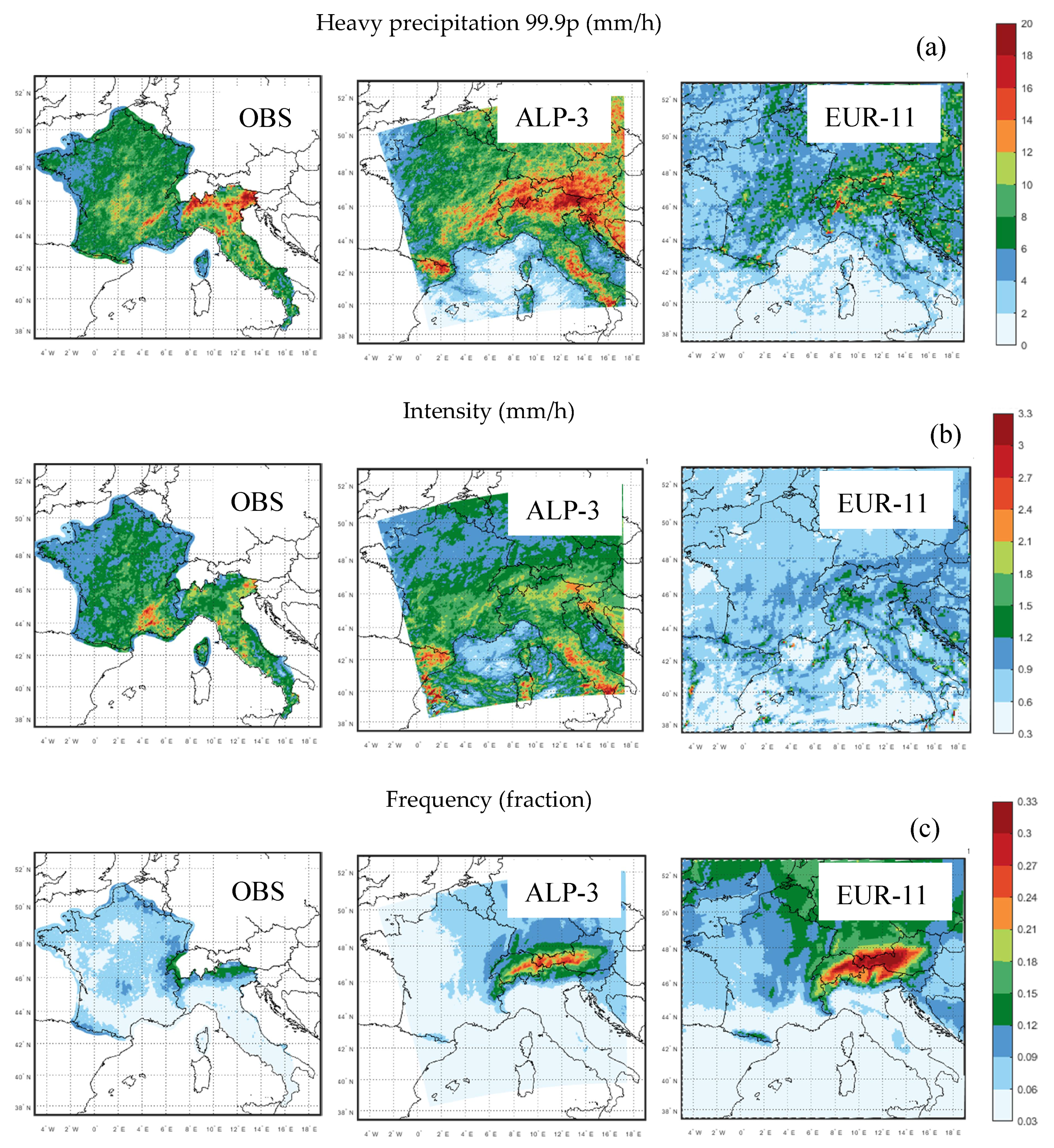
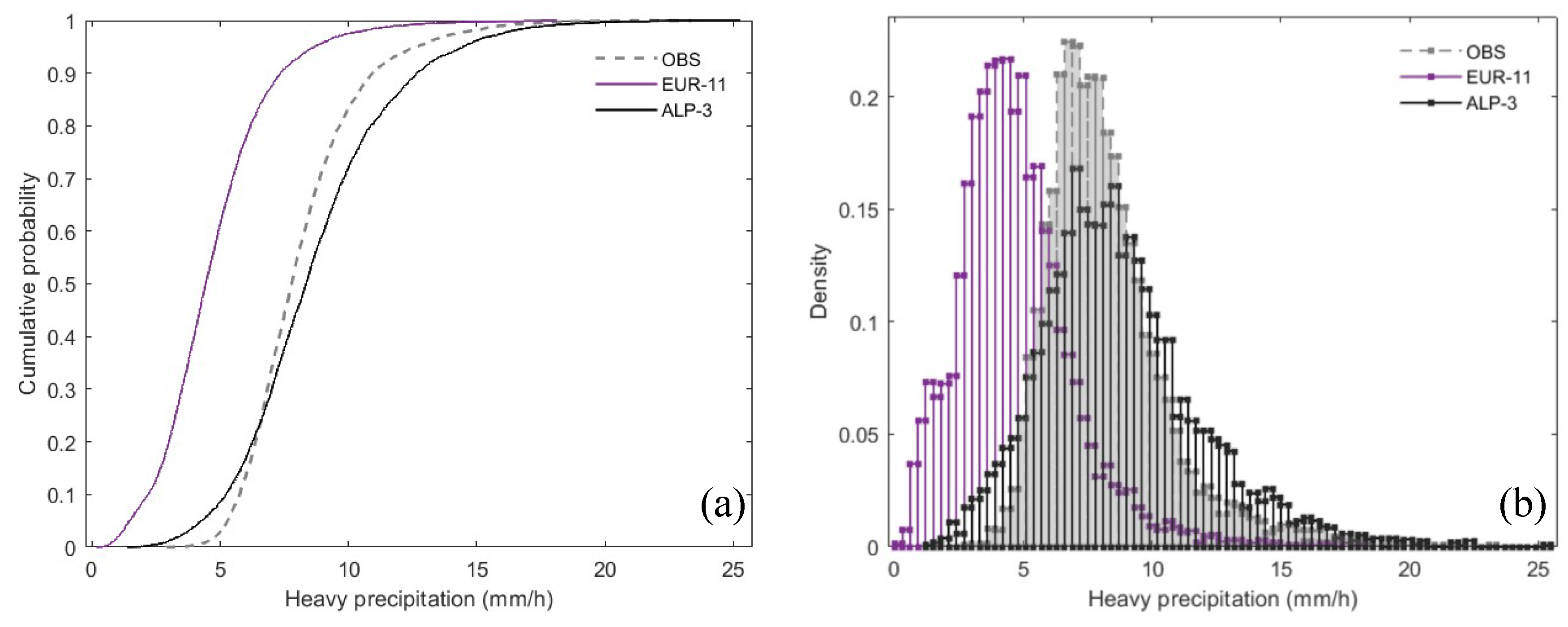
3.2. Precipitation Evaluation at Hourly Scale (2001–2005)

Figure 4 compares the spatial distributions at an hourly scale of heavy precipitation (Figure 4a), frequency (Figure 4b), and intensity (Figure 4c), derived from the evaluation experiments ALP-3 and EUR-11, with respect to the corresponding plots carried out, assuming the gridded datasets at sub-daily resolution (GRIPHO and COMPHORE) as reference observations. Due to the availability of hourly datasets, the simulation results plotted in Figure 4 are over the common period 2001–2005, shared by both evaluation experiments (i.e., 2000–2009) and sub-daily observation datasets (i.e., 1997–2005 for COMPHORE and 2001–2016 for GRIPHO). The differences between simulations ALP-3 and EUR-11 highlighted for daily analyses are further pronounced for hourly precipitation. ALP-3 tends to produce more intense precipitation than its driving coarse resolution model EUR-11 (Figure 4b). Thus, the coarse resolution RCM simulation underestimates heavy precipitation over high orography and lower ground (Figure 4a). Moreover, EUR-11 largely overestimates the wet hour frequency (Figure 4c), especially over mountains, and intensity is strongly underestimated. In other words, the analysis highlights that the EUR-11 provides too light but very frequent precipitation compared to the observations, confirming the results of previous studies [7,9]. The ALP-3 reduces such differences, returning higher intensity and lower frequency of precipitation much closer to the observations than EUR-11. In the sake of clarity, it is worth it to note that the available observations exclude much of the central and eastern mountainous areas of the Alps, and the comparison with observations is allowed over France and part of Italy (as returned by the metrics in Table 5).
This analysis gives indication on the differences between CP-RCM and RCM and on the improvements of the former with respect to the latter, particularly for the hourly-scale analyses and localized over mountains.
As in the case of daily analyses, the qualitative comparison addressed by the maps of Figure 4 is complemented by statistically comparing the spatial cumulative distribution function (CDF) and probability density function (PDF). The heavy precipitation 99.9p, calculated in the summer from hourly observations, ALP-3 and EUR-11 models are statistically analyzed in Figure 5. To make the data comparable, the ALP-3 and EUR-11 simulations refer to a common domain (observations) and are regridded to the EUR-11 grid [8,10,17]. Figure 5a presents the empirical CDFs of heavy precipitation 99.9p, assessed in summer over the period 2001–2005 from observations (GRIPHO and COMPHORE), ALP-3, and EUR-11 simulations.
For ease of interpretation, these functions are differentiated to obtain the corresponding PDFs in Figure 5b. The differences between ALP-3 and EUR-11 simulations highlighted from the maps of Figure 4 are also visible in Figure 5. The ALP-3 distribution shows a very good agreement with the observed statistical distribution, except for slight underestimations for values of heavy precipitation 99.9p lower than 6 mm/h and overestimations for values of heavy precipitation 99.9p higher than 6 mm/h. In any case, the mean value of heavy precipitation 99.9p for ALP-3 distribution (8.2 mm/h) is similar to observations (8.3 mm/h), as well as the shapes of both distributions. This is due to a sort of compensation effect of CP-RCMs, in which intense values are overrepresented and medium events underrepresented. The shift of EUR-11 distribution toward low values of heavy precipitation 99.9p confirms the underestimations of such distribution compared with the one of observations. Moreover, the mean value of heavy precipitation 99.9p for EUR-11 distribution (5.3 mm/h) differs of 3 mm/h from observations (8.3 mm/h), and the whole distribution of data is shifted toward low values of heavy precipitation 99.9p. These aspects are also highlighted from the comparison by maps in Figure 4, where underestimations of heavy precipitation 99.9p from EUR-11 simulation are also assessed. In Table 6, ADKs indicate that the CDF of ALP-3 is more similar to observations than the one of EUR-11, and DAV highlights that the added value gained by the use of high resolution is 129.5%. It is worth noticing how, at hourly time-scale, strong differences between EUR-11 and ALP-3 results emerge.

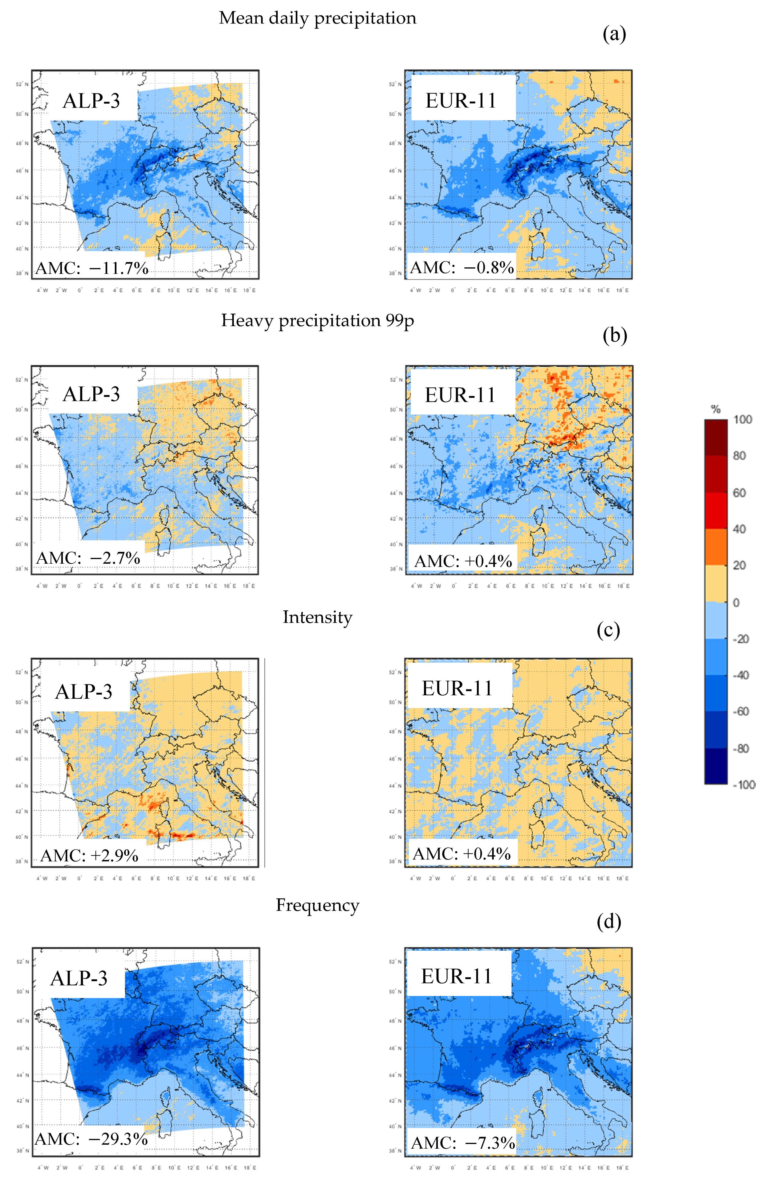
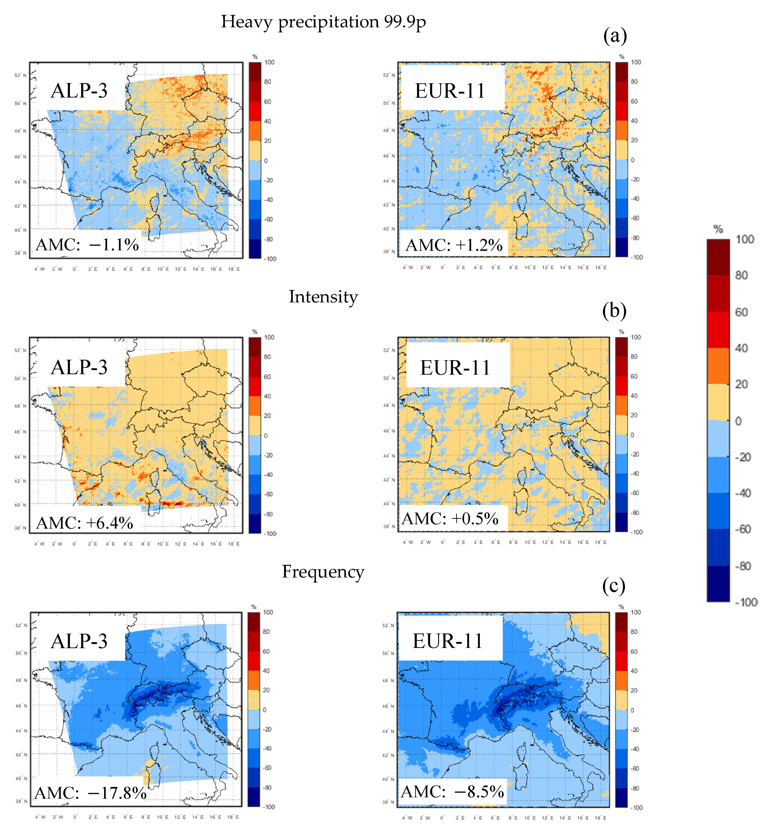
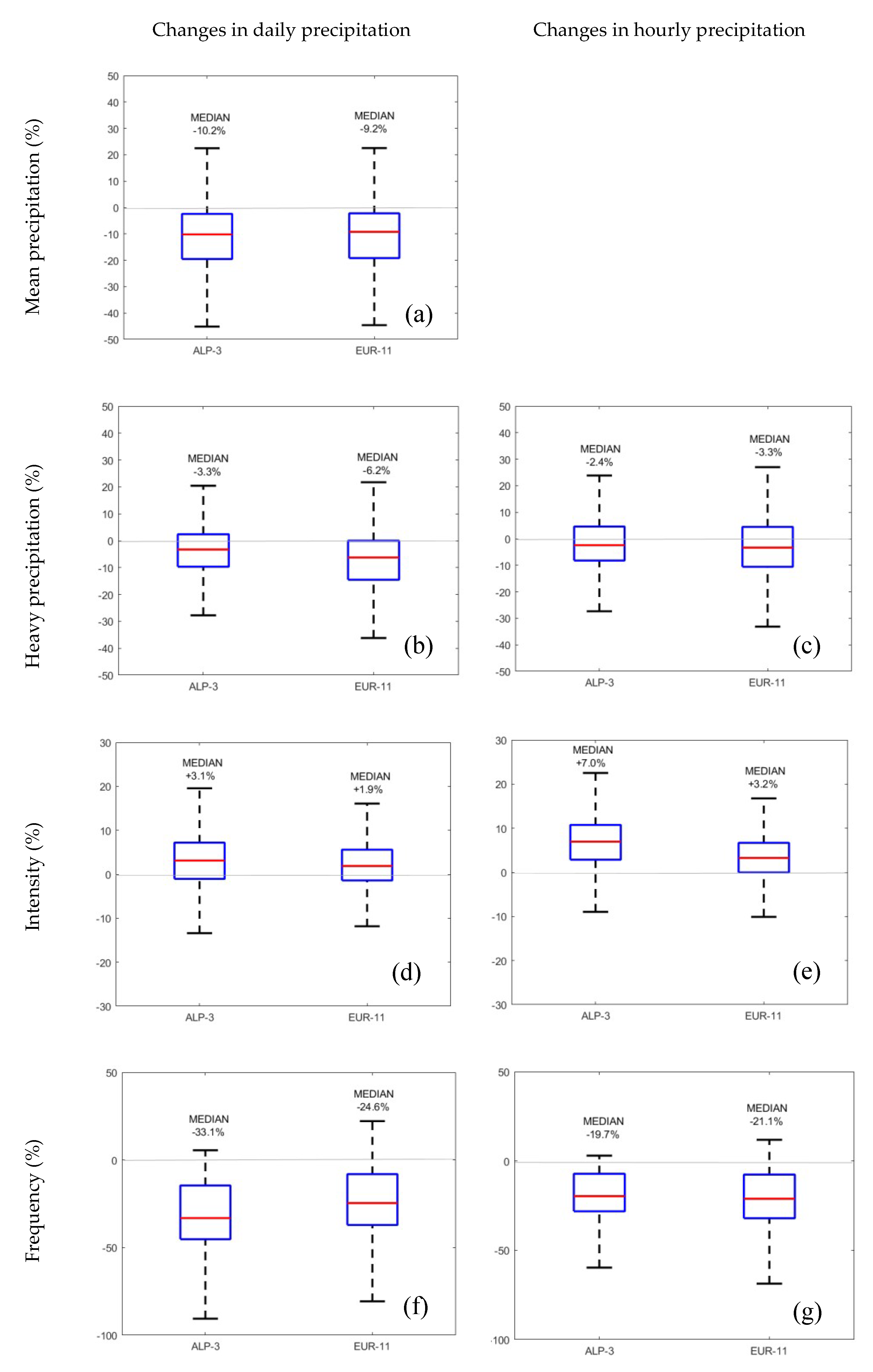
3.3. Future Precipitation Projections (2090–2099 vs. 1996–2005)

The projected changes in summer precipitation are proposed in this section. Figure 6 and Figure 7 plot the changes of mean precipitation (Figure 6a), heavy precipitation (Figure 6b and Figure 7a), frequency (Figure 6c and Figure 7b), and intensity (Figure 6d and Figure 7c) carried out at daily and hourly scale, respectively. In detail, the climate change signals are derived from 10 year-long simulations conducted with ALP-3 and EUR-11 models, as difference between scenario (2090–2099) and historical simulation (1996–2005), normalized by the historical one (1996–2005).
The analyses return a potential decrease in mean precipitation (Figure 6a), which is associated with a decrease in the frequency of daily (Figure 6d) and hourly (Figure 7c) precipitation (as exploited by the AMC). Such a decrease (Figure 6a) is much stronger over the Alps chain. The intensity of daily (Figure 6c) and hourly (Figure 7b) precipitation generally increases, although some areas are slightly in contrast (e.g., a bit of a stronger increase of daily intensity occurs over the north Mediterranean Sea than that of hourly precipitation, and a stronger decrease of daily intensity occurs over France than that of hourly precipitation). Heavy precipitation (Figure 7a) exhibits localized intensification over the eastern Alps and the northern part of the domain, in agreement with [50], visible especially at the hourly scale, and a pronounced drying over the southern part, although the AMC exploits a slight decrease in the areal mean change for ALP-3 and slight increase in EUR-11.
The comparison addressed by the maps in Figure 6 and Figure 7 is complemented by means of the “Whisker” box plots proposed in Figure 8, related to daily and hourly changes of precipitation resulting from both CP-RCM (ALP-3) and RCM (EUR-11) simulations. Both simulations highlight a decrease in projected daily mean precipitation (Figure 8a). The box plots related to the changes of daily heavy precipitation (Figure 8b) for both simulations highlight a decrease, slightly larger in EUR-11 than ALP-3, as for the box plots related to the changes of hourly heavy precipitation (Figure 8c). For the changes of daily intensity (Figure 8d), both simulations highlight an increase (median value of +3.1% for ALP-3 and +1.9% for EUR-11). The box plot related to the changes of hourly intensity (Figure 8e) of ALP-3 shows a median value of +7.0% and EUR-11 has a median value +3.2%. Both simulations highlight a decrease (Figure 8f) in projected daily frequency (larger in ALP-3 than EUR-11, with median values of −33.1% and −24.6%, respectively) and in (Figure 8g) projected hourly frequency (larger in ALP-3 than EUR-11, with median values of −19.7% and −21.1%, respectively).
The projected future change of summer precipitation from the end of century, with respect to the historical period, is then characterized as: (i) a decrease in projected daily mean precipitation; (ii) a general decrease of daily and hourly heavy precipitation with localized intensification over the eastern Alps and the northern part of the domain; (iii) an increase of daily and hourly intensity; and (iv) a reduction in daily and hourly frequency. The differences between the CP-RCM (ALP-3) and RCM (EUR-11) simulations are not so large for both median values and data distributions for almost all indicators, yielding a coherent change projected for summer precipitations.

4. Discussion and Conclusions

In this paper, the summer precipitation over complex orography as the Alpine area was investigated through convection-permitting simulations at a horizontal resolution of ~3 km (ALP-3), and parameterized ones at a horizontal resolution of ~12 km (EUR-11), performed with the COSMO-CLM model. The climate simulations are presented, referring to evaluation (2000–2009), historical (1996–2005), and far future (2090–2099) experiments with RCP8.5 greenhouse gas scenario. The mean, heavy precipitation, frequency, and intensity of summer precipitation are assessed at daily and hourly timescales. Climate data on 10 year-long periods provide only preliminary indications on changes and climatologic trends, especially for extreme patterns having rare occurrences. However, there are current limitations existing on computation resources: they do not perform longer simulation periods, especially on large domains, as the one investigated in this paper.
In the first part of this paper, summer precipitation patterns at daily and hourly scales are investigated, considering evaluation experiments. The comparison among the convection-resolving models, driving convection-parameterizing model, and observations is addressed at a daily scale over the period 2000–2009 and at an hourly scale over the period 2001–2005. Such a comparison reveals that both models capture quite well the spatial patterns of daily precipitation, with high intensity and frequency over high elevations for all analyzed indices. The EUR-11 model tends to underestimate the precipitation intensity and the heavy precipitation, while the ALP-3 model performs better than EUR-11 simulation and the heavy precipitation. Moreover, the heavy precipitation events in ALP-3 are overestimated, in agreement with [10]. The main improvements of ALP-3 are reported for sub-daily precipitation. The ALP-3 model appears to properly reproduce the intensity of precipitation, which is closer to the observed one, while the EUR-11 model tends to underestimate intensity. EUR-11 simulation underestimates heavy precipitation over high orography and lower ground, and largely overestimates the wet hour frequency, while the ALP-3 reduces such differences against observed data. Such findings are also corroborated by statistical analyses of heavy precipitations, resulting in no large differences emerging, in terms of cumulative distribution and probability density functions of ALP-3 and EUR-11 models at daily timescales, although a shift of EUR-11 distribution, compared with observations, toward low values of heavy precipitation, occurs. Such a shift is pronounced at an hourly time-scale with a notable translation of EUR-11 distribution toward low values of heavy precipitation. The results are consistent with previous studies [6,7,18] and multi-model studies [13].
In the second part of this work, potential changes in the summer precipitation regime projected at the end of the century against the historical period are presented. The analysis reveals decreases in mean summer precipitation, especially over topography, and is consistent with conventional climate models [59]. Moreover, the heavy summer precipitation generally decreases, but with localized intensification over the eastern Alps and the northern part of the domain. The decrease in mean and heavy summer precipitation is associated with frequency reductions of small and intermediate precipitation events. Therefore, on daily and hourly time scales, precipitation is projected to become less frequent and more intense. The results are consistent with previous studies [19] and multi-model studies [12]. Both models, ALP-3 and EUR-11, show coherent and consistent changes for daily and hourly precipitation indicators. These remarkable behaviors, observed from the analysis of 10 year-long simulations, provide preliminary indications about the expected changes in future summer precipitation, and deserve further study, employing simulations performed on sufficiently long periods (e.g., 30 years-long) to identify climatologic trends.
Finally, this work aims to contribute to the scientific activities in the climate community by showing the limitations and benefits of running CP–RCMs. On the one hand, the climate change projections show very little difference between EUR-11 and ALP-3, raising the question as to whether the additional computational cost is justified. On the other, the improvements of high-resolution simulations in spatial representation, heavy precipitation, frequency, and intensity of precipitation, are pronounced, compared to coarser resolution counterparts, especially at a sub-daily scale. Moreover, the overestimation of intense events in CP-RCMs, returned by this study, is a well-known issue [10]. Although the climate projections of precipitation are similar between resolutions, the better performance of the ALP-3 model in the evaluation experiment increases the confidence in the CP-RCM projections, particularly for hourly precipitation. Such findings are also supported by the significant difference in the DAV scores proposed in this study, where daily heavy precipitations seems to be, basically, nothing, whereas for hourly, reveals a large improvement. Further studies are needed to understand the actual benefits of CP-RCMs, and if they are due to a better resolution of topography or to the explicit simulation of convection. The proposed results, supported by an ad-hoc quantification of the uncertainties, show that convection-resolving climate models are attractive tools to investigate precipitation climate and its sensitivity to climate change, especially over a hot-spot area (Alpine space) affected by complex precipitation regimes, for current climate and future projections.

Author Contributions

Methodology, all authors; software analysis, M.A. and M.R.; data curation, M.A.; writing—original draft preparation, M.A.; writing—review and editing, M.A., A.R., M.R. and P.M.; Visualization, M.R. and A.R.; Supervision, P.M. All authors have read and agreed to the published version of the manuscript.

Funding

This research received no external funding.

Data Availability Statement

Data and methods used in the research have been presented in sufficient detail in the paper.

Acknowledgments

The authors deeply thank the European Climate Prediction system—Horizon 2020 project (https://www.eucp-project.eu/) and the WCRP-CORDEX-FPS on Convective phenomena at high resolution over Europe and the Mediterranean [FPSCONV-ALP-3]. The experiments have been performed using the COSMO model in CLimate Mode (COSMO-CLM). COSMO-CLM is the community model of the German regional climate re-search jointly further developed by the CLM-Community. The authors acknowledge the members of the community for their common efforts to envelop the model and to find right setups. The authors would like to thank MeteoSwiss, for providing us with observational data set EURO4M-APGD. The authors are also grateful to Météo-France for providing the access to COMPHORE data and to Emanuela Pichelli and Erika Coppola from UNESCO ICTP for allowing access to the Italian database of precipitation GRIPHO.

Conflicts of Interest

The authors declare no conflict of interest.

References

  1. IPCC. Summary for policy makers. In Climate Change 2013: The Physical Science Basis. Contribution of Working Group I to the Fifth Assessment Report of the Intergovernmental Panel on Climate Change; Stocker, T.F., Qin, D., Plattner, G.-K., Tignor, M., Allen, S.K., Boschung, J., Nauels, A., Xia, Y., Bex, V., Midgley, P.M., Eds.; Cambridge University Press: Cambridge, UK; New York, NY, USA, 2013. [Google Scholar]
  2. Allen, M.R.; Ingram, W. Constraints on future changes in climate and the hydrologic cycle. Nature 2002, 419, 224–232. [Google Scholar] [CrossRef] [PubMed]
  3. Padulano, R.; Reder, A.; Rianna, G. An ensemble approach for the analysis of extreme rainfall under climate change in Naples (Italy). Hydrol. Process. 2019, 33, 2020–2036. [Google Scholar] [CrossRef]
  4. Rianna, G.; Reder, A.; Pagano, L.; Mercogliano, P. Assessing future variations in landslide occurrence due to climate changes: Insights from an Italian test case. CNRIG 2019 Geotech. Res. Land Prot. Dev. 2020, 255–264. [Google Scholar] [CrossRef]
  5. Maraun, D.; Widmann, M. Statistical Downscaling and Bias Correction for Climate Research; Cambridge University Press: Cambridge, UK, 2018. [Google Scholar]
  6. Ban, N.; Schmidli, J.; Schär, C. Evaluation of the new convective-resolving regional climate modelling approach in decade-long simulations. J. Geophys. Res. Atmos. 2014, 119, 7889–7907. [Google Scholar] [CrossRef]
  7. Kendon, E.J.; Roberts, N.M.; Senior, C.A.; Roberts, M.J. Realism of rainfall in a very high-resolution regional climate model. J. Clim. 2012, 25, 5791. [Google Scholar] [CrossRef]
  8. Kendon, E.J.; Roberts, N.M.; Fowler, H.J.; Roberts, M.J.; Chan, S.C.; Senior, C.A. Heavier summer downpours with climate change revealed by weather forecast resolution model. Nat. Clim. Chang. 2014, 4, 570–576. [Google Scholar] [CrossRef] [Green Version]
  9. Leutwyler, D.; Luthi, D.; Ban, N.; Fuhrer, O.; Schar, C. Evaluation of the convection-resolving climate modeling approach on continental scales. J. Geophys. Res. Atmos. 2017, 122, 5237–5258. [Google Scholar] [CrossRef]
  10. Berthou, S.; Kendon, E.J.; Chan, S.C.; Ban, N.; Leutwyler, D.; Schär, C.; Fosser, G. Pan-European climate at convection-permitting scale: A model intercomparison study. Clim. Dyn. 2018, 5, 1–25. [Google Scholar] [CrossRef] [Green Version]
  11. Fumiere, Q.; Deque, M.; Nuissier, O.; Somot, S.; Alias, A.; Caillaud, C.; Laurantin, O.; Seity, Y. Extreme rainfall in mediterranean France during the fall: Added value of the CNRM-AROME Convection- permitting regional climate model. Clim. Dyn. 2019. [Google Scholar] [CrossRef] [Green Version]
  12. Pichelli, E.; Coppola, E.; Ban, N.; Giorgi, F.; Stocchi, P.; Antoinette, A.; Danijel, B.; Segolene, B.; Cecile, C.; Rita, M.C. Precipitation projections of the first multi-model ensemble of regional climate simulations at convection permitting scale. EGU Gen. Assem. 2020. [Google Scholar] [CrossRef]
  13. Ban, N.; Brisson, E.; Caillaud, C.; Coppola, E.; Pichelli, E.; Sobolowski, S.; Adinolfi, M.; Ahrens, B.; Alias, A.; Anders, I.; et al. The first multi-model ensemble of regional climate simulations at kilometer-scale resolution, Part I: Evaluation of precipitation. EGU Gen. Assem. 2020. [Google Scholar] [CrossRef]
  14. White, B.A.; Buchanan, A.M.; Birch, C.E.; Stier, P.; Pearson, K.J. Quantifying the effects of horizontal grid length and parameterized convection on the degree of convective organization using a metric of the potential for convective interaction. J. Atmos. Sci. 2018, 75, 425–450. [Google Scholar] [CrossRef] [Green Version]
  15. Kendon, E.J.; Ban, N.; Roberts, N.M.; Fowler, H.J.; Roberts, M.J.; Chan, S.C.; Evans, J.P.; Fosser, G.; Wilkinson, J.M. Do convection-permitting regional climate models improve projections of future precipitation change? Bull. Am. Meteorol. Soc. 2017, 98, 79–93. [Google Scholar] [CrossRef]
  16. Prein, A.F.; Langhans, W.; Fosser, G.; Ferrone, A.; Ban, N.; Goergen, K.; Keller, M.; Tölle, M.; Gutjahr, O.; Feser, F.; et al. A review on regional convection-permitting climate modeling: Demonstrations, prospects, and challenges. Rev. Geophys. 2015, 53, 323–361. [Google Scholar] [CrossRef] [PubMed] [Green Version]
  17. Fosser, G.; Khodayar, S.; Berg, P. Benefit of convection permitting climate model simulations in the representation of convective precipitation. Clim. Dyn. 2015, 44, 45–60. [Google Scholar] [CrossRef] [Green Version]
  18. Coppola, E.; Sobolowski, S.; Pichelli, E.; Raaele, F.; Ahrens, B.; Anders, I.; Ban, N.; Bastin, S.; Belda, M.; Belusic, D.; et al. A first-of-its-kind multi-model convection permitting ensemble for investigating convective phenomena over europe and the mediterranean. Clim. Dyn. 2019, 1–32. [Google Scholar] [CrossRef]
  19. Ban, N.; Schmidli, J.; Schär, C. Heavy precipitation in a changing climate: Does short-term summer precipitation increase faster? Geophys. Res. Lett. 2015, 42, 1165–1172. [Google Scholar] [CrossRef]
  20. Chan, S.C.; Kendon, E.J.; Fowler, H.J.; Blenkinsop, S.; Ferro, C.A.T.; Stephenson, D.B. Does increasing the spatial resolution of a regional climate model improve the simulated daily precipitation? Clim. Dyn. 2013, 41, 1475–1495. [Google Scholar] [CrossRef]
  21. Rasmussen, R.; Liu, C.; Ikeda, K.; Gochis, D.; Yates, D.; Chen, F.; Tewari, M.; Barlage, M.; Dudhia, J.; Yu, W.; et al. High-resolution coupled climate runoff simulations of seasonal snowfall over colorado: A process study of current and warmer climate. J. Clim. 2011, 24, 3015–3048. [Google Scholar] [CrossRef] [Green Version]
  22. Montesarchio, M.; Zollo, A.L.; Bucchignani, E.; Mercogliano, P.; Castellari, S. Performance evaluation of high-resolution regional climate simulations in the Alpine space and analysis of extreme events. J. Geophys. Res. Atmos. 2014, 119, 3222–3237. [Google Scholar] [CrossRef]
  23. Reder, A.; Raffa, M.; Montesarchio, M.; Mercogliano, P. Performance evaluation of regional climate model simulations at different spatial and temporal scales over the complex orography area of the Alpine region. Nat. Hazards 2020, 102, 151–177. [Google Scholar] [CrossRef]
  24. Bucchignani, E.; Montesarchio, M.; Zollo, A.L.; Mercogliano, P. High-resolution climate simulations with COSMO-CLM over Italy: Performance evaluation and climate projections for the 21st century. Int. J. Climatol. 2016, 36, 735–756. [Google Scholar] [CrossRef]
  25. Rockel, B.; Will, A.; Hence, A. The regional climate model COSMO-CLM (CCLM). Meteorol. Z. 2008, 17, 347–348. [Google Scholar] [CrossRef]
  26. Förstner, J.; Doms, G. Runge–Kutta time integration and high-order spatial discretization of advection—A new dynamical core for the LMK: Model development and application. COSMO Newsl. 2004, 4, 168–176. [Google Scholar]
  27. Baldauf, M.; Seifert, A.; Förstner, J.; Majewski, D.; Raschendorfer, M.; Reinhardt, T. Operational convective-scale numerical weather prediction with the COSMO model: Description and sensitivities. Mon. Weather Rev. 2011, 139, 3887–3905. [Google Scholar] [CrossRef]
  28. Wicker, L.J.; Skamarock, W.C. Time-splitting methods for elastic models using forward time schemes. Mon. Weather Rev. 2002, 130, 2088–2097. [Google Scholar] [CrossRef]
  29. Reinhardt, T.; Seifert, A. A three-category ice-scheme for LMK. COSMO Newsl. 2006, 6, 115–120. [Google Scholar]
  30. Schlemmer, L.; Schär, C.; Lüthi, D.; Strebel, L. A groundwater and runoff formulation for weather and climate models. J. Adv. Model. Earth Syst. 2018, 10, 1809–1832. [Google Scholar] [CrossRef]
  31. Wouters, H.; Demuzere, M.; De Ridder, K.; van Lipzig, N.P.M. The impact of impervious water-storage parametrization on urban climate modelling. Urban Clim. 2015, 11, 24–50. [Google Scholar] [CrossRef]
  32. Wouters, H.; Demuzere, M.; Blahak, U.; Fortuniak, K.; Maiheu, B.; Camps, J.; Tielemans, D.; van Lipzig, N.P.M. The efficient urban canopy dependency parametrization (SURY) v1.0 for atmospheric modelling: Description and application with the COSMO-CLM model for a Belgian summer. Geosci. Model Dev. 2016, 9, 3027–3054. [Google Scholar] [CrossRef] [Green Version]
  33. De Ridder, K.; Bertrand, C.; Casanova, G.; Lefebvre, W. Exploring a new method for the retrieval of urban thermo physical properties using thermal infrared remote sensing and deterministic modelling. J. Geophys. Res. 2012, 117, 1–14. [Google Scholar]
  34. Demuzere, M.; De Ridder, K.; van Lipzig, N.P.M. Modeling the energy balance in Marseille: Sensitivity to roughness length parametrizations and thermal admittance. J. Geophys. Res. 2008, 113, 1–19. [Google Scholar] [CrossRef] [Green Version]
  35. Schulz, J.-P.; Vogel, G.; Becker, C.; Kothe, S.; Rummel, U.; Ahrens, B. Evaluation of the ground heat flux simulated by a multi-layer land surface scheme using high quality observations at grass land and bare soil. Meteorol. Z. 2016. [Google Scholar] [CrossRef]
  36. Ritter, B.; Geleyn, J.F. A comprehensive radiation scheme for numerical weather prediction models with potential applications in climate simulations. Mon. Weather Rev. 1992, 120, 303–325. [Google Scholar] [CrossRef]
  37. Vergara-Temprado, J.; Ban, N.; Panosetti, D.; Schlemmer, L.; Schär, C. Climate models permit convection at much coarser resolutions than previously considered. J. Clim. 2020, 33, 1915–1933. [Google Scholar] [CrossRef]
  38. Mellor, G.L.; Yamada, T. Development of a turbulence closure model for geophysical fluid problems. Rev. Geophys. 1982, 20, 851–875. [Google Scholar] [CrossRef] [Green Version]
  39. Raschendorfer, M. The new turbulence parameterization of LM. COSMO Newsl. 2001, 1, 89–97. [Google Scholar]
  40. Tiedtke, M. A comprehensive mass flux scheme for cumulus parameterization in large-scale models. Mon. Weather Rev. 1989, 117, 1779–1800. [Google Scholar] [CrossRef]
  41. Brisson, E.; Demuzere, M.; Van Lipzig, N. Modelling strategies for performing convection-permitting climate simulations. Meteorol. Z. 2015, 25, 149–163. [Google Scholar] [CrossRef]
  42. Dee, D.P.; Uppala, S.M.; Simmons, A.J.; Berrisford, P.; Poli, P.; Kobayashi, S.; Andrae, U.; Balmaseda, M.A.; Balsamo, G.; Bauer, P.; et al. The ERA-Interim reanalysis: Configuration and performance of the data assimilation system. Q. J. R. Meteorol. Soc. 2011, 137, 553–597. [Google Scholar] [CrossRef]
  43. Hazeleger, W.; Severijns, C.; Semmler, T.; Ştefănescu, S.; Yang, S.; Wang, X.; Wyser, K.; Dutra, E.; Baldasano, J.M.; Bintanja, R.; et al. EC-Earth: A seamless earth-system prediction approach in action. Bull. Am. Meteorol. Soc. 2010, 91, 1357–1364. [Google Scholar] [CrossRef] [Green Version]
  44. Moss, R.H.; Edmonds, J.A.; Hibbard, K.A.; Manning, M.R.; Rose, S.K.; Van Vuuren, D.P.; Meehl, G.A. The next generation of scenarios for climate change research and assessment. Nature 2010, 463, 747. [Google Scholar] [CrossRef] [PubMed]
  45. Joint Research Centre. Global Land Cover 2000 Database, European Commission; Joint Research Centre: Ispra, Italy, 2003. [Google Scholar]
  46. Isotta, F.; Frei, C.; Weilguni, V.; Tadic, M.P.; Lassegues, P.; Rudolf, B.; Pavan, V.; Cacciamani, C.; Antolini, G.; Ratto, S.M.; et al. The climate of daily precipitation in the Alps: Development and analysis of a high-resolution grid dataset from pan-Alpine rain-gauge data. Int. J. Climatol. 2014, 34, 1657–1675. [Google Scholar] [CrossRef]
  47. Fantini, A. Climate Change Impact on ood Hazard over Italy. Ph.D. Thesis, Universita degli Studi di Trieste, Trieste, Italy, 2019. [Google Scholar]
  48. Tabary, P.; Dupuy, P.; L’Hena, G.; Gueguen, C.; Moulin, L.; Laurantin, O.; Merlier, C.; Soubeyroux, J.M. A 10-Year (1997–2006) Reanalysis of Quantitative Precipitation Estimation over France: Methodology and First Results; IAHS: Wallingford, UK, 2012; Volume 351, pp. 255–260. [Google Scholar]
  49. Prein, A.F.; Gobiet, A. Impacts of uncertainties in European gridded precipitation observations on regional climate analysis. Int. J. Climatol. 2017, 37, 305–327. [Google Scholar] [CrossRef] [PubMed]
  50. Schär, C.; Ban, N.; Fischer, E.M.; Rajczak, J.; Schmidli, J.; Frei, C.; O’Gorman, P.A. Percentile indices for assessing changes in heavy precipitation events. Clim. Chang. 2016, 137, 201–216. [Google Scholar] [CrossRef] [Green Version]
  51. Ban, N.; Rajczak, J.; Schmidli, J.; Schär, C. Analysis of Alpine precipitation extremes using generalized extreme value theory in convection-resolving climate simulations. Clim. Dyn. 2020, 551, 61–75. [Google Scholar] [CrossRef]
  52. McGill, R.; Tukey, J.W.; Larsen, W.A. Variations of box plots. Am. Stat. 1978, 32, 12–16. [Google Scholar]
  53. Watterson, I.G.; Dix, M.R. Simulated changes due to global warming in daily precipitation means and extremes and their interpretation using the gamma distribution. J. Geophys. Res. 2003, 108, 4397. [Google Scholar] [CrossRef]
  54. Watterson, I.G. Simulated changes due to global warming in the variability of precipitation and their interpretation using a gamma distributed stochastic model. Adv. Water Resour. 2005, 28, 1368–1381. [Google Scholar] [CrossRef]
  55. Elshamy, M.E.; Seierstad, I.A.; Sorteberg, A. Impacts of climate change on Blue Nile flows using bias-corrected GCM scenarios. Hydrol. Earth Syst. Sci. 2009, 13, 551–565. [Google Scholar] [CrossRef] [Green Version]
  56. Piani, C.; Haerter, J.O.; Coppola, E. Statistical bias correction for daily precipitation in regional climate models over Europe. Theor. Appl. Climatol. 2010, 99, 187–192. [Google Scholar] [CrossRef] [Green Version]
  57. Anderson, T.W.; Darling, D.A. A test of goodness of fit. J. Am. Stat. Assoc. 1954, 49, 765–769. [Google Scholar] [CrossRef]
  58. Soares, P.M.; Cardoso, R.M. A simple method to assess the added value using high-resolution climate distributions: Application to the EURO-CORDEX daily precipitation. Int. J. Climatol. 2018, 38, 1484–1498. [Google Scholar] [CrossRef]
  59. Christensen, J.H.; Hewitson, B.; Busuioc, A.; Chen, A.; Gao, X.; Held, I.; Jones, R.; Kolli, R.K.; Kwon, W.-T.; Laprise, R.; et al. Regional climate projections. In Climate Change (2007): The Physical Science Basis. Contribution of Working Group I to the Fourth Assessment Report of the Intergovernmental Panel on Climate Change; Solomon, S., Qin, D., Manning, M., Chen, Z., Marquis, M., Averyt, K.B., Tignor, M., Miller, H.L., Eds.; Cambridge University Press: Cambridge, UK, 2007. [Google Scholar]
Figure 1. Analysis domains for EUR-11 (red box) and ALP-3 (blue box).
Atmosphere 12 00054 g001
Figure 2. Spatial distribution at daily scale of mean precipitation (a), heavy precipitation 99p (b), intensity, (c) and frequency (d) for observations (OBS), ALP-3, and EUR-11 (evaluation experiments) over summer (June–July–August, JJA) 2000–2009. For OBS, gridded dataset EURO4M-APGD over summer (JJA) 2000–2008 is used.
Atmosphere 12 00054 g002
Figure 3. Empirical cumulative distribution functions (a) and probability density functions (b) related to heavy precipitation 99p from daily data. The observations are filled with a grey area.
Atmosphere 12 00054 g003
Figure 4. Spatial distribution at hourly scale of heavy precipitation 99.9p (a), intensity, (b) and frequency, (c) for observations OBS, ALP-3, and EUR-11 (evaluation experiments) over summer (JJA) 2001–2005. For OBS, observations over France derived from COMPHORE dataset, and over Italy, derived from GRIPHO dataset are used.
Atmosphere 12 00054 g004
Figure 5. The empirical cumulative distribution functions (a) and probability density functions, (b) related to heavy precipitation 99.9p from hourly data. The observations are filled with a grey area.
Atmosphere 12 00054 g005
Figure 6. Changes in daily mean precipitation (a), heavy precipitation (b), intensity (c) and frequency (d) related to summer season (JJA) projected at the end of century (2090–2099) with respect to the historical period (1996–2005).
Atmosphere 12 00054 g006
Figure 7. Changes in hourly heavy precipitation (a), intensity (b) and frequency (c) related to summer season (JJA) projected at the end of century (2090–2099) with respect to the historical period (1996–2005).
Atmosphere 12 00054 g007
Figure 8. “Whiskers” box plots of daily (a,b,d,f) and hourly (c,e,g) projected changes of precipitation resulting from ALP-3 and EUR-11 simulations.
Atmosphere 12 00054 g008
Table 1. List of used observational data sets.
DatasetGrid ResolutionTime ResolutionOverlap PeriodReference
EURO4M-APGD5 kmdaily2000–2008[46]
GRIPHO (IT)3 kmhourly2001–2005[47]
COMEPHORE (FR)1 kmhourly2001–2005[11,48]
Table 2. Statistical indicators used in this study where (*) indicates that a wet day (hour) is a day (hour) with precipitation ≥1 mm (≥0.1 mm) and (**) indicates that percentiles are calculated using all events (wet and dry) following [50].
DiagnosticsUnitDescription
Mean(mm/d)Mean precipitation
Frequency(fraction)Wet day/hour frequency *
Intensity(mm/d)/(mm/h)Wet day/hour intensity *
Heavy precipitation (99p/99.9p)(mm/d)/(mm/h)99th/99.9th percentile of daily/hourly precipitation **
Table 3. Root mean square error (RMSE) and standard deviation (STD) referred to the daily statistical indicators in Figure 2.
DiagnosticsOBSALP-3EUR-11
Mean precipitation (mm/d)RMSE: -
STD: 1.49
RMSE: 0.48
STD: 1.92
RMSE: 0.26
STD: 1.42
Frequency
(fraction)
RMSE: -
STD: 0.12
RMSE: 0.02
STD: 0.12
RMSE: 0.03
STD: 0.13
Intensity
(mm/d)
RMSE: -
STD: 1.98
RMSE: 0.31
STD: 2.20
RMSE: 0.34
STD: 1.68
Heavy precipitation 99p (mm/d)RMSE: -
STD: 10.21
RMSE: 2.43
STD: 11.57
RMSE: 2.41
STD: 11.08
Table 4. Distribution added value (DAV) and Anderson–Darling rank statistics (ADKs) referred to the daily cumulative distribution function (CDF) and probability density function (PDF) of heavy precipitation in Figure 3.
DiagnosticsALP-3EUR-11
DAV3.14%
ADKs30180
Table 5. RMSE and STD referred to the hourly statistical indicators in Figure 4.
DiagnosticsOBSALP-3EUR-11
Frequency
(fraction)
RMSE: -
STD: 0.03
RMSE: 0.02
STD: 0.03
RMSE: 0.08
STD: 0.01
Intensity
(mm/h)
RMSE: -
STD: 0.27
RMSE: 0.01
STD: 0.29
RMSE: 0.12
STD: 0.20
Heavy precipitation 99.9p (mm/h)RMSE: -
STD: 2.81
RMSE: 0.11 STD: 2.75RMSE: 0.35
STD: 2.71
Table 6. DAV and ADKs referred to the hourly CDF and PDF of heavy precipitation in Figure 5.
DiagnosticsALP-3EUR-11
DAV129.5%
ADKs1263216
Publisher’s Note: MDPI stays neutral with regard to jurisdictional claims in published maps and institutional affiliations.

