Regional Delimitation of PM_2.5 Pollution Using Spatial Cluster for Monitoring Sites: A Case Study of Xianyang, China

Abstract

Fine particulate matter (PM_2.5) pollution has been a major concerning issue in China, and many cities have developed emergency plans for heavy air pollution. The aim of this study is to delimitate PM_2.5 pollution regions of Xianyang, which is very important to the regional environmental prevention and control. The result showed that PM_2.5 air pollution had significant cross-administrative characteristics in Xianyang. Using spatial clustering algorithm under adjacent matrix constrain, this study classified the air quality monitoring sites into two clusters. For each monitoring site, we generated Voronoi polygons and ultimately Xianyang was delimitated into two regions, south and north. The air pollution of the southern region was more serious with 64 days of heavy and severe pollution since 2018, while the northern region had only 10 days. The southern region consisted of four complete administrative districts and parts of three administrative districts. While the northern region consisted of six complete administrative districts and parts of three administrative districts. Visualization of the spatiotemporal characteristics of the PM_2.5 air pollution in the two regions further illustrated the significant difference. We suggest when heavy pollution happens, the two regions should be considered separately. If the southern region is heavily polluted while the northern region not, only the southern region needs to implement the emergency plan to minimize the damage to society and economy. Seventy-five percent of the city area, 2.3 million people, 59% of schools, and 43% of GDP would not be impacted if air pollution was controlled by region separately. The sensitive analysis shows that clustering result is robust against different pollution degree and missing values.

1. Introduction

Fine particulate matter (PM_2.5) is considered the most detrimental air pollutant to human health [1,2], and recent studies suggested that about 1.7 million deaths per year were attributable to PM_2.5 in China [3]. Chinese Ministry of Environmental Protection (MEP) released a newly revised Ambient Air Quality Standards (AAQS) that includes PM_2.5 for the first time in 2012, and the State Council released Air Pollution Prevention and Control Action Plan to tackle air pollution and improve the air quality in 2013. The government and residents are extremely concerned about PM_2.5 pollutant and its health consequences. Local governments have formulated emergency plans to deal with heavy air pollution. When heavy pollution occurs, manufacturing plants will be shut down and vehicles will be restricted to use in many cities in China [4,5,6], which has huge impacts on economy and society.

There is a lot of research on PM_2.5 focused on the spatiotemporal characterization [7,8,9,10,11], influencing factors [12,13,14], time series forecasting [15,16,17], and health assessment [18,19,20], while little research has been done to address the boundary recognition problem. Many studies [21,22] have demonstrated that PM_2.5 pollution is a cross-administrative issue. Therefore, it is very meaningful to delineate the cross-administrative regional boundaries of PM_2.5 pollution. On the one hand, it can enhance our understanding of cross-administrative characteristics of PM_2.5 pollution and help define air pollution management zones; on the other hand, when heavy pollution occurs, regional air pollution control by regions helps to reduce the economic and social impact of emergency plans.

Liu, Li & Wu [23] proposed a novel framework to delineate boundaries and then applied it on the city level of China, and discussed the limitations that the PM2.5 area may not be accurate and the boundaries varied considerably. Except for the limitation discussed by the authors, we think it is not appropriate to group cities that are not adjacent to one another. This will cause discontinuities in the spatial region. Liu, Li & Wu deemed these cities as outliers and removed them directly. To deal with this problem, we clustered the monitoring sites under a spatial adjacent matrix constraint, which made sure the regions are continuous. After clustering the monitoring sites, we generated Voronoi polygons based on the locations of sites for each cluster to get the boundaries of PM_2.5. This study was done based on Xianyang PM_2.5 time series data collected between 1 January 2018 and 12 February 2020 in heavily polluted days (PM_2.5 concentration greater than 150 μg/m³). We hope that the regional boundaries of PM_2.5 pollution identified in this paper can be practically used for defining air quality management zones and help city managers to make more effective emergency plans when heavy pollution occurs.

2. Methods

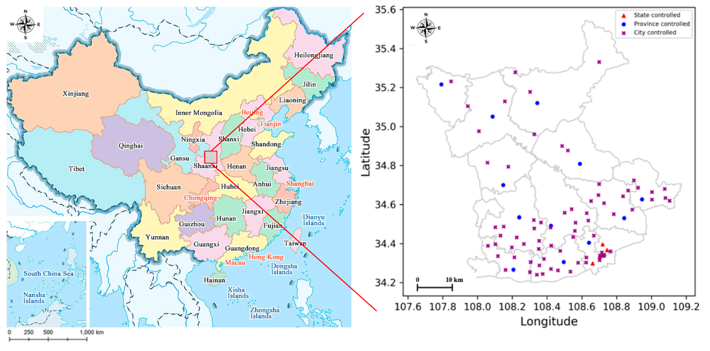
2.1. Data Collection

Data for this analysis was obtained from China National Environmental Monitoring Center (CNEMC) and Shaanxi Air Quality Real-time Publish System (SAQRPS). CNEMC has been publishing hourly monitoring data of the concentrations of six air pollutants, including PM_2.5, through an online reporting portal [24] for all the state-controlled monitoring sites in China. SAQRPS’s database [25] includes all data of province-controlled and city-controlled monitoring sites in Shaanxi Province. We collected all the monitoring sites data of Xianyang from CNEMC and SAQRPS, which includes 89 sites totally. There are d state-controlled, 12 province-controlled and 73 city-controlled monitoring sites. Monitoring data for each site was hourly time series data from 1 January 2018 to 12 February 2020. Figure 1 presents the location of Xianyang and all its monitoring sites. Xianyang locates in the Guanzhong Plain, which is the national key air pollution prevention area. Previous studies were mostly based on state-controlled monitoring sites data, but the state-controlled monitoring sites account for only 4.5% of the total sites in Xianyang. From the perspective of spatial distribution, the state-controlled monitoring sites locate in the southeast of Xianyang and concentrated on a small area, so it cannot represent the situation of the entire city. Therefore, we imposed province-controlled and city-controlled monitoring sites data into this study to make accurate spatial analysis of PM_2.5. The missing value rate for all sites was between 2% to 9%. The sample with a missing value will be removed when we calculated the distance and correlation for sites, and later we will discuss the impact of missing value.

Since we are proposed to distinguish the different air pollution areas of Xianyang, we selected the PM_2.5 time series data in heavily polluted days from 1 January 2018 to 12 February 2020 and finally got 86 days in total. Most of the time (89% of days), the air quality did not meet the heavy pollution standard, and the local government did not launch the emergency plan. Therefore, we focused on the heavily polluted days to delineate the boundaries of PM_2.5.

2.2. Data Preparation

A spatially adjacent matrix needs to be constructed before we cluster the sites. In the first step, we calculated the spatial distance for each pair of the sites and sorted the distances in ascending order, thus we got a distance vector for each site (Equation (1)). The distance between each site and itself is zero. In the second step, we constructed the spatial adjacent matrix by Equation (2) with parameter k = 10, which means we selected the k nearest neighbors of each site to construct the adjacent matrix. The reason why we did not choose a specific distance to construct the adjacent matrix is that the distribution of the sites was uneven. Some sites are much closer, and some are far away. Later in the sensitivity analysis part, we will discuss the stability of results for different parameters of k. The spatial adjacent matrix is a binary matrix with element either 1 or 0, where 1 indicates the pair of sites are adjacent and 0 indicates the pair of sites are not adjacent. This study assumed only adjacent sites can be grouped together. Finally, we got a symmetric spatial adjacent matrix with dimension 89 × 89. The calculation was performed using Python v3.7.1.

Equation (1) Distance vector for site i

$$d_i={\left(0, d_i^1,d_i^2,\dots ,d_i^n\right)}^T$$

(1)

where:

$d_i^k$ represents the k-th smallest distance;

n represents the number of sites minus one.

Equation (2) Spatial adjacent matrix

$$A_{i,j}=\{\begin{array}{cc}1& \mathrm{if} i\ne j \mathrm{and} d_{i,j}\le d_i^k\\ 0& \mathrm{others}\end{array}$$

(2)

where:

$A_{i,j}$ represents the element of spatial adjacent matrix;

$d_{i,j}$ represents the distance between site i and site j

2.3. Hierarchical Clustering

Hierarchical clustering methods have been widely adopted for analyzing air pollution [26]. These methods recursively find nested clusters either in an agglomerative or divisive manner. An agglomerative hierarchical clustering algorithm is generally implemented with four steps. First, each sample is initialized to one cluster. Second, calculate the distances between clusters. Third, merge clusters with the minimum distance into one cluster. Fourth, repeat the second and third steps until there is only a single cluster. There are five different proximity measures used for merging clusters in hierarchical algorithms, they are single-linkage, complete-linkage, average-linkage, centroid-linkage, and Ward-linkage. In this study, we assumed that only adjacent sites can be grouped together, and only hierarchical clustering methods supported to impose the adjacent matrix constraint. The clustering algorithm was performed with average linkage by using the function AgglomerativeClustering in scikit-learn v0.22.1 library.

3. Results

3.1. Selecting the Number of Clusters

Most clustering algorithms need to specify the number of clusters in advance, and it is one of the primary difficulties when applying clustering algorithms to extract meaningful information and patterns. For hierarchical clustering algorithm, several criteria can help us to choose the optimal number of clusters, in which Silhouette index and Dunn index are the most often used in practice [26]. We used Silhouette index to assist us in choosing the number of clusters. Silhouette index values range from −1 to 1, and generally the large value indicates better performance of clustering. However, when there is strong correlation between samples, the Silhouette index cannot get very close to 1. Practically, the optimal number of clusters mostly depends on the relative ranking of Silhouette index. It means choose the number of clusters that has the biggest Silhouette index. Figure 2 presents the relation between the number of clusters and Silhouette index, and two clusters were selected as the optimal number of clusters as it represented the maximal Silhouette index.

3.2. Delimit the Polluted Regions

All 89 monitoring sites were classified into two clusters (Figure 3). Cluster 1 composed of 48 sites located in the south of the city, shown in red color. Cluster 2 composed of 41 sites located in the north of the city, shown in blue color. These two clusters were separated completely because of a connection constraint imposed in the hierarchical cluster algorithm. This was very crucial in delimiting the polluted regions for the city. A Voronoi diagram was generated for each monitoring site based on its location. The Voronoi diagram is a partition for the geographic space of the city into small areas where each area contains only one site. And any point in the area has the shortest distance with the site in the same area than any other sites not in the same area. The Voronoi diagram has been widely used in many fields, such as humanities, biology, geometry, and so on. The small areas in the same cluster were merged into one single region, which was considered the polluted region for PM_2.5. Xianyang was divided into two regions from a PM_2.5 pollution perspective. The boundary generated by Voronoi diagram had many sharp corners and needs to be smooth for better cartographic presentation. We used Chaikin’s corner-cutting algorithm to smooth the boundary. In the last, we got the two polluted regions and a smoothing boundary across the city from west to east.

3.3. Correlation Analysis

The correlation coefficients for all sites were presented in groups as correlation heat maps in Figure 4. The greener the color means the more relevant between sites. It showed that sites are much more relevant within the cluster and less relevant between clusters. The more bigger correlation coefficients in the same cluster and smaller correlation coefficients between clusters means the better performance of clustering algorithm. The average correlation coefficient is 0.61 in cluster 1 and 0.62 in cluster 2, much larger than 0.31 between two clusters.

4. Discussion

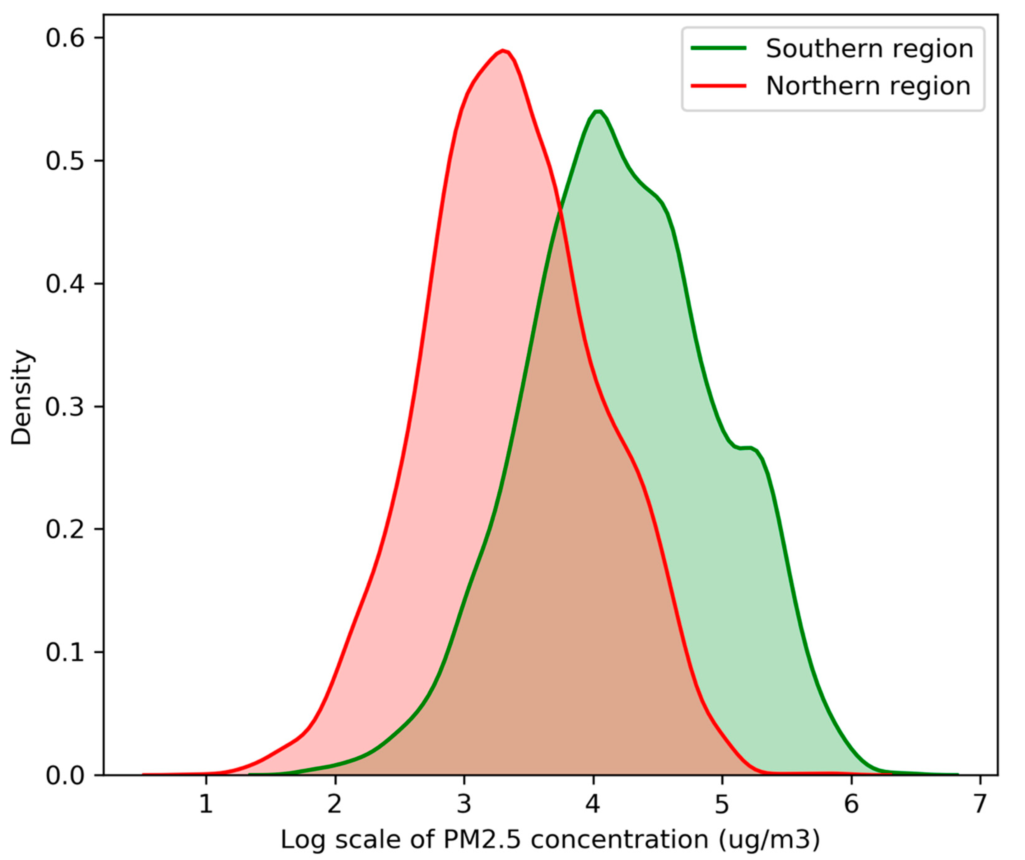
4.1. PM_2.5 Concentration in Different Region

The PM_2.5 concentration was quite different between the south and north regions. The average PM_2.5 concentration in the south was 66 μg/m³ from 1 January 2018 to 12 February 2020, while that was 49 μg/m³ in the north (Figure 5). The south was 35% higher than the north. The standard deviations were 51 μg/m³ and 49 μg/m³ respectively. The raw PM_2.5 concentration was log transformed to satisfy the normal distribution condition. The two sample T-test indicated the p-value was 4.6 × 10⁻¹³³, which means there was a significant difference between two regions and the PM_2.5 pollution in southern region was much serious. Furthermore, there were 250 polluted days (32% of all days) polluted in the southern region and 117 days more than the north according to the standards in Technical Regulation on Ambient Air Quality Index Daily Report. There were 64 days (8% of all days) of heavy and serious pollution in south and about six times more than the north. From 1 January 2020 to 12 February 2020, there were already 12 heavy and serious polluted days in the southern region and only 1 heavy polluted day in the northern region. Xianyang had started level two emergency response from 9 January 2020 to 14 January 2020. It included 10 mandatory emission reduction policies for the whole city, such as special vehicle prohibition, open-air operation prohibition, construction materials plant shutdown, no outdoor sports in school and so on. The results in this paper showed the northern region contributed very little to the PM_2.5 pollution, so there would be less economic loss if there was Air Quality Manage District policy based on the polluted regions.

4.2. Comparison to Administrative Districts

Since the southern region was the most polluted area in Xianyang and heavy PM_2.5 pollution most likely happened in this region, the Air Quality Management District policy based on the polluted region would be the key method to minimize pollution emission while reducing social and economic damage. The results showed the PM_2.5-polluted regions were distributed across the administrative districts in Xianyang. There were four administrative districts almost completely located in the southern region (

Table 1. Key social and economic indicators of administrative districts in Xianyang in 2018.

District	Area (km2)	Southern (%)	Northern (%)	Population (Thousand)	Population Density (per km2)	GDP (Billion)	Industry GDP (Billion)	Number of Primary and Junior Schools
Qindu	129	99.6%	0.4%	351	2729	38.3	24.9	58
Weicheng	17	100.0%	0.0%	213	12524	37.9	29.2	27
Sanyuan	577	55.1%	44.9%	412	714	24.0	14.3	78
Jingyang	569	72.4%	27.6%	315	554	7.5	1.3	79
Qianxian	1000	3.8%	96.2%	536	536	17.4	7.2	76
Liquan	1011	14.3%	85.7%	456	451	16.1	4.9	62
Yongshou	888	0.0%	100.0%	189	213	8.5	3.8	66
Changwu	570	0.0%	100.0%	172	302	10.0	6.3	45
Xunyi	1774	0.0%	100.0%	268	151	9.7	4.6	77
Chunhua	983	0.0%	100.0%	198	201	7.6	2.7	36
Wugong	392	95.9%	4.1%	417	1065	14.1	6.7	89
Xingping	453	99.9%	0.1%	506	1116	24.8	13.5	100
Binzhou	1181	0.0%	100.0%	333	282	21.7	15.7	146

), they were Qindu (99.6%), Weicheng (100%), Wugong (95.9%) and Xinping (99.9%). There were six administrative districts almost located in the northern region, Qianxian (96.2%), Yongshou (100%), Changwu (100%), Xunyi (100%), Chunhua (100%), and Binzhou (100%). The other three administrative districts were located both in the southern and northern region. The southern region takes only a quarter of the city area while the north region takes three quarters. The results made it very convenient for policy makers to delimit Air Quality Management District. The city could be divided into a southern and northern region. The southern region includes four administrative districts completely and three administrative districts partly, while the northern region includes six administrative districts completely and the rest of the three districts. It also suggested there should be two stages for the implementation of emergency response when heavy air pollution happened. Stage 1, the southern region might implement emergency management response first and the northern region remains the same as usual. Stage 2, when the pollution spreads across the city, the northern region should also implement the emergency response.

4.3. Social and Economic Impact Analysis

The social and economic activity would suffer a significant impact when the emergency management response was implemented. Only if we can implement air quality management by pollution region, we could minimize the damage to our society and economy. The data showed (Table 1) the southern region had about 2 million people (46%), while there were 2.3 million (54%) in the north. It means 2.3 million people and 557 primary and junior schools (59%) will not be impacted, if pollution could be controlled in stage 1. The northern region contributes 102 billion GDP (43%) and 51 billion industry GDP (38%), and its economy will also not be impacted in stage 1. Xianyang had started level two emergency response from 9 January 2020 and lasted for 6 days. However, the only day heavy pollution happened in the north was 25 January 2020. The northern region had not met the conditions of emergency response during this period. This indicates it is very necessary to implement Air Pollution Management District to make the policy more accurate and scientific.

Qindu, Weichang are core districts of Xianyang. These two core districts take less than 2% of area, 13% of population and 32% of GDP of Xianyang. In addition, the population density is 3872 per km², about nine times higher than the average level of Xianyang. Although these two districts are very important and all the state-controlled monitoring sites are located in these two districts, they still could not represent the whole city because these two districts all locate in the south of Xianyang. The southern region is mainly plain terrain with lower altitude, and the north region is mainly plateau terrain with higher altitude. The highest altitude is 1826 m in the north east and the lowest altitude is 366 m in the south. The huge terrain difference in Xianyang indicates different pollution prevention and control measures are needed in the south and north regions.

4.4. Spatiotemporal Characteristics

The pollution process (Figure 6) during level two emergency response in 2020 revealed the big difference in spatiotemporal characteristics between these two regions. PM_2.5 pollution first happened in south west of the city and then spread to the southern region. The average PM_2.5 concentration in the southern region was always greater than 150 μg/m³ during the emergency response period, and even more than 250 μg/m³ sometimes in some parts of the southern region. Although the pollution spread gradually to the north, the northern region did not suffer heavy pollution. The northern region had medium pollution on 9 January 2020 and 12 January 2020 with PM_2.5 concentration between 118 μg/m³ to 130 μg/m³, light pollution in 13 January 2020 and moderate for the remaining 3 days. From 14 January 2020, air quality was getting better from north east to south west gradually. The northern region did not meet the conditions of emergency response but still started to implement the very strict emission reduction policy. It might be more reasonable to manage the air quality by regions with different levels of prevention measures. Since heavy air pollution often occurs in the southern region, the southern region should implement more strict reduction policy, while the north should implement less strict reduction policy. In an optimistic scenario, to implement emergency response in the south is enough to mitigate the heavy PM_2.5 pollution.

5. Sensitivity Analysis

5.1. Invariance against Missing Data

During actual operation, the monitoring instruments may have problems with unknown causes, which lead to missing data for the site. We randomly dropped 10% of the whole data to simulate this situation and regrouped all the sites into two clusters. This process was repeated 100 times. The clustering results of each test were compared to the original results using Adjusted Rand Index (ARI). The mean agreement between the testing clustering results and the original was adequate with ARI 0.83. In 78% of the cases, ARI were exactly equal to 1, which means the missing value did not affect the clustering at all. This suggests that the regional boundary obtained in this study has a strong invariance property against the missing data. In this study, we just removed the samples with missing values when we calculated the correlation of monitoring sites. Since it is a big topic of how to deal with missing values in both environmental and other domains, it is very meaningful to fill or estimate the missing values in the data process in further research.

5.2. Invariance against Pollution Degree

Heavy pollution is the most important issue of our concerned, and it is the reason we selected our data to be clustered. Experiments were also conducted under severe pollution (PM_2.5 concentration greater than 250 μg/m³), medium pollution (greater than 115 μg/m³) and light pollution (greater than 75 μg/m³) conditions in this study to test the invariance property against pollution degree. The ARI result of heavy pollution between severe pollution was 1.0, 0.91 between medium pollution, and 0.71 between light pollution. This suggests that the clustering result is robust again the different pollution degrees, which is very important for the air pollution region recognition.

5.3. Invariance against k Parameter and Linakge Function

Parameter k was used when constructing the spatial adjacent matrix. If the distance between sites was less than the k-nearest distance, then the sites were adjacent or neighbors and only adjacent sites could be grouped into the same cluster. We imposed the constraint to get a continuous region. Parameter k was selected from 5 to 20 and cluster process was recalculated. ARI were calculated for the combinations of k. We found that ARI were very stable for k from 7 to 13, the average ARI was 0.9. However, when k was smaller than 7 and bigger than 13, ARI dropped to 0.4 rapidly. We chose k equals 10 for stable cluster results. Another consideration is how linkage function affects the cluster results. We chose single-linkage, complete-linkage and Ward-linkage respectively to compare with the results of average-linkage we used in this study. The results showed the ARI of single-linkage and complete-linkage was 0.83 and 0.84, respectively, and Ward-linkage was 0.61. The results of single-linkage, complete-linkage and average-linkage were based on the distances of each observation, and Ward-linkage aimed to minimize the variance of the clusters that merged.

6. Conclusions

All the monitoring sites of Xianyang were grouped into two clusters by using hierarchical clustering algorithm under the connection constraint. The two polluted regions were delimited by Voronoi diagram and Chaikin’s corner-cutting algorithm for the city, the southern and northern region. The southern region consisted of four administrative districts completely and three partly; it took about one quarter of the area of Xianyang. The northern region consisted of the other six administrative districts completely and three partly. The southern region was polluted for 32% of the time since 1 January 2018 while only 14% in the northern region. The days of heavy polluted or more serious were six times more in southern region than that in the northern region. It could greatly reduce the damage to society and economy if there is Air Quality Management District policy based on the polluted region delimited in the study. Seventy-five percent of the city area, 2.3 million people, 59% of schools, and 43% of GDP would not be impacted by the emergency plan because the northern region contributed very little to the pollution.

References

1. Chen, Z.; Cai, J.; Gao, B.; Xu, B.; Dai, S.; He, B.; Xie, X. Detecting the causality influence of individual meteorological factors on local PM2.5 concentration in the Jing-Jin-Ji region. Sci. Rep. 2017, 7, 40735. [Google Scholar] [CrossRef] [Green Version]
2. Deng, Q.; Yang, K.; Yi Luo, Y. Spatiotemporal Patterns of PM2.5 in the Beijing–Tianjin–Hebei Region during 2013–2016. Geol. Ecol. Landsc. 2017, 1, 95–103. [Google Scholar] [CrossRef]
3. Di, Q.; Kloog, I.; Koutrakis, P.; Lyapustin, A.; Wang, Y.; Schwartz, J. Assessing PM2.5 Exposures with High Spatiotemporal Resolution across the Continental United States. Environ. Sci. Technol. 2016, 50, 4712–4721. [Google Scholar] [CrossRef] [PubMed] [Green Version]
4. Govender, P.; Sivakumar, V. Application of k-means and hierarchical clustering techniques for analysis of air pollution: A review (1980–2019). Atmos. Pollut. Res. 2020, 11, 40–56. [Google Scholar] [CrossRef]
5. Hill, L.; Edwards, R.; Turner, J.R.; Argo, Y.D.; Olkhanud, P.B.; Odsuren, M.; Guttikunda, S.; Ochir, C.; Smith, K.R. Health assessment of future PM2.5 exposures from indoor, outdoor, and secondhand tobacco smoke concentrations under alternative policy pathways in Ulaanbaatar, Mongolia. PLoS ONE 2017, 12, e0186834. [Google Scholar] [CrossRef] [PubMed]
6. Huang, H.; Fu, D.; Qi, W. Effect of driving restrictions on air quality in Lanzhou, China: Analysis integrated with internet data source. J. Clean. Prod. 2017, 142, 1013–1020. [Google Scholar] [CrossRef]
7. Li, L.; Wu, A.H.; Cheng, I.; Chen, J.-C.; Wu, J. Spatiotemporal estimation of historical PM 2.5 concentrations using PM 10, meteorological variables, and spatial effect. Atmos. Environ. 2017, 166, 182–191. [Google Scholar] [CrossRef]
8. Li, L.; Zhang, J.; Meng, X.; Fang, Y.; Ge, Y.; Wang, J.; Wang, C.; Wu, J.; Kan, H. Estimation of PM2.5 concentrations at a high spatiotemporal resolution using constrained mixed-effect bagging models with MAIAC aerosol optical depth. Remote Sens. Environ. 2018, 217, 573–586. [Google Scholar] [CrossRef]
9. Liu, J.; Li, W.; Wu, J. A framework for delineating the regional boundaries of PM2.5 pollution: A case study of China. Environ. Pollut. 2018, 235, 642–651. [Google Scholar] [CrossRef]
10. Liu, X.; Chen, Q.; Che, H.; Zhang, R.; Gui, K.; Zhang, H.; Zhao, T. Spatial distribution and temporal variation of aerosol optical depth in the Sichuan basin, China, the recent ten years. Atmos. Environ. 2016, 147, 434–445. [Google Scholar] [CrossRef]
11. Samet, J.M.; Dominici, F.; Curriero, F.C.; Coursac, I.; Zeger, S.L. Fine Particulate Air Pollution and Mortality in 20 US Cities, 1987–1994. N. Engl. J. Med. 2000, 343, 1742–1749. [Google Scholar] [CrossRef]
12. Shen, Y.; Zhang, L.; Fang, X.; Ji, H.; Li, X.; Zhao, Z. Spatiotemporal patterns of recent PM2.5 concentrations over typical urban agglomerations in China. Sci. Total Environ. 2019, 655, 13–26. [Google Scholar] [CrossRef]
13. Song, C.; He, J.; Wu, L.; Jin, T.; Chen, X.; Li, R.; Ren, P.; Zhang, L.; Mao, H. Health burden attributable to ambient PM2.5 in China. Environ. Pollut. 2017, 223, 575–586. [Google Scholar] [CrossRef]
14. Viard, V.B.; Fu, S. The effect of Beijing’s driving restrictions on pollution and economic activity. J. Public Econ. 2015, 125, 98–115. [Google Scholar] [CrossRef] [Green Version]
15. Wang, B.; Liu, S.; Du, Q.; Yan, Y. Long Term Causality Analyses of Industrial Pollutants and Meteorological Factors on PM2.5 Concentrations in Zhejiang Province. In Proceedings of the 2018 5th International Conference on Information Science and Control Engineering (ICISCE), Zhengzhou, China, 20–22 July 2018; Institute of Electrical and Electronics Engineers (IEEE): Piscataway, NJ, USA, 2018; pp. 301–305. [Google Scholar]
16. Wang, L.; Zhang, F.; Pilot, E.; Yu, J.; Nie, C.; Holdaway, J.; Yang, L.-S.; Li, Y.; Wang, W.; Vardoulakis, S.; et al. Taking Action on Air Pollution Control in the Beijing-Tianjin-Hebei (BTH) Region: Progress, Challenges and Opportunities. Int. J. Environ. Res. Public Health 2018, 15, 306. [Google Scholar] [CrossRef] [Green Version]
17. Xu, H.; Ho, S.S.H.; Gao, M.; Cao, J.; Guinot, B.; Ho, K.F.; Long, X.; Wang, J.; Shen, Z.; Liu, S.; et al. Microscale spatial distribution and health assessment of PM2.5-bound polycyclic aromatic hydrocarbons (PAHs) at nine communities in Xi’an, China. Environ. Pollut. 2016, 218, 1065–1073. [Google Scholar] [CrossRef]
18. Xu, Y.; Ying, Q.; Hu, J.; Gao, Y.; Yang, Y.; Wang, D.; Zhang, H. Spatial and temporal variations in criteria air pollutants in three typical terrain regions in Shaanxi, China, during 2015. Air Qual. Atmos. Health 2017, 11, 95–109. [Google Scholar] [CrossRef]
19. Yan, D.; Lei, Y.; Shi, Y.; Zhu, Q.; Li, L.; Zhang, Z. Evolution of the spatiotemporal pattern of PM2.5 concentrations in China–A case study from the Beijing-Tianjin-Hebei region. Atmos. Environ. 2018, 183, 225–233. [Google Scholar] [CrossRef] [Green Version]
20. Yuan, Y.; Liu, S.; Castro, R.; Pan, X. PM2.5 Monitoring and Mitigation in the Cities of China. Environ. Sci. Technol. 2012, 46, 3627–3628. [Google Scholar] [CrossRef]
21. Zhan, Y.; Luo, Y.; Deng, X.; Chen, H.; Grieneisen, M.L.; Shen, X.; Zhu, L.; Zhang, M. Spatiotemporal prediction of continuous daily PM2.5 concentrations across China using a spatially explicit machine learning algorithm. Atmos. Environ. 2017, 155, 129–139. [Google Scholar] [CrossRef]
22. Zhang, D.; Zhang, M.; Zhang, B. Study on the Response of PM2.5 Pollution to Different Geographical Factors. In Proceedings of the 2018 26th International Conference on Geoinformatics, Kunming, China, 28–30 June 2018; Institute of Electrical and Electronics Engineers (IEEE): Piscataway, NJ, USA, 2018; pp. 1–5. [Google Scholar]
23. Zhao, S.; Yu, Y.; Yin, D.; Qin, D.; He, J.; Dong, L. Spatial patterns and temporal variations of six criteria air pollutants during 2015 to 2017 in the city clusters of Sichuan Basin, China. Sci. Total Environ. 2018, 624, 540–557. [Google Scholar] [CrossRef] [PubMed]
24. National Air Quality Data Release System. Available online: http://106.37.208.233:20035/ (accessed on 10 August 2020).
25. Shaanxi Air Quality Real-time Publish System. Available online: http://113.140.66.226:8024/sxAQIWeb/PageCity.aspx?cityCode=NjEwNDAw (accessed on 10 August 2020).
26. Zhuang, Y.; Chen, D.; Li, R.; Chen, Z.; Cai, J.; He, B.; Gao, B.; Cheng, N.; Huang, Y. Understanding the Influence of Crop Residue Burning on PM2.5 and PM10 Concentrations in China from 2013 to 2017 Using MODIS Data. Int. J. Environ. Res. Public Health 2018, 15, 1504. [Google Scholar] [CrossRef] [PubMed] [Green Version]
Figure 1. Geographical location of Xianyang and monitoring sites.
Atmosphere 11 00972 g001
Figure 2. Choice of the optimal number of clusters.
Atmosphere 11 00972 g002
Figure 3. Smoothing boundary between these two clusters. The light red region is generated by the sites in cluster 1, and the light blue region is generated by the sites in cluster 2. The black smoothing curve was generated by Chaikin’s corner-cutting algorithm.
Atmosphere 11 00972 g003
Figure 4. Correlation heat map of all the sites in groups. The sites were numbered from 0 to 88. Cluster 1 includes number 0 to number 47, while cluster 2 includes number 48 to number 88.
Atmosphere 11 00972 g004
Figure 5. Density of PM2.5 concentration in southern and northern region.
Atmosphere 11 00972 g005
Figure 6. Heavy pollution process during level two emergency response days in 2020. 9 January 2020 (a), 10 January 2020 (b), 11 January 2020 (c), 12 January 2020 (d), 13 January 2020 (e) and 14 January 2020 (f).
Atmosphere 11 00972 g006