1. Introduction
A problem of a wave mode identification has interdisciplinary character, it is important, for example in physics of atmosphere, where superposition of acoustical, gravity and planetary waves occur [
1]. In planetary range the periods of Rossby and Poincare waves are of the same scale, hence their separation and estimation of contributions is complicated [
1]. Similar problem relates to the distinction between acoustic and internal gravity waves [
2]. The situation is even more complicated in plasma physics for additional specific branches of waves coexist with ones for neutral gas. An important problem of a specific mode source localization is also typical inverse problem that is generally ill-posed [
3].
In geophysics the wave field diagnostics, based on dispersion relations, conventionally needs many observations that cover a space enough for wave length estimation. It is rather expensive and not very feasible.
The alternative wave or non-wave (zero frequency) modes identification is based on the relation between the state vector components. mathematically it is determined via eigenvalue problem for evolution operator. The frequency then play the role of a corresponding eigenvalue. It is convenient to use for each such eigenvector space a projecting operator, that is uniquely defined, and split the evolution problem, simplifying it. Such a technique is properly described for initial problems [
4]. The next alternative, with similar properties, but more convenient for direct observations is based on eigenvectors of a coordinate evolution operator. Such vectors are fixed by relation between components as well, but at a boundary. The corresponding eigenvalues now serve as the wavenumbers. Thinking about this novel alternative approach [
5] we suggest using measurements in a vicinity of a point but many-components observations with aid of the projecting operators, corresponding to the mentioned boundary problem. So, the technique built in this article, fit subspaces of specific wave and non-wave modes.
To speak about an instructive example of 1D wave (string) equation and corresponding Cauchy problem we can address, see for example [
6,
7]. Naturally a dispersion or dissipation complicates the situation but may be overcome [
4,
8]. Weak inhomogeneities of propagation media may be also effectively included in similar manner [
9].
There are lot of important problems in theoretic physics of the same level of description: for electrodynamics see [
10,
11] for acoustic [
12,
13], and Tollmienn–Schlichting waves [
14], that may be directly formulated as the system of equations so the vector description (in electrodynamics those are six field components) have direct physical sense. We must mention however that the directed waves correspond to a combination of electric and magnetic field, so-called hybrid variables with appropriate initial or boundary conditions [
10].
More complicated 3D problems need more advanced constructions and geometry (ring or sphere in geophysics [
5]), its impact may lead to very nontrivial generalization of the technique and algorithm as well as norm of the appropriate spaces construction. Our present study is focused on the simplest 1+1 case, that includes one space and one time coordinate restricting ourselves by exponential atmosphere model.
The technique of projecting operator apart from formal division of solutions space to mode subspaces should be supplied with a tool for estimation of errors, implemented by physical errors of measurements and an estimation of diagnostics quality in a finite number of available measurements realization. In our case these are perturbations of the temperature and density of the atmosphere gas. Each sequence of the measurements results may be considered as a finite-dimensional vector, that approximate a solution, that, naturally is given by functions, which, naturally, are elements of an infinite-dimensional space. In both spaces we use a scalar product and norm that are of similar origin, used in so-called unitary spaces. Its norm used for an error estimation looks as mean squared deviation. The explicit expression for such a norm in this space is determined via expression for energy, that have quadratic form in terms of wave variables and conserves. Hence we could estimate the diagnostics errors, to be used in energy balance study, and, next, it gives a quality of a wave source position determination.
We fix our attention on the minimal version of the one-dimensional acoustic wave theory to show the main idea of a wave diagnostics, may be most characteristic for the opposite propagating waves.
In this 1+1 case the wave type (defined as relation between temperature and density perturbations, named as “polarization” in an analogy with the known property of light) is linked to direction of propagation, marked by the wavenumber.
The projecting operator technique is used to split the solution space and analyze input of a wave monitoring in a vicinity of an observation point. The solution space is supplied by a norm with properties of one for unitary space, more particular-the energy one, supported by the conservation law; its finite-dimensional analog, obtained by discretization, is used as a measure of a given mode presence. For the projecting operators construction we use 1D problem of the acoustic wave initiation by a boundary condition. The operators are applied to the results of measurements of the temperature and density of the neutral atmosphere in the range height 90–120 km by API (method of resonant scattering of radio waves by artificial periodic irregularities of the ionospheric plasma) technique. The entropy or zero frequency mode account in the problem of acoustic waves extraction is also discussed in terms of corresponding projecting technique. The reformulation of a problem that fix eigen subspaces of evolution operator is shown. Projecting to subspaces and their weights evaluation in an appropriate physical norm for the functional and finite-dimensional spaces is realised. It allows us to formulate mathematically the whole algorithm of wave diagnosis, we sketch below for readers convenience.
The z-evolution equation of a two-component vector state
is
namely such a form that is derived in
Section 2 defines the evolution operator
L. The notations differ because the dimensionless coordinates and entropy (instead of temperature) are introduced for compactness.
The eigenvalue problem for the evolution operator
L after Fourier transformation in
t takes the matrix form
For each eigenspace
it is convenient to introduce the projecting operators by means of the 2 × 2 matrix
,
so that [
4]
that is the functions of the frequency
.
To apply the projecting technique to the observation data, we transform the data by discrete Fourier transformation and, next use the corresponding discretized projecting matrices to extract the data for two modes (directed waves)
The energy of the directed waves are estimated by discretized form of the general expression for acoustic waves energy, known as a direct corollary of the basic evolution system.
In experiments carried out based on the SURA mid-latitude heating facility for API creation, many parameters of the neutral and ionized components of the ionosphere at altitudes of 60–120 km were determined. For more than 35 years of the regular research by API technique, the physical processes of the API formation under the action of a powerful standing wave have been studied. We use resonant scattering of radio waves by artificial periodic irregularities of the ionospheric plasma as a method for determining many parameters of the lower ionosphere. The most important of them are atmospheric temperature and density at height in the range 85–120 km, vertical motion velocity, the intensity of the turbulence and velocity of the turbulent motion at height 60–120 km, the height profile of the electron density, sporadic-E layer parameters and others. Methods for determining these parameters are presented in sufficient detail in the monograph [
15]. They are based on measuring of the amplitude and phase of the API signals scattered at the stage of their disappearance (relaxation) after the end of the impact on the ionosphere by the powerful radio emission from the SURA facility. At the relaxation stage, the amplitude of the API scattered signal at the height range of 90–120 km decreases in the process of ambipolar diffusion [
16]. The atmospheric temperature and density are determined from the API relaxation time, which is inversely proportional to the ambipolar diffusion coefficient. Many results of studying the altitude–temporal variations of temperature and density in different geo- and helio-physical conditions are presented in [
17,
18,
19,
20,
21,
22,
23,
24].
The algorithm presented in 1–3 positions is realized in the
Section 2 for the boundary problem for the conventional exponential atmosphere system example. The data for such problem formulation are taken from SURA experiment [
17,
18],
Section 3 and the step 4 is done in the
Section 4. The energy estimation as the last step of the algorithm is performed in the
Section 5. A development of the theory with entropy mode account is presented in
Section 6.
The algorithm presented in this paper is derived using model for non-dissipative exponentially stratified atmosphere with low ionization. As mentioned above, we are solving problem of diagnostics, therefore this limitations need to be applied only locally. Atmosphere can be described as locally exponential nearly anywhere. At altitudes of about 100 km, where we get atmospheric data by the API technique, the not dissipative and low ionization approximation should work reasonably well. For heights where this approximation fails, the algorithm presented in the article cannot be applied as is, but it can be reformulated by obtaining a different set of projection operators using a more accurate and therefore more complex model.
Finally, we outline the text as follows:
In the
Section 2 we reformulate basic time-evolution hydro-thermodynamic system into the reduced coordinate-evolution system, that exclude entropy mode from consideration. The projecting operators that fix directed waves hybrid variables are built.
In the
Section 3 we present the results of density and temperature perturbations measurements in the active artificial periodic irregularities technique experiment.
The
Section 4 demonstrates how applications of the projecting operators splits the space of acoustic waves superposition to the directed ones.
The
Section 5 is devoted to derivation of expression for mode energy and its calculations.
In the
Section 6 we return to the full hydrothermodynamic system to include the entropy mode and derive three projecting operators for the directed acoustic waves and entropy modes.
Final
Section 7 contains the general expression for energy and its division to the three modes contributions.
The conclusion
Section 8 summarizes the work and outline the perspective of its development, including more detailed description of the modes profiles.
2. Two-Mode Problem
Following [
15] we start with standard hydrothermodynamic system describing deviation of pressure
, density
and velocity
U from equilibrium values
where
and
are the air density and pressure at the zero height and
is the adiabatic constant,
z is a height and
H is the height of uniform atmosphere,
- mean velocity.
The linearized 1D equations for perturbations of pressure
, density
and gas velocity
there are rewritten using variable
and then we can switch to the variables, conventionally used for the exponentially stratified atmosphere model:
then the system takes the form
Systems (
2)–(
4) describe a three-mode problem with two wave modes and one stationary entropy mode. Let us first simplify it by getting rid of entropy mode. To do it we can take
U from the third equation in the form
and plug it into the Systems (
2)–(
4)
giving us the system describing two oppositely directed wave-modes
Then
z-evolution operator takes the form
Let us rewrite it in the terms of dimensionless functions and variables and also go from Cauchy problem to boundary mode propagation problem. For this we will use the uniform atmosphere height
H and the speed of sound
as dimension parameters which gives us time scale
so that the new dimensionless variables are
,
. Functions are redefined as
,
and, since the
too has the pressure as a dimension (because
and
) and
giving us system
To simplify the result we can choose
where
is an arbitrary parameter and then find value of
which ensures that coefficient before the term
is always zero. It happens when
Both solutions would work, but
is simpler. In this case the systems (
11) and (
12) takes form
and
Accidentally it means that we had returned to the density in our variables since .
It is now possible to extract an evolution operator in
domain for the boundary mode propagation problem (
14) and (
15). It is expressed as the matrix
Now it is possible by following standard procedure [
4] (introduced for acoustic waves in [
2]) to obtain an projection operators:
where
,
.
So, we have projection operators. However, they are calculated in the -space, while boundary conditions are usually known in -space (at ). We need either transform projection operators back into -space or transform boundary conditions into -space. The last option looks a lot easier than former.
3. Atmospheric Data for Analysis from SURA Observations
The wave diagnostics algorithm (see introduction 1–5,) considered in
Section 2 is applied to the analysis of real measurements of the temperature and density of the neutral component, made by the method of resonant scattering of radio waves by artificial periodic irregularities of the ionospheric plasma (APIs). The experiments were carried out at the SURA heating facility (56.11° N; 46.1° E) which is situated near Nizhny Novgorod, Russian Federation. It is used to affect the ionosphere by high-frequency radio waves with a rated effective power of up to 350 MW and create artificial disturbances in the ionosphere influenced on a radio wave propagation. Powerful radio waves radiated into the ionosphere disturb the temperature and concentration of electrons. This causes many different “heating” effects in the ionospheric plasma, which are described in detail in reviews [
16,
20]. The creation of artificial periodic irregularities in the field of a powerful standing radio wave is among them. The API technique is described in detail in [
21]. Here we briefly outline the main features of this method.
To learn more about the API technique and in detail the methodology for determining the atmospheric temperature and density, we recommend reading [
18,
21]. Estimates show the relative perturbation of the electron density in irregularities can reach
in the E-layer and
in the D-layer for the heating frequencies 4-6 MHz and for the effective radiation power of the heating facility 80–120 MW. A large level of the scattered signal with a signal-to-noise ratio of the order of 10–100 is ensured by the resonant nature of the scattering of radio waves by the APIs. The method for determining the temperature and density of the neutral atmosphere based on the analysis of the height dependence of the relaxation time of the API scattered signal is described in detail in [
21]. At altitudes of 90–120 km, the API relaxation occurs under the influence of the ambipolar diffusion. The relaxation time is determined by the expression
where
is the Boltzmann constant, K =
is the wavenumber of the standing wave,
is the wavelength in the propagation medium, n is the refractive index,
D is the ambipolar diffusion coefficient,
is the molecular mass of the ion,
and
are the unperturbed electron and ion temperatures, and
is the frequency of collisions between ions and neutral molecules. It is considered that in the mid-latitude at mesosphere and the lower thermosphere heights
up to the height 120–130 km, where T is the temperature of the neutral component. The above expression for
underlies the determination of many parameters of the lower ionosphere [
21]. As mentioned above, the API relaxation E-region heights (90–120 km) of the ionosphere is going on by the process of the ambipolar diffusion. According to Formula (
19), the ambipolar diffusion coefficient D and the special scale of the irregularities determine the relaxation time. D itself depends on the atmospheric temperature T and the collision frequency
of the ions with neutrals. The latter is proportional to the atmospheric density
, where the numeric coefficient
cm
s
[
21]. This sequences of argumentation shows the API relaxation time depends on. In each measurement session, the relaxation time
was determined from a decrease in the amplitude of the scattered signal by a factor of e at the height from 60 to 120 with a step of 0.7 or 1.4 km. Further, using Formula (
19), taking into account the dependence of the collision frequency
on the atmospheric density
, we have defined atmospheric temperature and density the atmospheric temperature and density. It allows us to determine these parameters. To learn more about the API technique and in detail the methodology for determining the atmospheric temperature and density, we recommend reading [
21,
22]. A large amount of data on the altitude–time variations in the temperature and density of the neutral component at altitudes of 90–120 km is given in [
17,
18,
21,
22,
23,
24]. In this work, we used the results of determining atmospheric parameters on 26 September 2017 from 12:00 to 16:20 local time (Moscow time).
Figure 1 and
Figure 2 shows the dependencies of the temperature and the density on dimensionless time at an altitude of 100 km. Each point on the graphs corresponds to averaging data over 5 min. The error in determining the temperature is not more than
and density error is not more than
. It can be seen in
Figure 1 and
Figure 2 that the dependencies of temperature and density on dimensionless time have a wave like character with periods from 15 min to 45–50 min. The error in determining of the temperature is not more than 10% and density error is not more than 15%. Errors are shown in figures as vertical bars.
4. Projection Operators Application
Now we have projection operators, application of them to the measurements data allows us to split a wave superposition into two separate projection, one of them to be upward-directed waves and another one for downward-directed or, in other words, to separate wave into up- and down-directed components, that is not visible in direct observations, see
Figure 1 and
Figure 2.
To apply projection operators we need to transform these data into variables of our system, scale them into dimensionless units, make discrete Fourier transformation to switch into -space.
Then we can use projecting operators
(
17) and (
18) to split the data into two modes. Some of the results of this procedure can bee seen at the
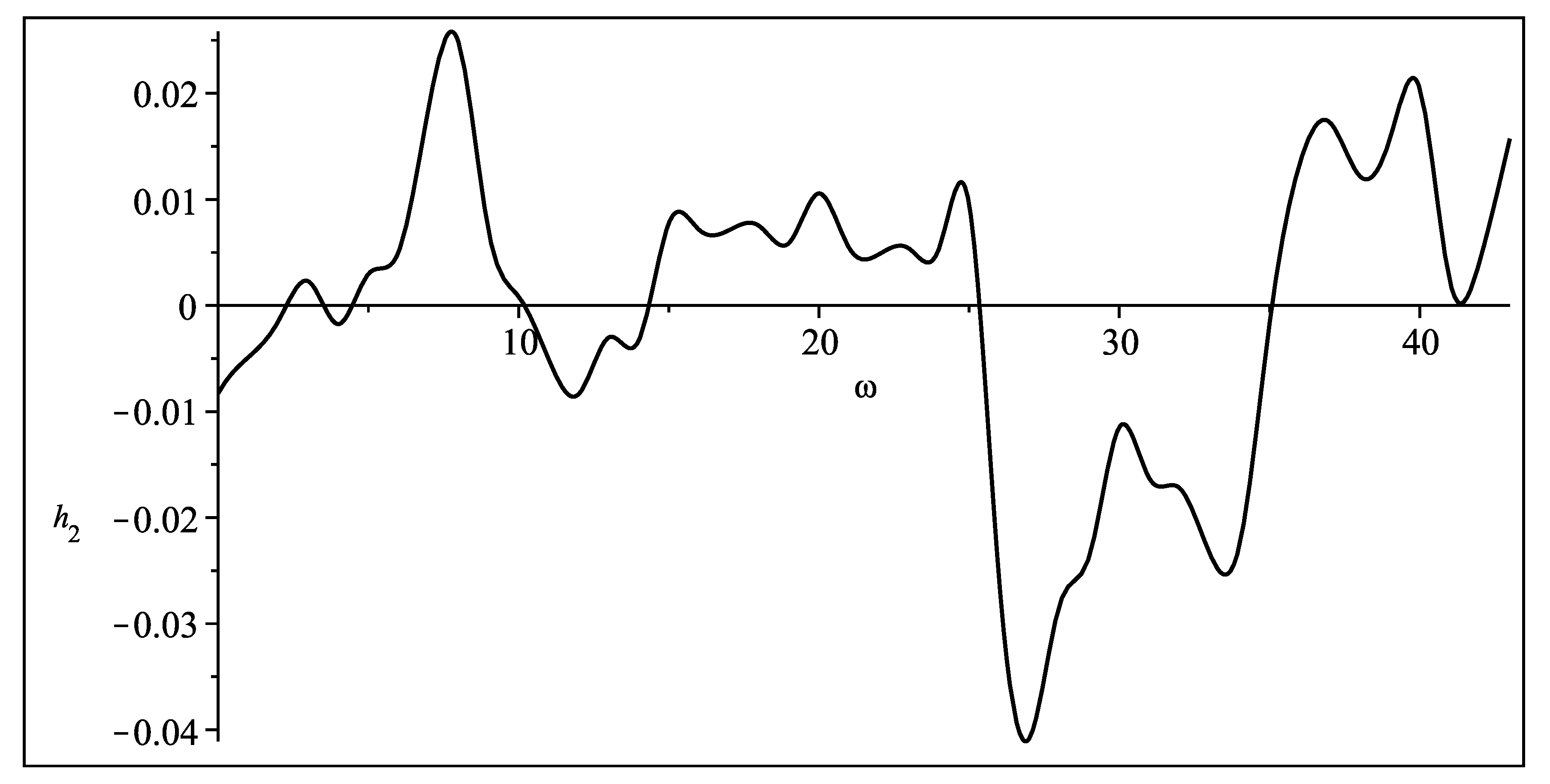
Figure 3 and
Figure 4:
We have only put graphs for the one component of each mode there since our main goal is mode energy comparison, but both real and imaginary part of both components for up- and down-ward modes were calculated.
As it can be seen, the acoustic wave frequencies are inverted for the up- and down-directed waves (as it should be in the 2-mode model), have two peaks: one localised near 7 and double peak situated around 30. In this work we do not try to investigate amplitude-frequency dependency of acoustic waves limiting ourselves to the question of energy distribution, but as
Figure 3 and
Figure 4 demonstrate, such an investigation is possible using this method. Of course, for more stringent results about this, gravity wave should be taken into account too. For now it is just result of single observation. Further work is needed to check if this results will also appear at the other observation series.
8. Conclusions
The theoretical principles for the diagnosis of atmospheric wave disturbances are described. A mathematical apparatus bases on the concept of dynamical projecting operators, that split the space of solution onto eigen subspaces of
z-evolution operator. The procedure itself consists of the projecting operators construction by means of Fourier transformation applied to the
z-evolution operator. The transform is the projecting matrix, which eigenspaces vectors form the basis for the matrix projectors conventional construction. The procedure of projection is provided by application of the discretized operator to the vector obtained by discrete Fourier transform (DFT) of the measurements data. Such a procedure allows us to diagnose disturbances that are formed by upward and downward propagating waves superposition. The measurements of the temperature and density disturbances are provided in the vicinity of observation point. The procedure is presented at the diagram below:
The paper contains three main results.
The first is the mathematical preparation of the projecting tools for the pure wave disturbances analysis. These projecting operators extract from the given data time sequence of the information about waves propagating up and down. Such a procedure implies the simultaneous measurement of two independent gas variables, in our case those are the density and temperature deviations from the equilibrium (mean value). Their measurements are performed by means of the special active experiment included the creating artificial periodic irregularities by a powerful high-frequency radio emission and the sounding them with probe radio waves, the extracting of the the necessary information about the mentioned gas parameters from time sequences of the parameters of signals scattered from the induced irregularities.
The second result allows estimating weights of such directed waves by means of calculation of the wave energies of both contributions. The division of the contribution is also extracted from the time series data by means of the projecting operators application. The result points that the contributions in the up/down directed wave energies is almost equal. This, perhaps may be explained by symmetry of reflections from the Earth surface and from "upper border" within this relatively short infra-sound from atmospheric sources.
The third result is now purely mathematical. The general one-dimensional data sequence would contain information about so-called entropy mode that shows the zero-frequency contribution in the perturbation. Such a mode may be presented due to initial/boundary condition of the overall perturbation evolution problem as well result of wave energy dissipation that in lab acoustics obtained a name of the "heating". Such data extraction implies the measurements of three dynamical variables of the atmosphere gas perturbation as the temperature, density and the vertical velocity. It is our plan for the nearest future. The entropy mode account is considered also in [
25].
There are many possible applications of the elaborated method and particular results. One of them attract serious attention in last decades under the name “warming” [
26]. The term “warming” needs a proper examination because its origin in natural observations [
27] and numerical simulations [
28] should be analyzed within the terms of entropy and other zero frequency modes. The entropy mode account is considered also in [
25]. It is known, that the contribution to momentum balance affected by waves also play a significant role in modeling and monitoring such troposphere events as cyclones. Estimation of different wave modes impact promise to be important information.
As a main perspective we plan to perform to study SURA three variables (temperature, density and velocity perturbations) measurements to investigate a contribution of the entropy mode at a superposition with upward and downward acoustics. We would mention also to study the problems of
- (a)
Wave form reconstruction for a given number of measurements and spline order choice.
- (b)
Investigation of stability in terms of explicit solution form, reconstructed by the finite points number data.
Note, the three-variables data already exists that will allow us to perform all necessary calculations in nearest future.


