Article

Generalized Description of Intermittency in Turbulence via Stochastic Methods

1
ENS de Lyon, CNRS, Laboratoire de Physique, University Claude Bernard, F-69342 Lyon, France
2
Institute for Theoretical Physics I, Ruhr-University Bochum, Universitätsstr. 150, D-44780 Bochum, Germany
*
Author to whom correspondence should be addressed.
Atmosphere 2020, 11(9), 1003; https://doi.org/10.3390/atmos11091003
Submission received: 15 August 2020 / Revised: 15 September 2020 / Accepted: 15 September 2020 / Published: 19 September 2020

Abstract

:
We present a generalized picture of intermittency in turbulence that is based on the theory of stochastic processes. To this end, we rely on the experimentally and numerically verified finding by R. Friedrich and J. Peinke [Phys. Rev. Lett. 78, 863 (1997)] that allows for an interpretation of the turbulent energy cascade as a Markov process of velocity increments in scale. It is explicitly shown that phenomenological models of turbulence, which are characterized by scaling exponents ζ n of velocity increment structure functions, can be reproduced by the Kramers–Moyal expansion of the velocity increment probability density function that is associated with a Markov process. We compare the different sets of Kramers–Moyal coefficients of each phenomenology and deduce that an accurate description of intermittency should take into account an infinite number of coefficients. This is demonstrated in more detail for the case of Burgers turbulence that exhibits pronounced intermittency effects. Moreover, the influence of nonlocality on Kramers–Moyal coefficients is investigated by direct numerical simulations of a generalized Burgers equation. Depending on the balance between nonlinearity and nonlocality, we encounter different intermittency behavior that ranges from self-similarity (purely nonlocal case) to intermittent behavior (intermediate case that agrees with Yakhot’s mean field theory [Phys. Rev. E 63 026307 (2001)]) to shock-like behavior (purely nonlinear Burgers case).

1. Introduction

The phenomenon of homogeneous and isotropic turbulence can still be considered as one of the main unsolved problems in classical physics [1,2]. An adequate treatment of the underlying Navier–Stokes equation should make an assertion about the small-scale fluctuations of the longitudinal velocity increments
δ r v ( x , t ) = u ( x + r , t ) u ( x , t ) · r r ,
in a statistical sense. Here, deviations from Kolmogorov’s mean field theory [3] that predicts ( δ r v ) n ε n / 3 | r | n / 3 are commonly attributed to the intermittent fluctuations of the local energy dissipation rate ε and manifest themselves by a non-self-similar probability density function (PDF) of the velocity increments. In turn, this implies a nonlinear order dependence for the scaling exponents ζ n of the moments ( δ r v ) n | r | ζ n . In this context, considerable efforts have been devoted to the development of phenomenological models of turbulence that all try to account for the intermittent character of the local energy dissipation rate such as the log-normal model [4,5] or the popular model by She and Leveque [6] (we also refer the reader to the monograph by Frisch [7] for further discussion).
In this paper, we follow a different phenomenological approach [8] that interprets the concept of the turbulent energy cascade, i.e., the transport of energy from large to small scales, as a Markov process of velocity increments in scale. The vigor of this phenomenology is its capability to reproduce the entire multi-scale velocity increment statistics from the integral length scale down to a scale where the Markov property is violated [9]. The experimentally and numerically verified Markov property of the velocity increments in the inertial range of scales, however, implies that the increment PDF as well as the transition PDF are governed by the same partial differential equation in scale, the so-called Kramers–Moyal expansion. As it is discussed in Section 2 of the present paper, the Kramers–Moyal approach allows for a general description of anomalous scaling. Consequently, it is able to reproduce all known phenomenological models of turbulence by the proper choice of the Kramers–Moyal coefficients that enter the Kramers–Moyal expansion.
The result of this paper is that, in order to obtain an accurate description of intermittency effects, higher order Kramers–Moyal coefficients have to be small but non-vanishing. Therefore, the truncation of the Kramers–Moyal expansion as it is done in the usual Fokker–Planck approach [8,10,11] might result in an inaccurate description of the tails of the PDFs. To this end, we investigate the asymptotics of higher-order Kramers–Moyal coefficients of the corresponding phenomenologies in Section 2.
Section 3 substantiates the existence of higher order coefficients by direct numerical simulations of the Burgers equation. Due to its advantageous properties in comparison to the Navier–Stokes equation (no nonlocal pressure contributions, integrability via the Hopf–Cole transformation [12,13]), the Burgers equation has been widely used as a model system for turbulence [14,15,16,17,18] and exhibits pronounced intermittency effects due to strong negative velocity gradients occurring in shocks (we also refer the reader to [19] for further references). Further applications of Burgers equation range from astrophysical problems [20,21,22] to solid surface growth by vapor deposition via the equivalent Kardar–Parisi–Zhang equation [23]. Moreover, the inclusion of an additional nonlocal term allows for the incorporation of intermittency effects similar to the ones that are encountered in Navier–Stokes turbulence [24]. Therefore, we will explicitly investigate the influence of the balance between nonlinearity and nonlocality and its consequences for the Kramers–Moyal coefficients. Furthermore, we will give an outlook on the extension of this analysis to ordinary Navier–Stokes turbulence.

2. Interpretation of the Turbulent Energy Cascade as a Markov Process of Velocity Increments in Scale

A key quantity in the statistical description of turbulence [2] is the n-increment PDF of longitudinal velocity increments (1) defined according to
f n ( v n , r n ; ; v 1 , r 1 ; x , t ) = i = 1 n δ ( v i δ r i v ( x , t ) ) ,
where the brackets indicate ensemble averaging. The n-increment PDF is a high-dimensional object whose determination from first principles is inaccessible due to the hierarchical ordering that is inherent in turbulent flows. In the following, we will focus on the spatial properties of the n-increment PDF at different scales r i , i.e., we will assume stationarity. We can further assume homogeneity with respect to the point of reference x . In stochastic processes [25], the n-increment PDF can be expressed as a product of the n 1 -increment PDF and a conditional probability according to
p ( v n , r n | v n 1 , r n 1 ; ; v 1 , r 1 ) = f n ( v n , r n ; ; v 1 , r 1 ) f n 1 ( v n 1 , r n 1 ; ; v 1 , r 1 ) .
In their seminal work, Friedrich and Peinke [8] investigated the multi-scale velocity increment statistics in a free jet experiment. They could show that longitudinal velocity increments (1) possess a Markov property in scale, namely
p ( v 3 , r 3 | v 2 , r 2 ; v 1 , r 1 ) = p ( v 3 , r 3 | v 2 , r 2 ) for 0 r 3 r 2 r 1 ,
or more generally
p ( v n , r n | v n 1 , r n 1 ; ; v 1 , r 1 ) = p ( v n , r n | v n 1 , r n 1 ) for 0 r n r n 1 r 1 .
Further experiments [9] revealed that the Markov property (4) is valid in the inertial range and is only broken at small scale separations r 2 r 3 < λ M E , where λ M E is termed the Markov–Einstein length. An important consequence of the Markov property is that the n-increment PDF (2) can be factorized into products containing only transition probabilities
f n ( v n , r n ; v n 1 , r n 1 ; ; v 1 , r 1 ) = p ( v n , r n | v n 1 , r n 1 ) p ( v 2 , r 2 | v 1 , r 1 ) f 1 ( v 1 , r 1 ) ,
for all r i 1 r i > λ M E and r n r n 1 r 2 r 1 . This means a considerable reduction of the complexity of the problem, since the knowledge of the transition probabilities p ( v i , r i | v i 1 , r i 1 ) is sufficient for the determination of the n-increment PDF ( f 1 ( v 1 , r 1 ) is presumed to be known at large scales). Moreover, a central notion of a Markov process is that the one-increment PDF and the transition PDF follow the same Kramers–Moyal expansion in scale [25]
r 1 f 1 ( v 1 , r 1 ) = L ^ K M ( v 1 , r 1 ) f 1 ( v 1 , r 1 ) ,
r 2 p ( v 2 , r 2 | v 1 , r 1 ) = L ^ K M ( v 2 , r 2 ) p ( v 2 , r 2 | v 1 , r 1 ) ,
where L ^ K M is the Kramers–Moyal operator
L ^ K M ( v , r ) = k = 1 ( 1 ) k k v k D ( k ) ( v , r ) ,
and D ( k ) ( v , r ) are the Kramers–Moyal coefficients
D ( k ) ( v 1 , r 1 ) = 1 k ! lim r 2 r 1 1 r 1 r 2 d v 2 ( v 2 v 1 ) k p ( v 2 , r 2 | v 1 , r 1 ) .
Here, the minus signs in Equations (7) and (8) indicate that the process runs from large to small scales. In this interpretation of the turbulent energy cascade, the effects of small-scale intermittency, i.e., non-self-similar (non-Gaussian, if one assumes a Gaussian initial condition f 1 ( v , L ) ) solutions for the one-increment PDF, are apprehended in terms of an evolution of the one-increment PDF in scale governed by Equation (7). In the following, we want to relate the Kramers–Moyal expansion to scaling solutions of different phenomenologies of turbulence. To this end, we take the moments ( δ r v ) n = d v v n f 1 ( v , r ) of the one-increment PDF in Equation (7)
r ( δ r v ) n = r d v v n f 1 ( v , r ) = k = 1 ( 1 ) k d v v n k v k D ( k ) ( v , r ) f 1 ( v , r ) = k = 1 n n ! ( n k ) ! d v v n k D ( k ) ( v , r ) f 1 ( v , r ) .
In order to match powers of v, we choose D ( k ) ( v , r ) = D ˜ ( k ) ( r ) v k and obtain
r ln ( δ r v ) n = k = 1 n n ! ( n k ) ! D ˜ ( k ) ( r ) .
Furthermore, scaling solutions ( δ r v ) n r ζ n fix the scale-dependence of D ˜ ( k ) ( r ) as 1 / r . At this point, we introduce the reduced Kramers–Moyal coefficients K k for the order-dependent constant of proportionality according to D ˜ ( k ) ( r ) = ( 1 ) k K k k ! 1 r . This particular choice leads to a rather simple correspondence between ζ n and K n , which can be seen by integrating
r ln ( δ r v ) n = k = 1 n ( 1 ) k n k K k 1 r ,
from integral scale L to small scales r
ln ( δ r v ) n ( δ L v ) n = k = 1 n ( 1 ) k n k ln r L .
Hence, in this alternative formulation of universality in turbulence [18], scaling exponents ζ n of structure functions
( δ r v ) n = ( δ L v ) n r k = 1 n ( 1 ) k n k K k .
are related to the sequence of reduced Kramers–Moyal coefficients K n by a binomial transform T
ζ n = k = 1 n ( 1 ) k n k K k .
The binomial transform is an involution T T = 1 , and, hence, the sequence of reduced Kramers–Moyal coefficients K n can be associated with the scaling exponents ζ n of each phenomenological model of turbulence according to
K n = k = 1 n ( 1 ) k n k ζ k .
It should be noted that the binomial transform is usually defined to start from k = 0 , which can readily be included in Equations (16) and (17) since ζ 0 = K 0 = 0 . Furthermore, the fact that the reduced Kramers–Moyal coefficients K n are determined by the scaling exponents ζ n shows that the Kramers–Moyal expansion (7) with specific Kramers–Moyal coefficients
D ( n ) ( v , r ) = ( 1 ) n K n n ! v n r ,
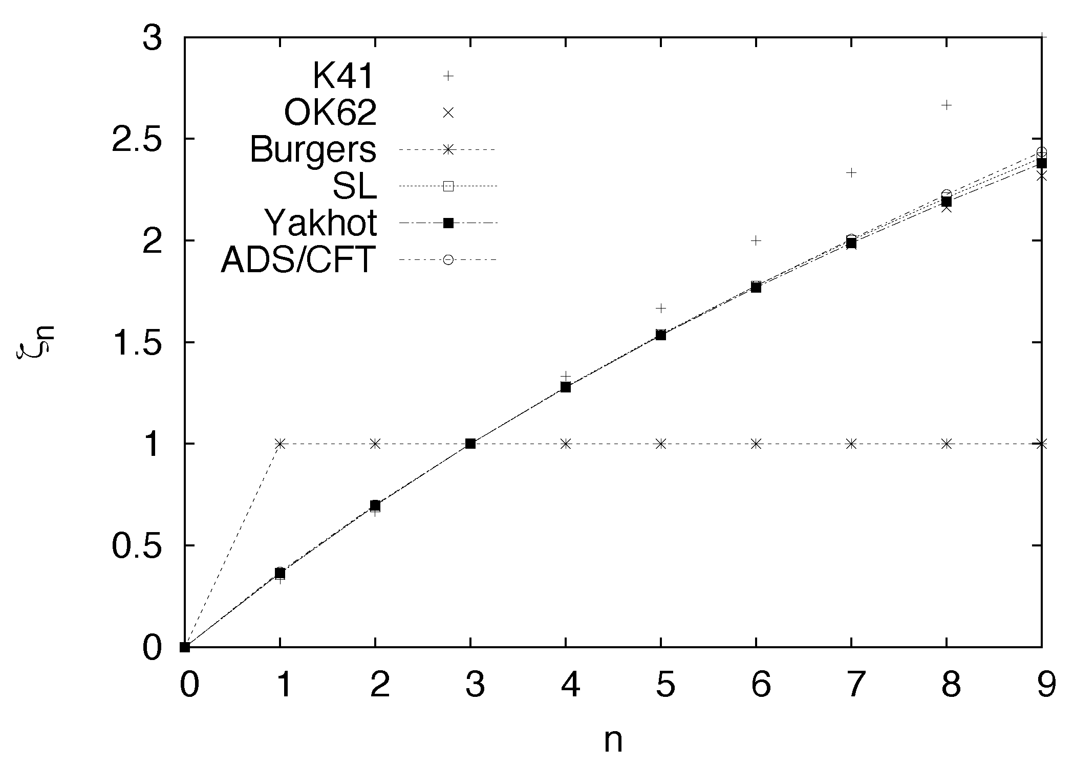
is general enough to capture the essence of anomalous scaling. In other words, all currently known phenomenological models of turbulence—characterized by their corresponding sets of scaling exponents ζ n as depicted in Figure 1—can be reproduced by the Kramers–Moyal expansion (7) with Kramers–Moyal coefficients (18) where reduced Kramers–Moyal coefficients K n are related to the scaling exponents ζ n by Equation (17). In the next subsections, we will describe in detail how these different phenomenological models can be mapped onto the Kramers–Moyal coefficients.
(i.) Kolmogorov’s theory K41:
The monofractal K41 phenomenology [3] states that ( δ r v ) n = C n ε n / 3 r n / 3 and an evaluation of the reduced Kramers–Moyal coefficients (17) suggests that it can be reproduced by just a single Kramers–Moyal coefficient
K n = { 1 / 3 for n 1 , 0 for n > 1 .
(ii.) Oboukhov–Kolmogorov theory OK62:
A first intermittency model which assumes a log-normal distribution of the local rate of energy dissipation ε has been proposed by Kolmogorov [4] and Oboukhov [5].
It predicts the scaling of the structure functions according to ( δ r v ) n = C n ε n 3 r n 3 r L n ( n 3 ) μ 18 where L is the integral length scale and μ is the so-called intermittency coefficient which is of the order μ 0.227 (recent experiments [26], however, suggest a value of μ = 0.17 ± 0.01 ). As it has been discussed by Friedrich and Peinke [8], this reduces the Kramers–Moyal expansion to a Fokker–Planck equation with drift and diffusion coefficient
K 1 = 3 + μ 9 and K 2 = μ 9 ,
and implies the vanishing of all higher-order coefficients.
(iii.) Burgers scaling:
The velocity structure functions in Burgers turbulence [19] follow the extreme scaling
( δ r v ) n = { C n ε n / 2 ν n / 2 r n for n < 1 , C n ε n 3 L n 3 1 r for n 1 .
Here, the first scaling is due to smooth positive velocity increments in the ramps, whereas the latter scaling corresponds to negative velocity increments dominated by shocks that form due to the compressibility of the velocity field in the vicinity of the viscosity ν 0 .
The smooth solutions correspond to a single Kramers–Moyal coefficient, whereas the shock solutions can only be reproduced by an infinite number of Kramers–Moyal coefficients and we obtain
K 1 = 1 , K n = 0 for n > 1 , for positive increments . K n = 1 , n for negative increments .
(iv.) She–Leveque model:
The She–Leveque model [6] for 3D Navier–Stokes turbulence predicts scaling exponents ζ n = n 9 + 2 1 2 3 n / 3 that are in very good agreement with both experimental and numerical data. This yields an infinite set of coefficients [27] and the reduced Kramers–Moyal coefficients read
K n = n 9 1 F 0 ( 1 n ; ; 1 ) + 2 1 2 3 3 n ,
where ν F n ( a ; b ; z ) is the generalized hypergeometric function. It has been shown recently [28] that this particular model can be apprehended as a jump process of a stochastic process for the velocity increments in scale.
(v.) Yakhot model:
Yakhot [29,30] introduced a model for structure function exponents ζ 2 n = 2 ( 1 + 3 β ) n 3 ( 1 + 2 β n ) based on a mean-field approximation. Similar scaling exponents were first derived by Novikov [31] and subsequently by Castaing [32]. With the choice of β = 0.05 , structure functions agree equally well with experimental data as the popular She–Leveque model. The translation to the Krames-Moyal coefficients is given by
K n = Γ [ n + 1 ] Γ n + 1 + 1 β Γ 1 + 1 β + 1 3 β 2 Γ 1 β .
(vi.) ADS/CFT random geometry model:
Eling and Oz [33] introduced a structure function scaling model which is motivated by a gravitational Knizhnik–Polyakov–Zamolodchikov (KPZ)-type relation. For 3D Navier–Stokes turbulence, they derive
ζ n = ( 1 + γ 2 ) 2 + 4 γ 2 ( n 3 1 ) 1 2 + γ 2 1 2 γ 2 ,
where experimental data suggest the value γ 2 = 0.161 . Unfortunately, we could not obtain an analytical formula for the coefficients of this particular model and have restricted ourselves to a numerical evaluation of Equation (17).
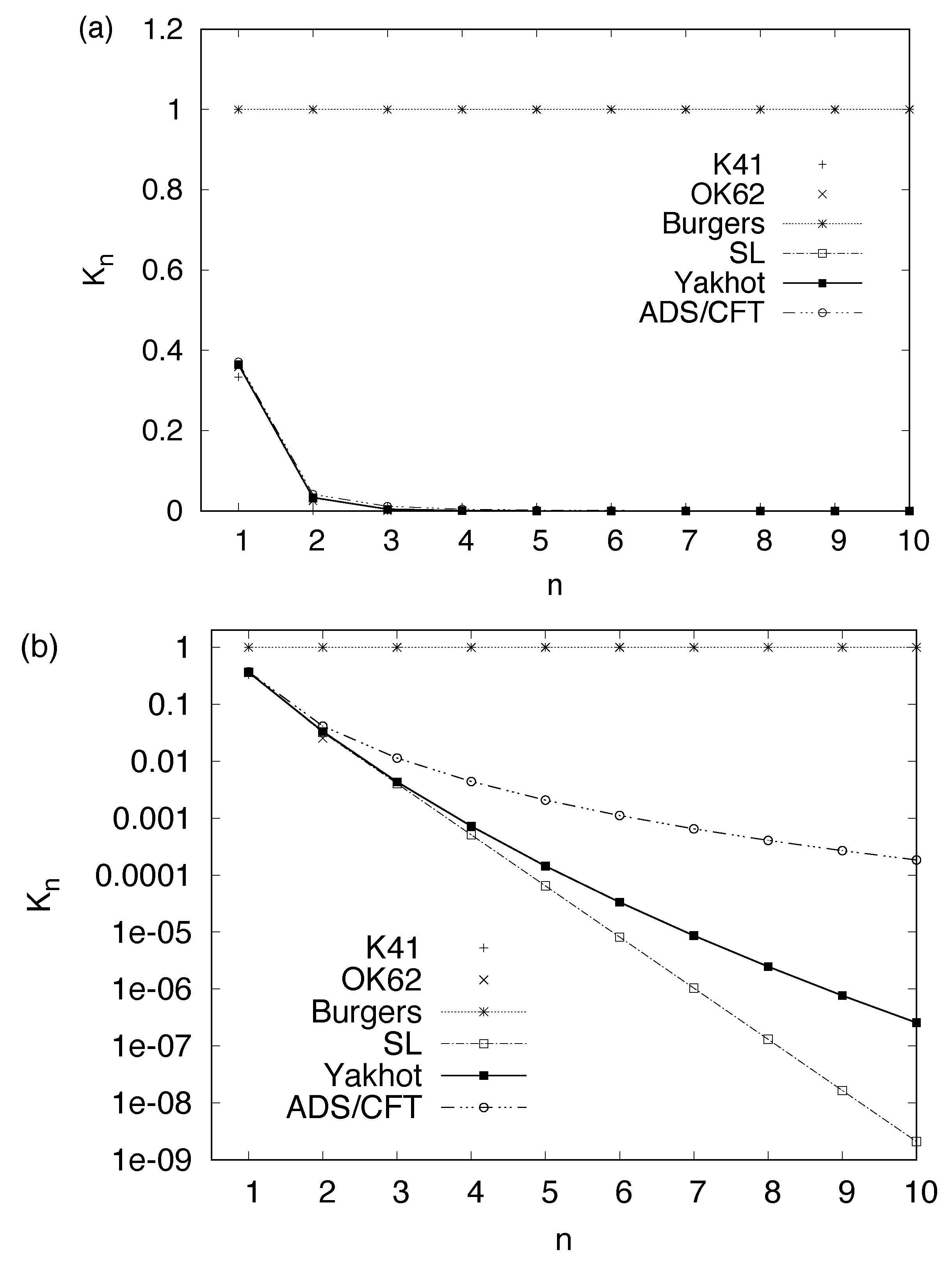
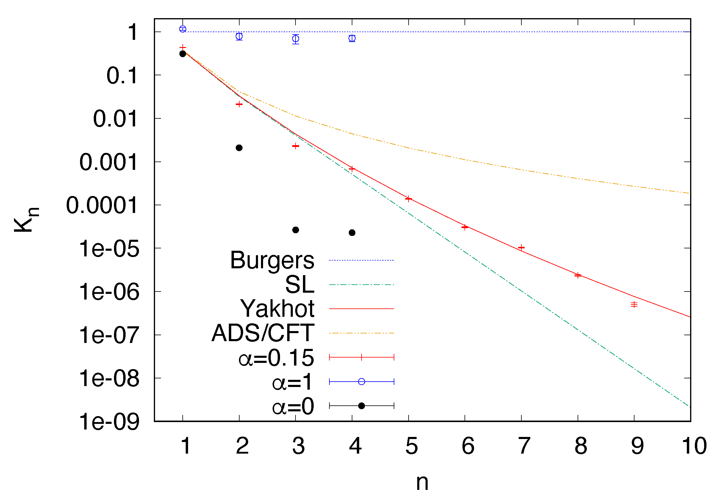
We have plotted the reduced Kramers–Moyal coefficients K n for the different models up to the order n = 10 in Figure 2a. As one can see, all models besides K41 and Burgers can hardly be distinguished from one another and the reduced Kramers–Moyal coefficients seem to tend towards zero very quickly. According to a theorem due to Pawula [34] (see also [25]), the vanishing of the fourth-order Kramers–Moyal coefficient implies that all higher coefficients are zero as well and the Kramers–Moyal expansion (7) reduces to an ordinary Fokker–Planck equation. The latter is particularly suitable for modeling approaches via its corresponding Langevin equation as well as the undemanding determination of statistical quantities via the exact short-scale propagator of the Fokker–Planck equation [25].
In the original work [8] and also all subsequent works [9,10,35], it was argued in favor of Pawula’s theorem since the experimentally determined Kramers–Moyal coefficient of order four was very close to zero. Figure 2a seems to agree qualitatively with this finding. However, in order to demonstrate that this can be misleading, we show a semi-logarithmic plot of Figure 2a in Figure 2b. It can be seen that the models (iv.)–(vi.) tend asymptotically towards zero and higher-order Kramers–Moyal are rather small but strictly non-zero. At this point, we want to emphasize that since K 4 10 3 , the significant detection of these higher-order coefficients in the experiment might be quite challenging due to the presence of measurement noise or insufficient statistics. Nevertheless, since the models (iv.)–(vi.) agree quite well with experimental data, an accurate determination of the higher-order coefficients should be within the reach of a spatially and temporarily well-resolved high-Reynolds number experiment. Moreover, Pawula’s theorem directly reduces the velocity increment statistics to families of the OK62 phenomenology (ii.). It should therefore be noted that the latter is only valid for moments v n that do not exceed the order n 3 2 + 3 μ , due to the convexity condition for ζ 2 n (see also [7] for further discussion). Consequently, one should bear in mind that, whilst modeling or other purposes of the Fokker–Planck approach, the tails of the PDFs might not be described accurately, although—admittedly—this effect should be rather small. In the following section, we want to quantify the small-scale intermittency behavior on the basis of the reduced Kramers–Moyal cofficients (17) at the example of a generalized Burgers equation with an additional nonlocality.

3. Direct Numerical Simulations of a Generalized Burgers Equation

We consider the generalized Burgers equation
t u ( x , t ) + α u ( x , t ) x u ( x , t ) + 1 α π p . v . d x u ( x , t ) x x x u ( x , t ) = ν 2 x 2 u ( x , t ) + F ( x , t ) ,
with forcing that is assumed to be white noise in time F ( x , t ) F ( x , t ) = χ ( x x ) δ ( t t ) . Here, the spatial correlation of the forcing follows a power law in Fourier space [36], namely
F ^ ( k , t ) F ^ ( k , t ) k 1 δ ( k k ) δ ( t t ) .
Moreover, α = 1 in Equation (26) corresponds to the case of Burgers turbulence, whereas α = 0 corresponds to a purely nonlocal case that is dominated by self-similar behavior [24]. The intermediate case α = 0.15 , however, exhibits several similarities to the intermittency behavior of 3D hydrodynamic turbulence. The latter manifest themselves by a skewed velocity gradient PDF, as well as by nonlinear scaling exponents ζ n of the velocity structure functions ( δ r v ) n | r | ζ n which has been reported by Zikanov, Thess, and Grauer [24]. Apparently, the balance between the nonlinear and nonlocal term results in particular dissipative structures that have considerable influence on the intermittency behavior of the system. Therefore, the model system (26) seems to be an interesting surrogate for the Navier–Stokes equation that allows for studying the competition between nonlinearity (steepening of velocity gradients) and nonlocality (regularization) in a systematic way, i.e., by controlling the parameter α (we also refer the reader to the monograph by Sagaut and Cambon [37] for a further discussion of these issues). It has to be stressed that, already due to the restriction to a single dimension in Equation (26), this cannot be considered as a one-to-one correspondence to 3D Navier–Stokes turbulence but rather corresponds to a model system with similar properties (non-self-similarity of the velocity increment PDF, skewness).
Equation (26) has been solved with the help of a standard pseudo-spectral code. A third order Runge–Kutta method was used for the time stepping due to its vigor of capturing the temporal evolution of shock-like structures [38]. Furthermore, aliasing errors that occur due to an insufficient resolution of the quadratic nonlinearities were treated with the help of a filter in Fourier space [39]. Concerning the realization of the forcing determined by Equation (27), we assured the white-noise in time condition with a numerical method for the Langevin equation discussed by Higham [40]. Cheklov and Yakhot [36] reported that a power law correlation function k 1 results in a Kolmogorov-type spectrum which can also be determined on the basis of a one-loop renormalization group consideration. Here, the nonlinearity directly balances forcing contributions that are acting on all scales. Therefore, the cut-off of the forcing is located in the neighborhood of the dissipation range in all simulations.
Table 1 shows the characteristic parameters of the DNS. The attained Reynolds numbers in the simulations are not as high as the Reynolds numbers attained in references [24,36]. This is due to the fact that the latter results were obtained with a so-called hyperviscous term, i.e., replacing 2 x 2 by 2 α x 2 α , which leads to an efficient damping of the higher wavenumber (small-scale) components of the velocity field. By this method, higher Reynolds numbers can be attained, which leads to an increased inertial range. Apparently, the concept of hyperviscosity has no considerable influence on the inertial range behavior [36]; therefore, it can be considered as an efficient method to attain higher Reynolds numbers. Nonetheless, in this work, we intend to investigate the original dissipative effects, and thus only the Laplacian viscous term has been considered. Moreover, we chose the resolution N in a way which allows for the production of a sufficient amount of data. These restrictions lead to the moderate Reynolds numbers in Table 1.

3.1. Strong Intermittency α = 1 : Burgers Equation

For the case α = 1 , the additional nonlocality in Equation (
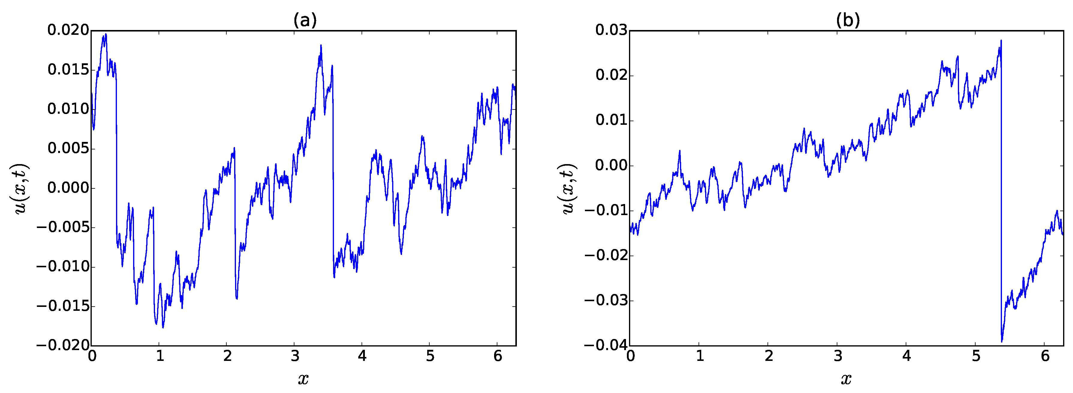
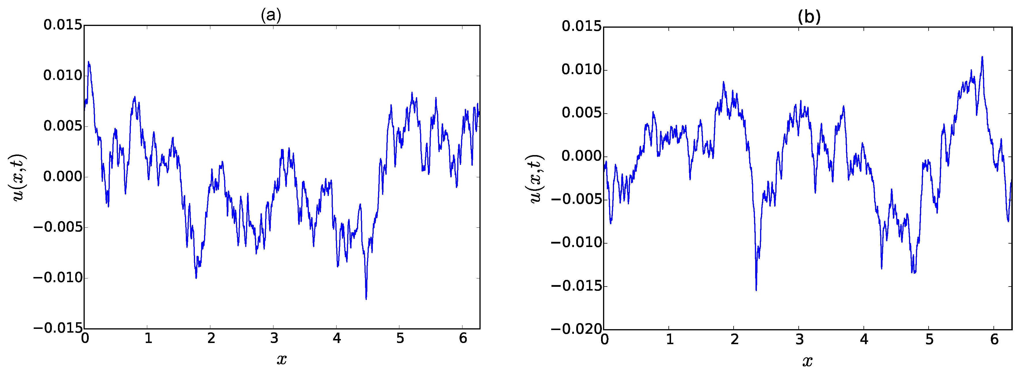
26) vanishes and we recover the ordinary Burgers equation with its shock-type velocity profiles. A typical realization of the velocity field of Burgers turbulence (run #1) is shown in Figure 3a. The velocity field exhibits a sawtooth-like structure and forms shock fronts consisting of large negative velocity gradients. In this particular snapshot, we can distinguish three or four shocks that are connected via ramps of positive inclination and are superimposed by small-scale structures that also consist of small shocks. Figure 3b shows the velocity field belonging to the most extreme shock event that occurred during the simulations. It consists of one large negative gradient event that is barely resolved by the corresponding resolution of N = 3072 grid points. Events such as the one depicted in Figure 3b are extremely rare, but they do bear a particular statistical significance.
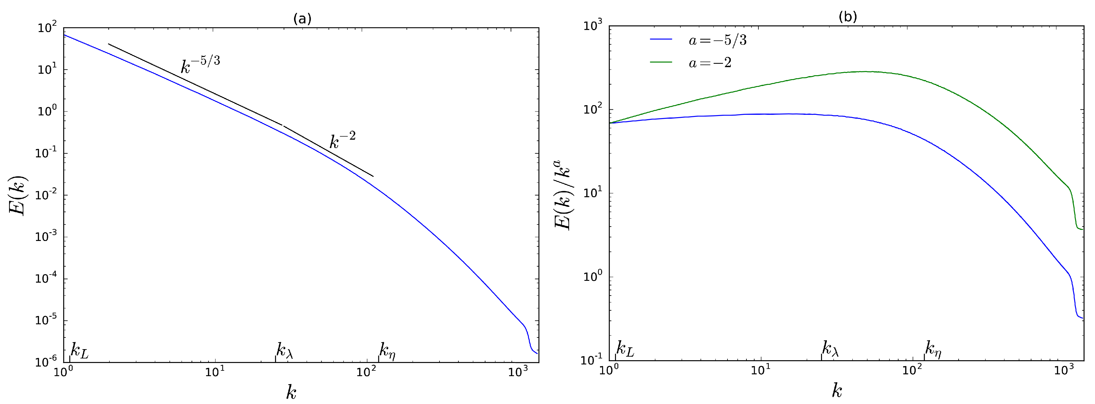
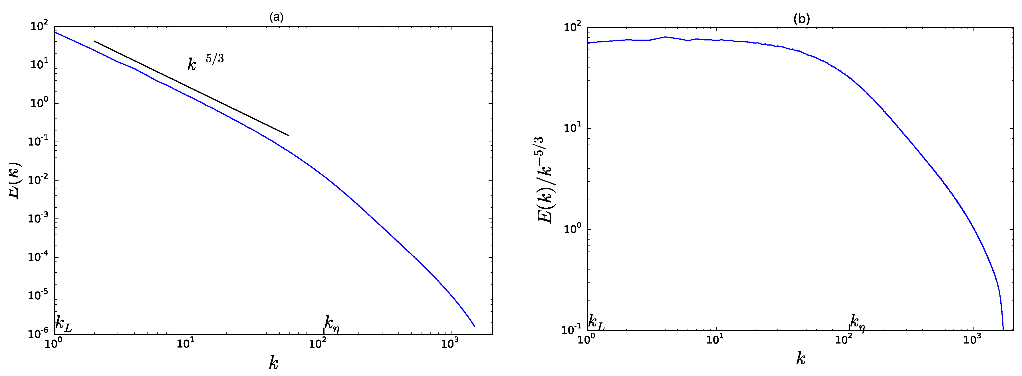
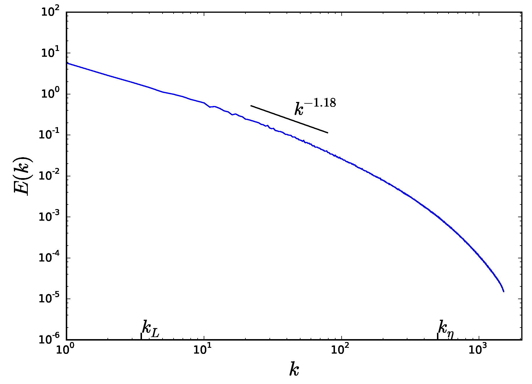
Figure 4a shows the energy spectrum E ( k ) of simulation #1. Here, the inertial range is limited by the wave numbers k L and k η which are associated with the integral length scale L and the Kolmogorov dissipation length η . The small wavenumber regime can be described quite accurately by a Kolmogorov-like spectrum E ( k ) k 5 / 3 . However, as the wavenumbers increase, the spectrum drops faster than the Kolmogorov spectrum. It is tempting to propose a shock-like spectrum E ( k ) k 2 for intermediate wavenumbers 60 < k < 80 that piles up in front of the dissipation range. Obviously, the latter does not manifest itself as clear as the k 5 / 3 -part, but since the spectrum drops already in front of the dissipation range and shocks represent a small-scale quantity, it seems to be a convenient explanation. We must emphasize, however, that, in the original work of Cheklov and Yakhot [36], solely the Kolmogorov-spectrum has been observed. The latter finding might be a result of hyperviscosity and the attained high Reynolds numbers. In order to further quantify these tendencies, Figure 4b shows compensated spectra E ( k ) / k a with a = 5 / 3 and a = 2 . Plateaus in the plot correspond to scaling behavior of the spectrum and confirm the Kolmogorov part at small wavenumbers and a small range of the shock-like part as well.
Figure 5 shows the evolution of the one-increment PDF f 1 ( v , r ) in scale, where r is expressed in multiples of the Taylor length λ . At small scales, the PDF shows a pronounced left tail due to shock events, whereas it is close to Gaussian on large scales. Here, the PDF for r = 0.3 λ seems to exhibit an algebraic part for negative increments and drops exponentially for larger negative increments. However, it is not obvious whether the algebraic part corresponds to ( v / r ) 7 / 2 as it has been predicted for the gradient PDF [15]. Due to the moderate Reynolds numbers, it is also not clear whether the exponential decay for large negative velocity increments follows the exponential decay e v / ( Re r ) ) 3 / 2 predicted from instanton calculations [41].

3.1.1. Examination of the Markov Property

In this section, we seek to examine the Markov property (4) from DNS of Burgers turbulence. To this end, we briefly mention two possibilities: first, the Markov property can be examined directly in comparing the conditioned PDF with the transition PDF
p ( v 3 , L / 2 Δ r | v 2 , L / 2 ; v 1 , L / 2 + Δ r ) = p ( v 3 , L / 2 Δ r | v 2 , L / 2 ) ,
where the intermediate scale L / 2 was chosen to lie well within the inertial range and Δ r can be considered as the variable step width of the process. In general, the intermediate scale can also be chosen at a different inertial range scale, but in the following we will only consider this particular case. At this point, since we are comparing two objects of different complexity, we perform cuts of the doubly conditioned PDF for fixed v 1 . This can be done by the simple choice v 1 = 0 , which offers the best statistics. However, for a more critical examination, it is appropriate to put v 1 at least to σ , where
σ = lim r ( δ r v ) 2 = lim r ( u ( R + r ) u ( R ) ) 2 = 2 u r m s .
The other method is to examine the Chapman–Kolmogorov equation [25]
d v 2 p ( v 3 , L / 2 Δ r | v 2 , L / 2 ) p ( v 2 , L / 2 | v 1 , L / 2 + Δ r ) = p ( v 3 , L / 2 Δ r | v 1 , L / 2 + Δ r ) ,
which has the advantage that it involves solely transition PDFs.
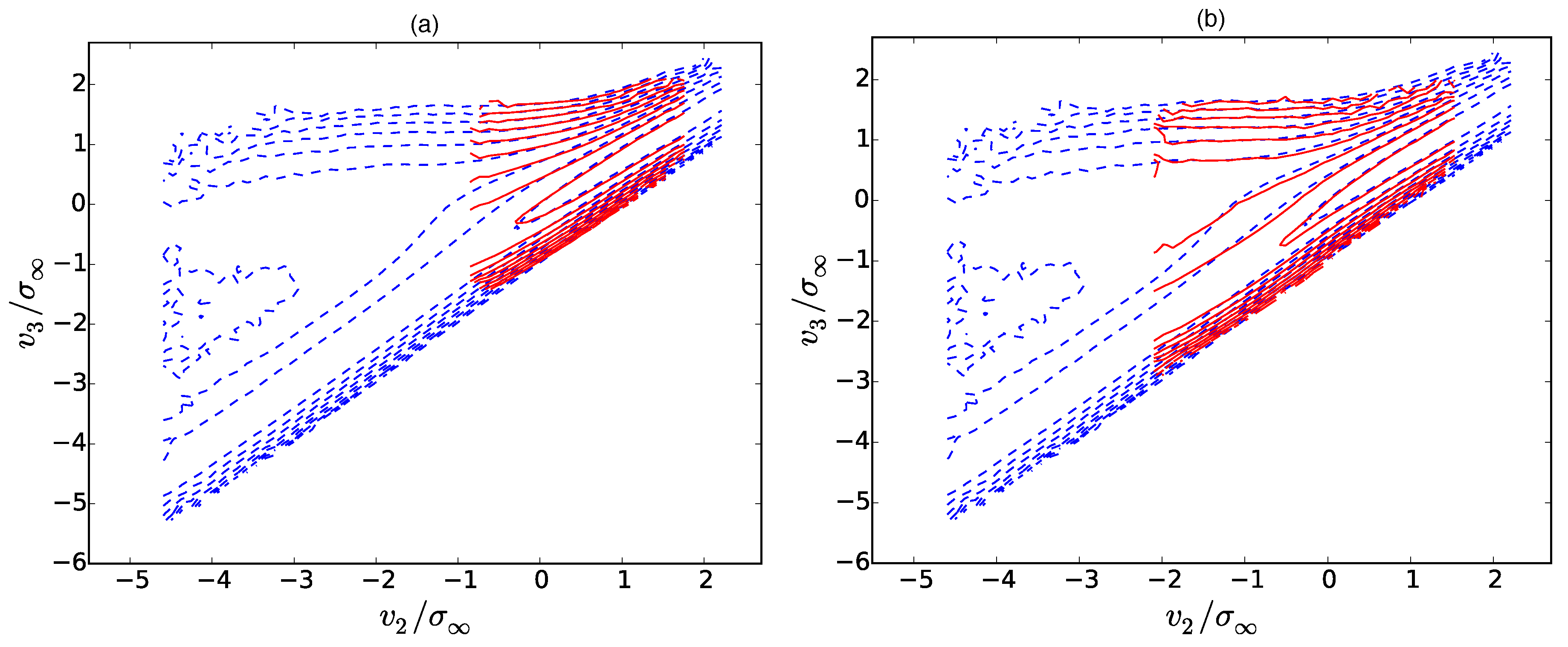
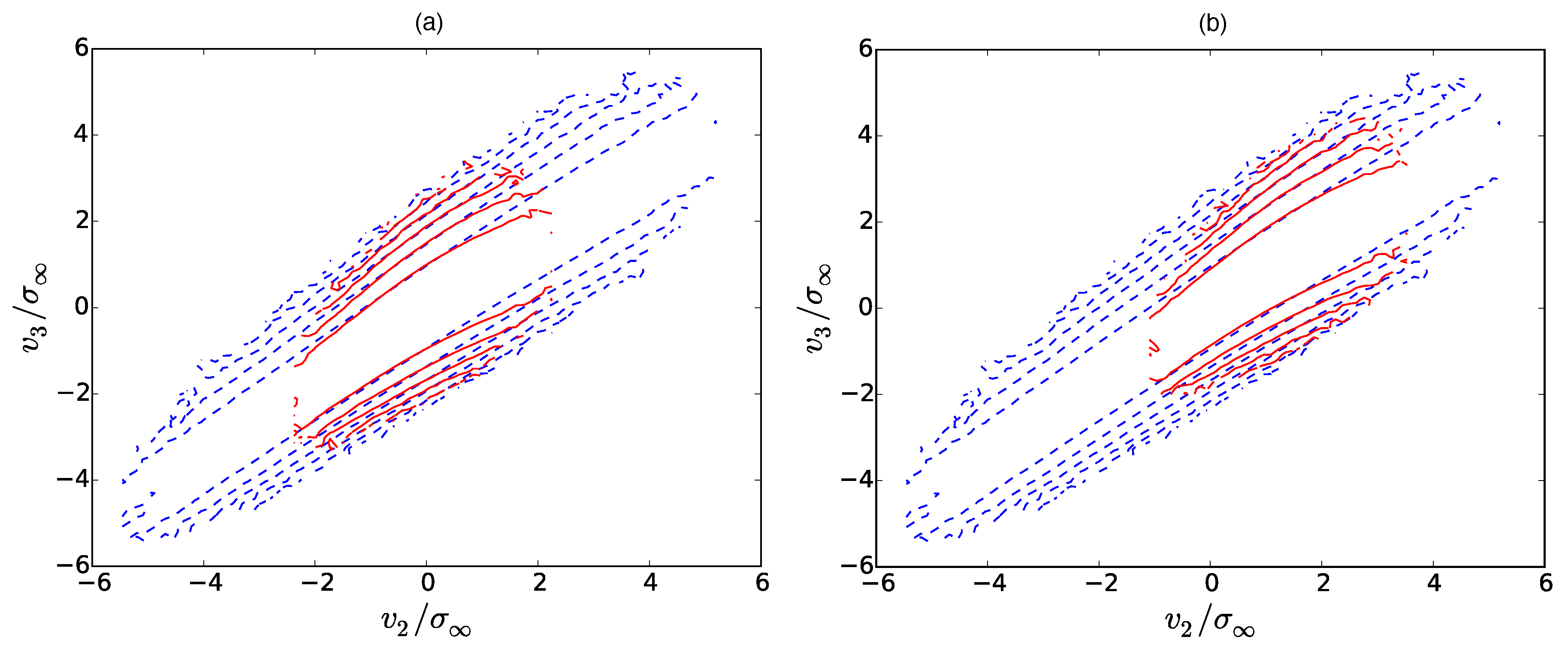
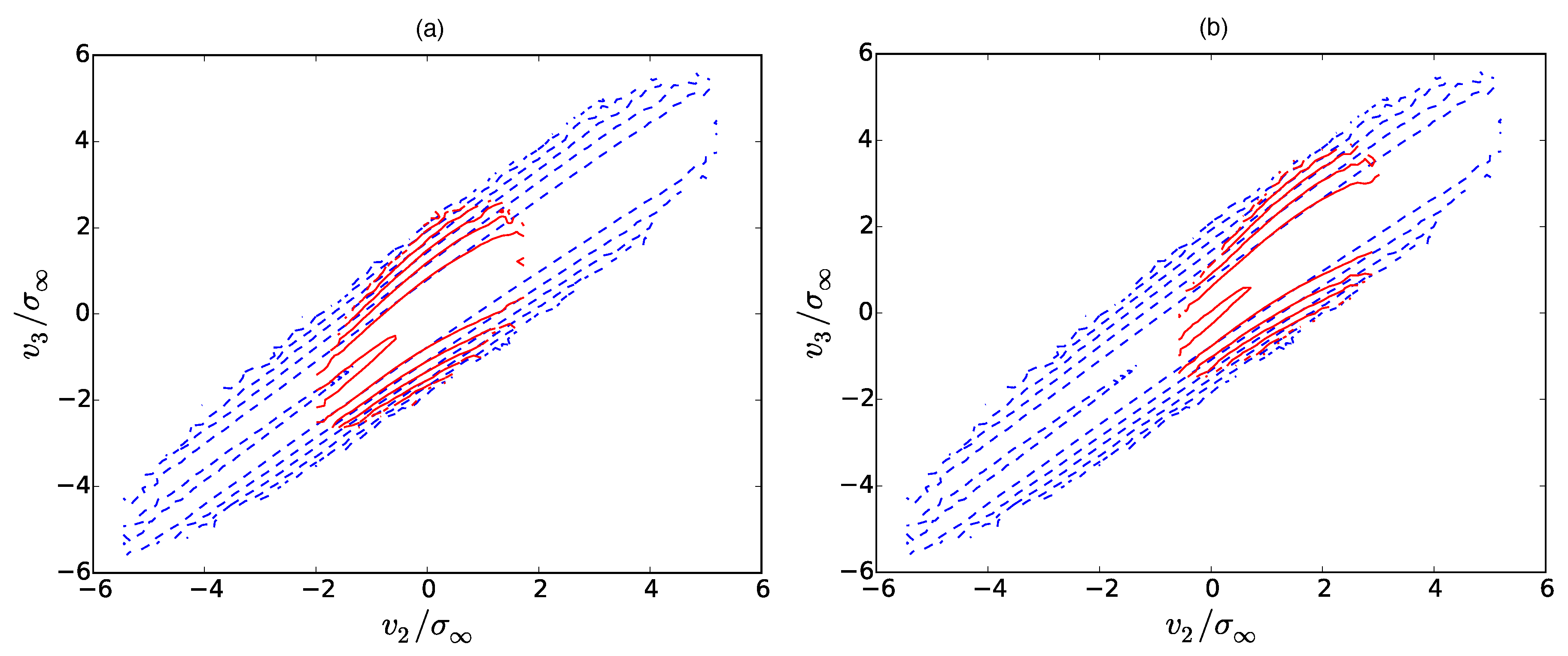
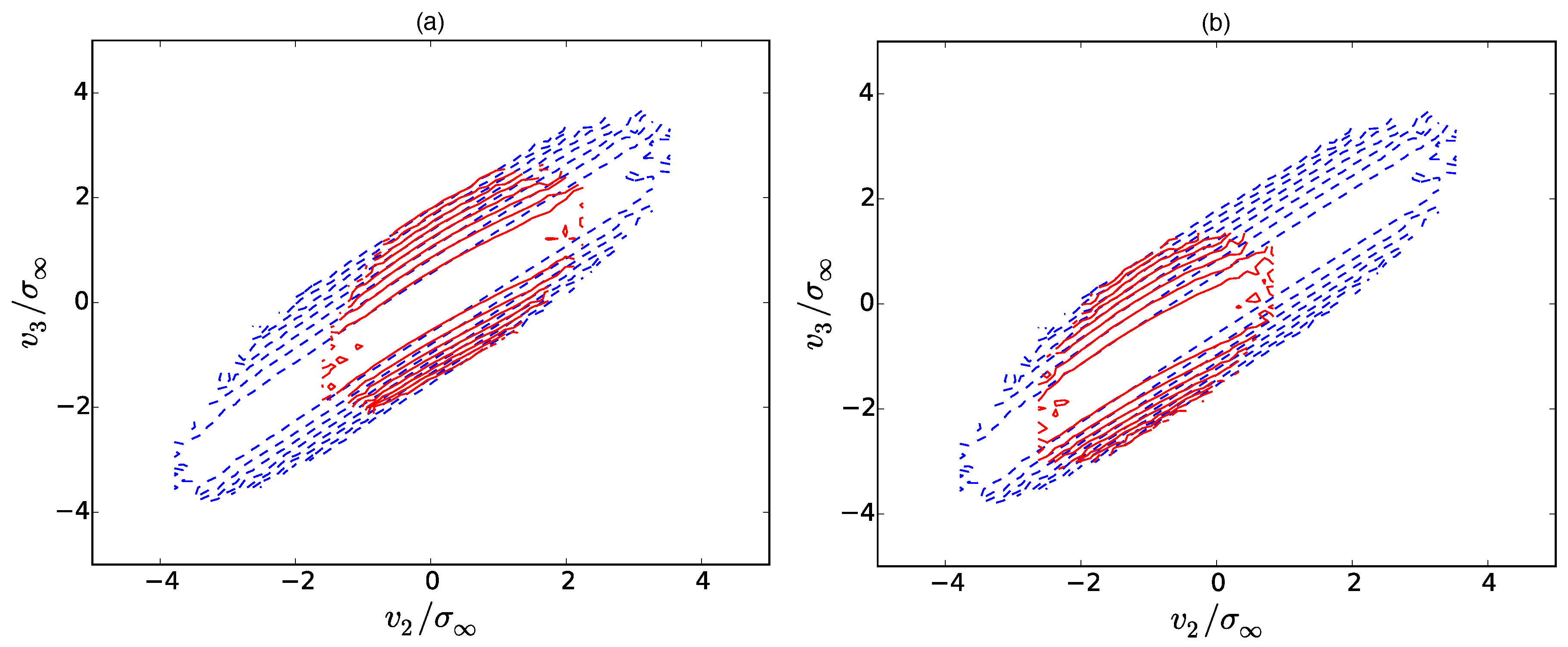
In the following, we use the first method, i.e., Equation (28). In order to obtain a sufficient overlap between the two PDFs, we choose v 1 = 0 and v 1 = 1 σ , since the positive increment parts of the PDFs are suppressed by shocks. The resulting contour plots for three different Δ r are depicted in Figure 6, Figure 7 and Figure 8. Here, the dashed blue lines correspond to the transition PDF p ( v 3 , L / 2 Δ r | v 2 , L / 2 ) , whereas the red lines correspond to the conditional PDF p ( v 3 , L / 2 Δ r | v 2 , L / 2 ; v 1 , L / 2 + Δ r ) . At first glance, we can see that the shape of the transition PDF (blue) can be reproduced for the most part by the solution of (8)
p ( v 3 , r 3 | v 2 , r 2 ) = δ v 3 r 3 r 2 v 2 for v 2 0 , r 3 r 2 δ ( v 3 v 2 ) + 1 r 3 r 2 δ ( v 3 ) for v 2 0 . ,
which is derived in Appendix A. For v 2 < 0 , the additional branch δ ( v 3 ) appears. Obviously, the contours of the transition PDFs are not pure delta functions, but are rather broad. We want to emphasize that this can be considered as an artifact of the Kramers–Moyal expansion (8): The solution (31) has been constructed from the initial condition
lim r 3 r 2 p ( v 3 , r 3 | v 2 , r 2 ) = δ ( v 3 v 2 ) .
A second initial condition, which would be a Gaussian transition probability at large scales, cannot be imposed since the Kramers–Moyal expansion is only a first-order differential equation.
The overall structure in Figure 6, Figure 7 and Figure 8, however, agrees fairly well with the theoretical predictions (31).
Concerning the Markov property itself, it seems to be best fulfilled around the Taylor length, i.e., for Δ r = 1 λ in Figure 7a. We can also establish this finding for v 1 = σ . However, at larger scale separations Δ r = 2 λ in Figure 6, the Markov property slightly deteriorates. Although the shape of the transition PDF and the conditional PDF are basically the same, there is a small shift of the contour lines in the v 3 -direction. The effect becomes even stronger for v 1 = σ which can be seen from 
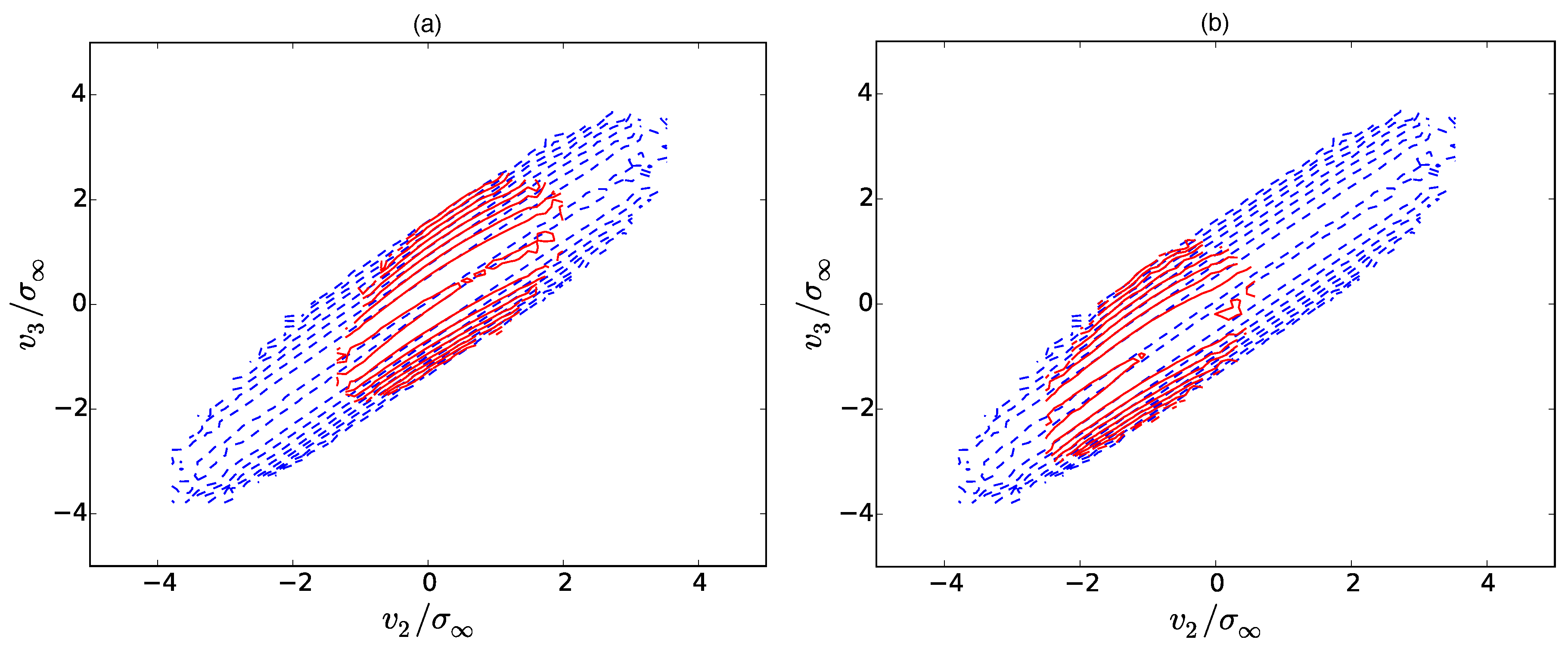
Figure 6b. In comparison to the true violation of the Markov property in Figure 8, however, this effect is rather small. At those smaller scale separations, here for Δ r = 0.1 λ , both PDFs possess a different shape. Figure 8a shows that the transition PDF (red) overestimates the v 3 v 2 -correlations of the conditional PDF (blue) manifesting itself by a strong steepening of the contour lines of the transition PDF in comparison to the conditional PDF. The effect becomes even more pronounced for v 1 = σ . Nevertheless, for large negative values v 2 , the contour lines seem to overlap again. It is therefore tempting to speculate about whether the Markov property might again be fulfilled inside the shocks, and that only the regions of extreme curvature in the vicinity of the shocks lead to the break-down of the Markov property. In this context, it is important to notice that the Taylor length λ is located just in front of the k 2 -part of the spectrum in Figure 4. In the following section, we aim to quantify the break-down of the Markov property by the introduction of a distance measure between the two distributions in Equation (28).

3.1.2. Determination of the Markov–Einstein Length

Here, we seek to quantify the break-down of the Markov property (28). There are a variety of methods for comparing the transition PDF and the conditional PDF [10]. In the present study, we will restrict ourselves to the so-called Hellinger distance [42], although other methods such as the correlation distance or the Kullback–Leibler divergence have also been experimented with. The advantage of the Hellinger distance H is that it forms a true metric in the space of the PDFs and can therefore be used to decide at which scale separation Δ r the Markov property significantly deteriorates. The Hellinger distance H for continuous distributions is defined according to
H 2 ( v 2 , v 1 ; Δ r ) = 1 2 d v 3 p ( v 3 , L / 2 Δ r | v 2 , L / 2 ; v 1 , L / 2 + Δ r ) p ( v 3 , L / 2 Δ r | v 2 , L / 2 ) 2 = 1 d v 3 p ( v 3 , L / 2 Δ r | v 2 , L / 2 ; v 1 , L / 2 + Δ r ) p ( v 3 , L / 2 Δ r | v 2 , L / 2 ) .
Here, we made use of the identities
d v 3 p ( v 3 , L / 2 Δ r | v 2 , L / 2 ; v 1 , L / 2 + Δ r ) = 1 and d v 3 p ( v 3 , L / 2 Δ r | v 2 , L / 2 ) = 1 ,
in the last step. Hence, the Hellinger distance is symmetric in both probabilities and is restricted to
0 H ( v 2 , v 1 ; Δ r ) 1 ,
which is a direct consequence of the Cauchy–Schwarz inequality. Another useful property of the Hellinger distance is that it can be explicitly calculated for certain types of PDFs (normal distribution, beta distribution, exponential distribution, etc.).
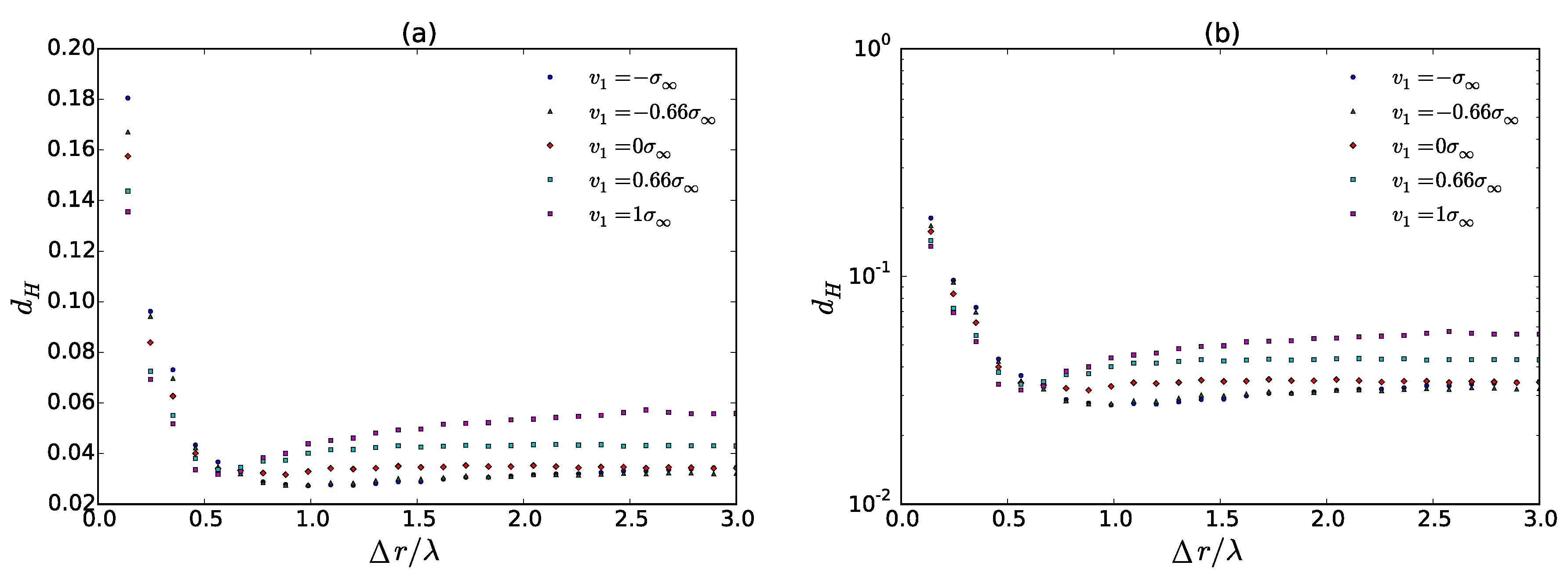
In our case, the Hellinger distance still is a function of v 2 if we assume that v 1 is fixed. Therefore, an average of the corresponding v 2 -values is performed in order to obtain a pure correlation measure
d H ( Δ r , v 1 ) = H ( v 2 , v 1 ; Δ r ) v 2 .
The corresponding Δ r dependency in Figure 9a is expressed in terms of the Taylor length λ . Remarkably, the Hellinger distance d H ( Δ r ) is smallest at around Δ r = λ and approaches a small constant that is different from zero for larger Δ r . This corresponds to the observation from Figure 6 where the contour plots were slightly shifted in the v 3 -direction for larger Δ r . In other words, the Markov property gets slightly better before it gets worse in the process of letting Δ r 0 . The latter observation differs from usual investigations of the Markov property in turbulence [10]. For smaller Δ r < 0.8 λ , however, the Hellinger distance shows a more pronounced increase and therefore, the Markov property is clearly violated since it seems to approach 1 in the limit r 0 . These effects become even more unambiguous for v 1 = 0.33 σ , 0.66 σ , σ . Figure 9b shows a semi-logarithmic plot of the Hellinger distance. For Δ r < 0.8 λ , a quantitatively new behavior emerges. The latter is characterized by a close to exponential increase of the Hellinger distance. Such behavior implies an exponential decay of the correlations of the Markov property Equation (28). Here, it suffices to estimate the Einstein–Markov length at around the point, where a pronounced increase sets in, i.e., λ M E = 0.8 λ .
Hence, the task of an accurate determination of the Markov–Einstein length is far from obvious. However, it can be inferred from Figure 9 that it lies near the Taylor length as the correlation measure clearly drops at Δ r / λ 1 .

3.1.3. Determination of the Kramers–Moyal Coefficients

In this section, we will outline a procedure which determines the Kramers–Moyal coefficients (10) from the numerically evaluated transition probabilities similar to Figure 7.
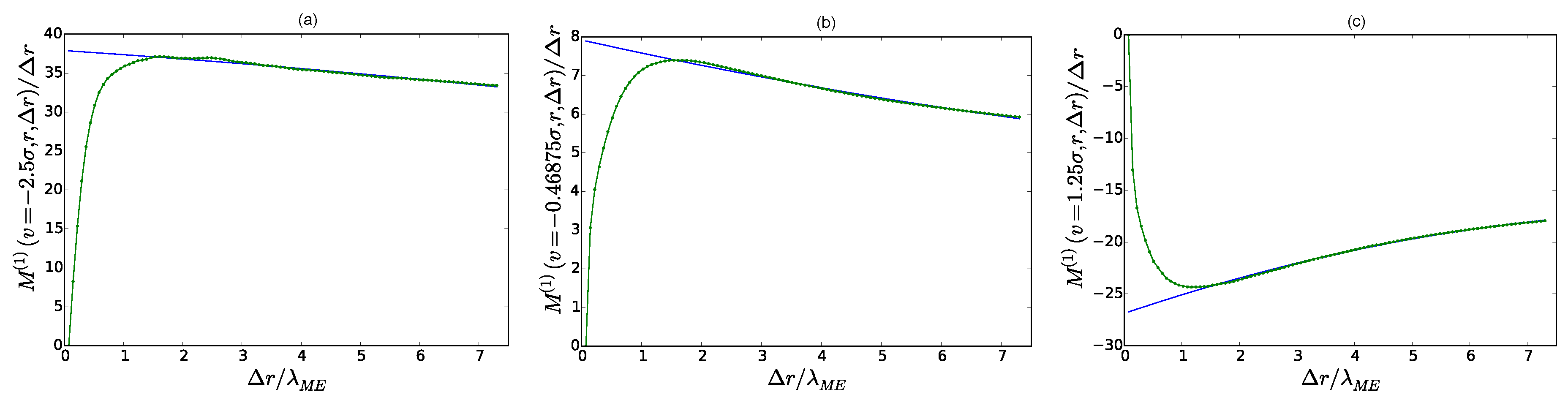
To this end, we devise an appropriate extrapolation method for the conditional moments
M ( n ) ( v , r ; Δ r ) = d v ( v v ) n p ( v , r Δ r | v , r ) ,
as the Markov property becomes violated in the proximity of the Einstein–Markov length. Subsequently, the limit
lim Δ r 0 M ( n ) ( v , r ; Δ r ) Δ r = D ( n ) ( v , r ) ,
has to be determined from the extrapolation of the conditional moments in order to obtain the corresponding Kramers–Moyal coefficient [10]. As an example, we plotted the conditional moments of first order M ( 1 ) ( v , r ; Δ r ) Δ r for three different v 1 in Figure 10. M ( 1 ) ( v , r ; Δ r ) / Δ r drops against zero for Δ r < λ M E as the Markov property is violated. In order to extrapolate the moments, polynomial fits of second order in Δ r were performed for Δ r > λ M E (blue lines in the plots). The Kramers–Moyal coefficient for a particular v, in this case the drift coefficient, can be read off from the y-intercepts of the fits. Consequently, this procedure has to be repeated for several v (and in general also different r) for the sake of obtaining the full functional form of the Kramers–Moyal coefficients. The method was used for the Kramers–Moyal coefficients up to order four in Figure 11. The corresponding coefficients were fitted with polynomials of order n. The obtained reduced Kramers–Moyal coefficients K n correspond well with the theoretical predictions from Equation (22) even at such small Reynolds numbers. Kramers–Moyal coefficients of higher order are detectable for negative velocity increments and Pawula’s theorem [34] is violated. The drift coefficient D ( n ) ( v , r ) possesses an additional cubic v-dependence that has already been reported in the experiment [10]. In the Burgers case, only the drift coefficient is different from zero for positive increments, which underlines the self-similarity of the right tail of the PDF in Figure 5. The diffusion coefficient, however, possesses an additional positive intercept which turns out to be a consequence of the non-conservative forcing procedure. In fact, it can be shown that a conservative force F ( x , t ) in Equation (26) leads to the vanishing of the intercept.

3.2. No Intermittency α = 0 : Purely Nonlocal Case

In the following, we will discuss the purely nonlocal case ( α = 0 ) of the generalized Burgers Equation (26). Figure 12a shows a typical velocity field realization of the DNS of run #2 in Table 1. In contrast to the case of Burgers turbulence, no clear shock fronts can be detected and the velocity field is organized in cusp-like structures.
Apparently, the nonlocality in the generalized Burgers Equation (26) leads to entirely different singular structures. The latter manifest themselves also in the spectrum E ( k ) in Figure 13 which exhibits a close to Kolmogorov-type inertial range.

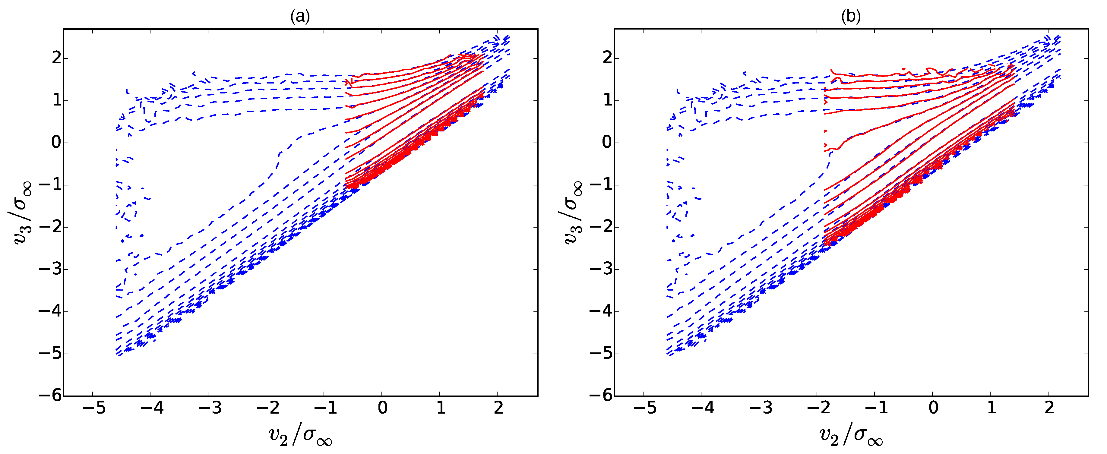
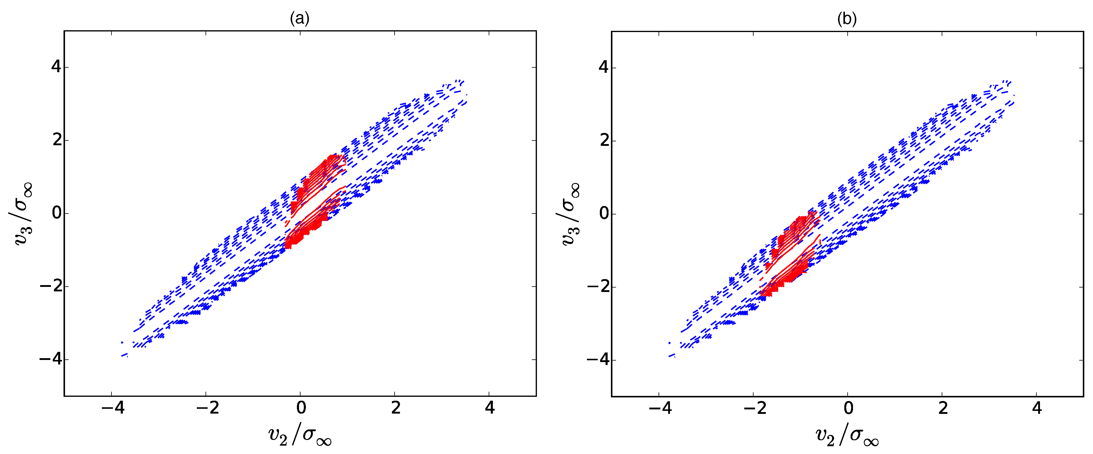
3.2.1. Examination of the Markov Property
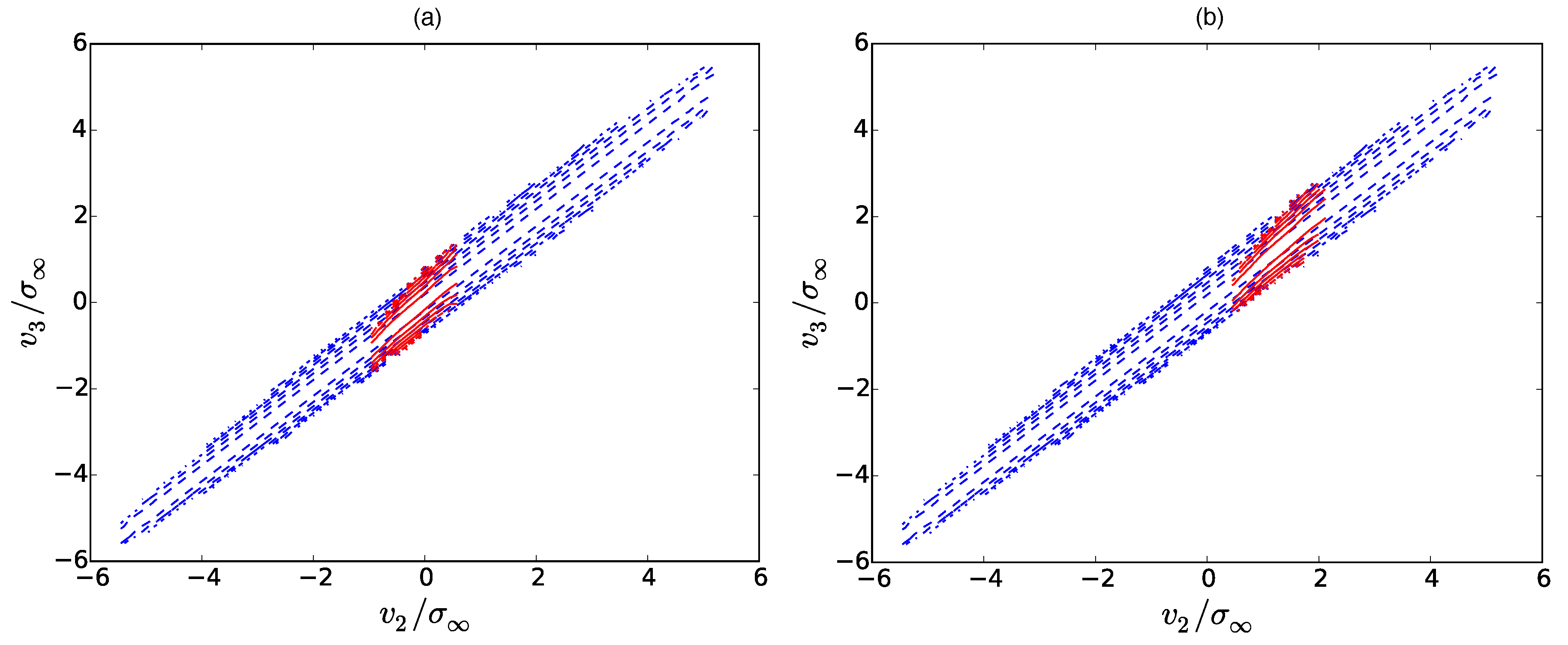
Figure 14, Figure 15 and Figure 16 show the contour plots of the one-time conditioned PDF (blue) and the two-time conditioned PDF (red). For this particular case, the transition PDF (blue) possesses a solely diagonal shape in contrast to the pure Burgers case in Section 3.1.1, which possessed a δ ( v 3 ) -part for negative v 2 .
The Markov property is fulfilled to a great extend for Δ r = 2.2 λ and Δ r = 1 λ in Figure 14 and Figure 15. For smaller scale separations, i.e., Δ r = 0.2 λ in Figure 16, the Markov property is broken: the doubly conditional PDF (red) appears steeper than the transition PDF (blue), which underestimates the correlations between v 3 and v 2 . The contours are shown for two different slices of p ( v 3 , L / 2 Δ r | v 2 , L / 2 ; v 1 , L / 2 Δ r ) , namely v 1 = 0 in (a) and v 1 = 1 σ . Contrary to the Burgers case in Figure 6, Figure 7 and Figure 8, the exact v 1 -position of the slice is quite unimportant and only alters the significant statistics, not the shape of the PDFs. For comparison, we also refer to Appendix B for an explicit solution for the K41 transition probability.

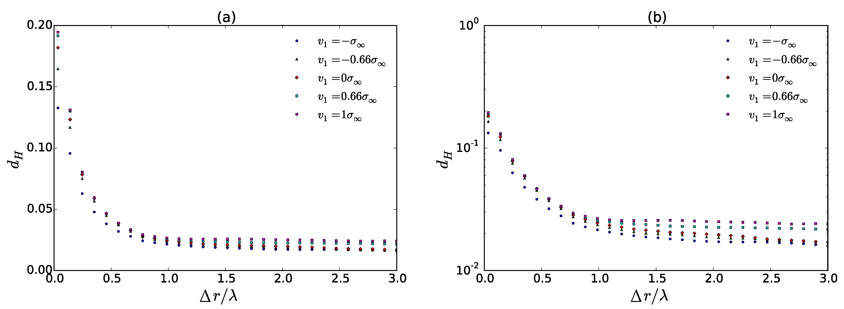
3.2.2. Determination of the Markov–Einstein Length

Figure 17 presents the Hellinger distance d H ( Δ r ) from Equation (36) for the purely nonlocal case. The Hellinger distance is close to zero for large scale separations Δ r . In contrast to the Burgers case in Figure 9, which exhibited a clear drop of the Hellinger distance at around Δ r = λ , the Markov property is a good approximation for all larger scale separations.
Here, the Hellinger distances increase at around Δ r = λ . It must be stressed that this behavior differs significantly from the Burgers case: whereas the Hellinger distances in Figure 9 decrease at around Δ r λ and then increase, i.e., they exhibit a clear minimum, the nonlocal case exhibits a steady increase at these scales. Figure 17b shows a semi-logarithmic plot of the Hellinger distance d H ( Δ r ) . Whether the increase of the Hellinger distance is exponential is somewhat hard to anticipate. However, the increase is not as violent as in the Burgers case in Figure 9b. Accordingly, the Markov property in the nonlocal case is not deteriorating as fast as in the Burgers case. The determination of the Markov–Einstein length λ M E for the nonlocal case proves to be quite challenging since the Hellinger distance is steadily increasing for smaller Δ r . In the following, we estimate λ M E = λ , in order to determine the Kramers–Moyal coefficients of the nonlocal case.

3.2.3. Determination of the Kramers–Moyal Coefficients
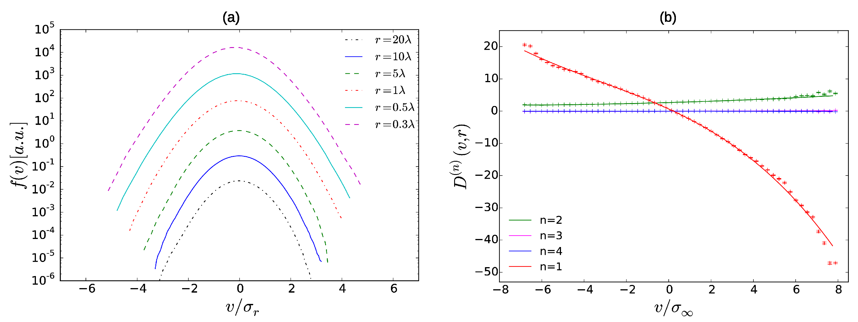
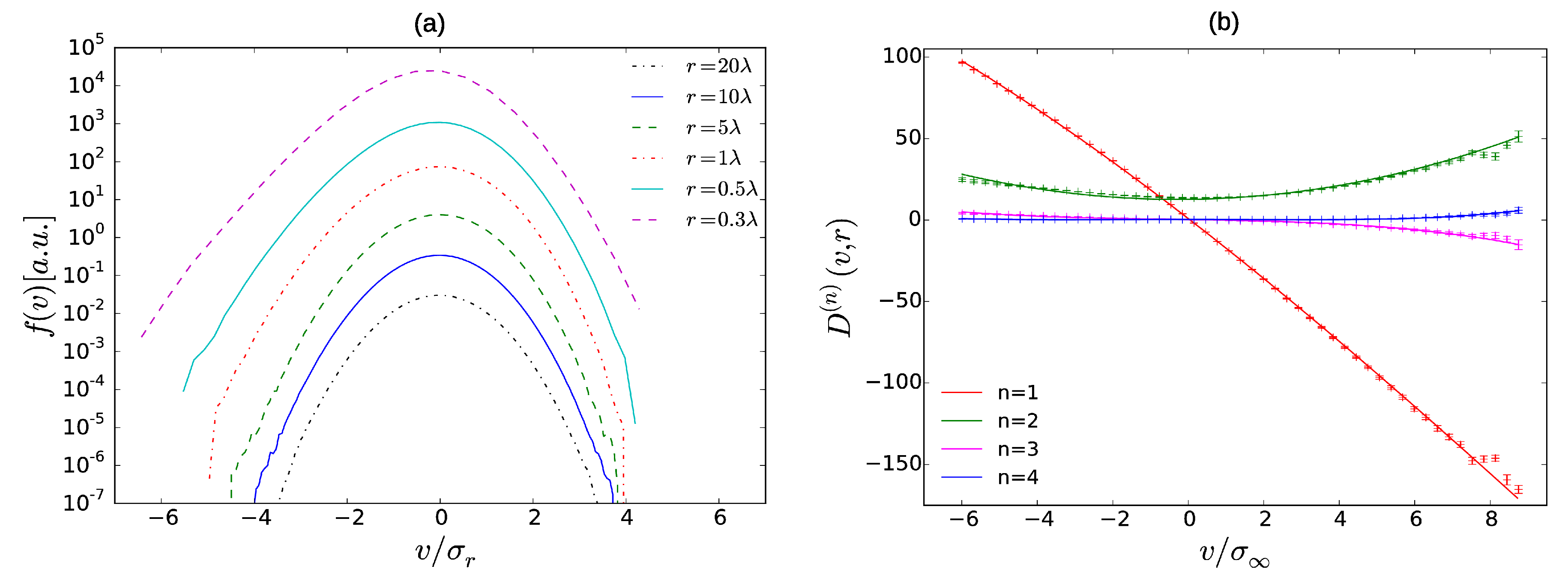
The PDFs f 1 ( v , r ) at different scales r in Figure 18a are purely self-similar functions that are close to Gaussian. Hence, the purely nonlocal case is characterized by the absence of intermittency. The self-similarity of the one-increment PDF is in agreement with the heuristic arguments established in Section 2 (i.). They can be reproduced by a self-similar function
f 1 ( v , r ) = 1 ( ε r ) α g v ( ε r ) α ,
with α 0.31 and g being very close to a Gaussian (not depicted in the figure). Hence, the nonlocal case is in very close correspondence to the K41 phenomenology. This is also reflected in the Kramers-Moyal coefficients depicted in Figure 18b. Whereas the drift coefficient D ( 1 ) ( v , r ) possesses a slightly cubic dependence, the linear part with its corresponding reduced Kramers–Moyal coefficient K 1 = 0.3108 ± 0.0002 is close to the K41 prediction K 1 = 1 / 3 . The diffusion coefficient points further into the direction of the K41 phenomenology: it shows only a slight quadratic dependence on v and has a rather linear shape. Accordingly, the reduced Kramers–Moyal coefficient of order two is rather small, K 2 = 0.0021 ± 0.0001 . Higher-order coefficients, n = 3 , 4 are even smaller ( K 3 = ( 2.64 ± 0.01 ) × 10 5 , K 4 = ( 2.28 ± 2.56 ) × 10 5 ). Furthermore, for n > 4 , the coefficients strongly deviate from the scaling D ( n ) ( v , r ) v n / r , e.g., the reduced Kramers–Moyal coefficients become negative. Hence, the obtained Kramers–Moyal coefficients are in agreement with the self-similarity of the one-increment PDF in Figure 18a.

3.3. Intermediate Case α = 0.15

Seminal numerical investigations [24] already highlighted the fact that the intermediate case exhibits statistical behavior that is close to the intermittency behavior encountered in ordinary hydrodynamic turbulence. The latter behavior manifested itself by a skewed velocity gradient PDF as well as by structure function exponents that deviated considerably from the predictions suggested by the K41 theory.
Figure 19a shows a snapshot of the velocity field obtained from DNS run #3. In contrast to run #2 in Figure 12, the intermediate case reveals a rather saw-tooth like velocity field profile. Nonetheless, no clear shock-like structures can be distinguished.
Figure 20 shows the energy spectrum of run #2. It deviates considerably from the Kolmogorov prediction, i.e., k 5 / 3 . Firstly, no clear power–law behavior could be detected. The fitted line corresponds to k 1.18 ; however, a Kolmogorov spectrum might as well be attained at higher k-values. Zikanov et al. [24] propose an energy spectrum of the form k 1.5861 , which is closer to k 5 / 3 than the simulations performed here. At this point, it is not clear, whether the small Reynolds numbers attained in run #2 are responsible for the underestimation of the spectral energy decay.

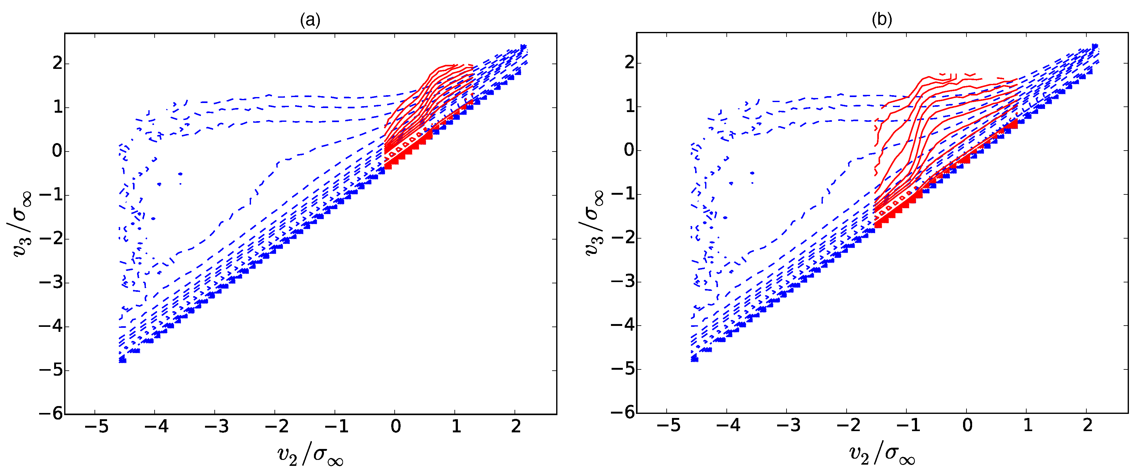
3.3.1. Examination of the Markov Property

The Markov property is fulfilled for the intermediate case as well, provided that the scale separation Δ r is not too small. Figure 21 and Figure 22 show the corresponding contour plots for Δ r = 1.5 λ and Δ r = λ . The shape of the PDFs qualitatively agree with those of the purely nonlocal case; however, for smaller scale separations, one might guess certain differences. The Markov property is not fulfilled for Δ r = 0.2 λ , which can be deduced from Figure 23. The transition PDF (blue) underestimates the v 3 v 2 –correlations of the doubly conditional PDF (red). For comparison, we also refer to Appendix C for an explicit solution for the OK62 transition probability.

3.3.2. Determination of the Markov–Einstein Length

Figure 24 shows the Hellinger distance (36) for five different v 1 . It is remarkable that for v 1 < 0 , the Helligner distance is smaller than for v 1 0 , which only changes for small r. This is also a first hint on the asymmetry of velocity increments in the intermediate case. The latter can be further quantified in considering the evolution in scale of the one -increment PDF in Figure 25a which shows that extreme large negative velocity increments at small scales are more common than positive ones.
Concerning the Hellinger distance itself, we can see that, in contrast to the nonlocal case, the Hellinger distance exhibits a rather pronounced minimum at around Δ r 0.6 λ . This behavior thus resembles somewhat to the behavior encountered in the pure Burgers case and, hence, can be attributed to nonlinear shock generation. Henceforward, the determination of the Markov–Einstein length is rather simple and it can be estimated according to λ M E = 0.6 λ . The latter finding is supported by the semi-logarithmic plot in Figure 24b as well.

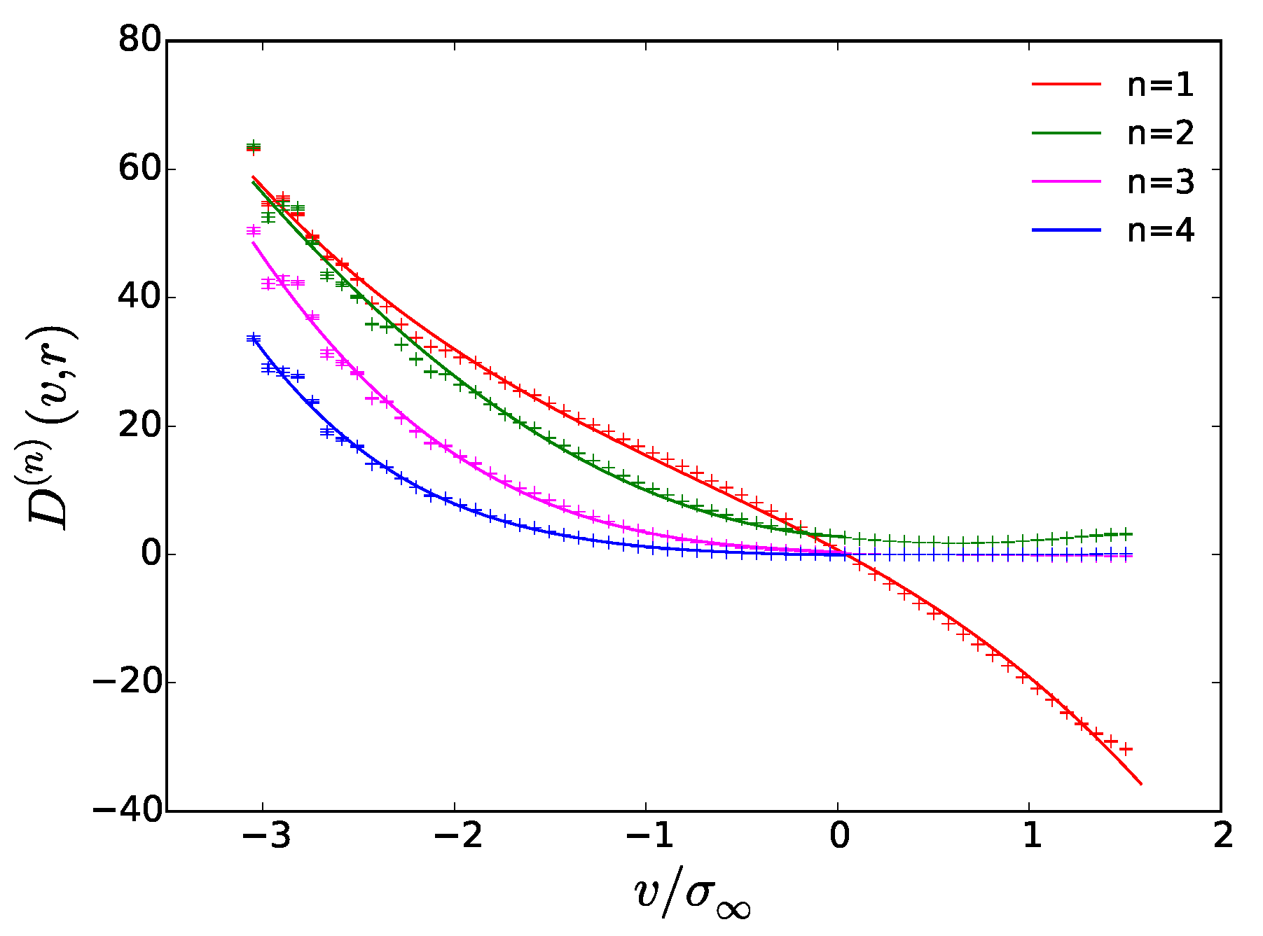
3.3.3. Determination of the Kramers–Moyal Coefficients

The Kramers–Moyal coefficients from run #3 are shown in Figure 25b. The second Kramers–Moyal coefficient exhibits a clear parabolic dependence on v in contrast to the purely nonlocal case, which revealed a linear dependence. The corresponding reduced Kramers–Moyal coefficient K 2 = 0.0208 ± 0.0004 , hence, is roughly ten times bigger than the one determined from the nonlocal case K 2 = 0.0021 ± 0.0001 . The tendency for these intermittency effects also reflects itself in higher-order Kramers–Moyal coefficients n = 3 , 4 . The latter coefficients, even though they appear rather flat, follow a clear v-polynomial of order 3 and 4, respectively.
Moreover, in contrast to the two previous runs #1 and #2, Kramers–Moyal coefficients up to order 9 could significantly be detected and their reduced Kramers–Moyal coefficients could be determined, which will also be discussed in the next section.

4. Quantification of Small-Scale Intermittency on the Basis of Kramers–Moyal Coefficients

We compare the reduced Kramers–Moyal coefficients from runs #1–3 in Figure 26 to the ones predicted by the phenomenological models from Section 2.
For the Burgers case ( α = 1 ), higher-order coefficients ( n = 3 , 4 ) can also be detected significantly for negative increments due to rare large-negative gradient events. Moreover, as discussed in Section 3.1.1, the evolution of the one-increment PDF in scale (Figure 11) showed a pronounced left tail due to shock events. Nonetheless, we could not verify whether this tail corresponds to the predictions of an algebraic tail ( v / r ) 7 / 2 proposed in [15,43]. It has to be stressed that these predictions have been obtained in the context of velocity gradients in Burgers turbulence. The proposed Markov approach, however, solely applies to velocity increments v ( r ) and the limit of velocity gradients r 0 cannot be studied due to the breakdown of the Markov property at small scales (see Section 3.1.1). It is thus not possible to assess the algebraic tail behavior in terms of a solution of the one-increment PDF on the basis of a Kramers–Moyal expansion (7).
Concerning the purely nonlocal case ( α = 0 ), we observed a self-similar evolution of the one-increment PDF in scale which can be seen from Figure 18a. As self-similar behavior is characterized by a single drift coefficient D ( 1 ) , higher order Kramers–Moyal coefficients should be close to zero. In fact, Figure 18b shows that D ( 3 ) and D ( 4 ) are rather small. Furthermore, the diffusion coefficient D ( 2 ) is linear in v and has only a small reduced Kramers–Moyal coefficient K 2 = 0.0021 ± 0.0001 . Finally, K 1 = 0.3108 ± 0.0002 suggests that the purely nonlocal case can be described quite accurately by the K41 theory i.), which has already been reported in [24].
Higher order K n of the intermediate case ( α = 0.15 ) correspond well to Yakhot’s intermittency model. However, it must be stressed that the first three coefficients deviate from Yakhot’s predictions (red curve in Figure 26). Moreover, in calculating the third-order structure function ζ 3 = 3 K 1 3 K 2 + K 3 1.266 , we observe that it does not follow Kolmogorov’s law. Hence, an accurate description via the Kramers–Moyal coefficients has to resolve the spatial dependence of D ( n ) ( v , r ) as well in order to extract the 1 / r dependence. Nevertheless, one can clearly distinguish between the green (She–Leveque model) and red curve (Yakhot’s model), which is usually not possibly on the basis of a mere scaling exponent analysis.

5. Conclusions and Outlook

The present paper underlines the importance of the multi-scale approach devised by Friedrich and Peinke [8], which is capable of capturing the general effects of anomalous scaling in turbulence embodied in Equation (17). An admissible description of intermittency in turbulence, however, should take into account an infinite number of Kramers–Moyal coefficients, which has been demonstrated by the semi-logarithmic plots of the reduced Kramers–Moyal coefficients in Figure 2b and Figure 26. Further work will be dedicated to the investigation of higher-order Kramers–Moyal coefficients in the experiment and in DNS of 3D turbulence in [44]. In this context, the presented semi-logarithmic plot in Figure 26 might as well be a more accurate method for the determination of possible scaling behavior than the usual structure function plot Figure 1. This would open the possibility to decide which of the various phenomenological models is best suited to describe 3D Navier–Stokes turbulence. In the case of artificial generalized Burgers turbulence, the Yakhot’s mean field model [29] could clearly be confirmed as the most accurate candidate. In order to further assess the role of advection by the nonlinearity and nonlocality introduced by the pressure term, the study of other model systems than Equation (26), e.g., the modified three-dimensional Navier–Stokes equation proposed by Grafke, Grauer and Sideris [45] seems to be highly relevant.
Moreover, the Kramers–Moyal approach should yield important insights on the ongoing discussion about different intermittency behavior between longitudinal and transverse structure functions. Here, the simple rescaling relation between longitudinal and transverse structure functions [46,47] might be extended to allow for different intermittency in tuning the corresponding set of reduced Kramers–Moyal coefficients in Equation (17).

Author Contributions

Conceptualization, J.F., R.G.; methodology, J.F., R.G.; validation, J.F., R.G., writing—original draft preparation, J.F., R.G.; writing—review and editing, J.F., R.G. All authors have read and agreed to the published version of the manuscript.

Funding

J.F. acknowledges funding from the Humboldt Foundation within a Feodor–Lynen fellowship and benefited from financial support through the Project IDEXLYON of the University of Lyon in the framework of the French program “Programme Investissements d’Avenir” (ANR-16-IDEX-0005). Parts of this research were supported by the DFG-Research Unit FOR 1048, project B2.

Acknowledgments

J.F. is grateful for discussions with Joachim Peinke, Alain Pumir, and Oliver Kamps.

Conflicts of Interest

The authors declare no conflict of interest.

Appendix A. Solutions for the Transition Probabilities of Burgers Turbulence

In the following, we want to discuss solutions of the transition PDF for certain phenomenological models of turbulence. The point of departure is the Kramers–Moyal expansion for the transition PDF (8). We first discuss the solutions of the Kramers–Moyal coefficients of the Burgers phenomenology for ramp and shock solutions (22).

Appendix A.1. Shock Solution

The Burgers Kramers–Moyal expansion for the transition PDF of the shocks reads
r p ( v , r | v , r ) = n = 1 1 n ! n v n v n r p ( v , r | v , r ) ,
A solution of this equation can be obtained from its Dyson series representation
p ( v , r | v , r ) = δ ( v v ) + r r d r 1 L ^ K M ( v , r 1 ) δ ( v v ) + r r d r 1 r r 1 d r 2 L ^ K M ( v , r 1 ) L ^ K M ( v , r 2 ) δ ( v v ) + = δ ( v v ) + r r d r 1 L ^ r 1 δ ( v v ) + r r d r 1 r r 1 d r 2 L ^ 2 r 1 r 2 δ ( v v ) + = δ ( v v ) + ln r r L ^ δ ( v v ) + 1 2 ! ln r r 2 L ^ 2 δ ( v v ) + = exp ln r r L ^ δ ( v v ) ,
where the differential operator L ^ is defined according to
L ^ = n = 1 K n n ! n v n v n .
For Burgers-shocks, we have K n = 1 for all n and thus the operator reads
L ^ = n = 1 1 n ! n v n v n .
We can now let this operator act on the delta function and obtain
L ^ δ ( v v ) = n = 1 1 n ! n v n v n δ ( v v ) ,
where we put the sifting property of the delta function into use. Now, we can write the delta function in its Fourier representation and obtain
L ^ δ ( v v ) = n = 1 1 n ! n v n v n d u 2 π e i u ( v v ) = n = 1 d u 2 π ( i u v ) n n ! e i u ( v v ) = d u 2 π e i u ( v v ) d u 2 π e i u v e i u ( v v ) = δ ( v v ) δ ( v ) ,
Another application of the operator yields
L ^ 2 δ ( v v ) = L ^ δ ( v v ) L ^ δ ( v ) = δ ( v v ) + δ ( v ) ,
Inserting this result into Equation (A2) yields
p ( v , r | v , r ) = δ ( v v ) ln r r ( δ ( v v ) δ ( v ) ) + 1 2 ! ln r r 2 ( δ ( v ) δ ( v v ) ) + = e ln r r δ ( v v ) + ( 1 e ln r r ) δ ( v ) .
The transition PDF for negative increments v of the Burgers phenomenology thus reads
p ( v , r | v , r ) = r r δ ( v v ) + 1 r r δ ( v ) .
It can be verified that this solution yields the correct Kramers–Moyal coefficients
D ( n ) ( v , r ) = 1 n ! lim r r 1 r r d v ( v v ) n p ( v , r | v , r ) = 1 n ! d v ( v v ) n p ( v , r | v , r ) r | r = r = 1 n ! d v ( v v ) n 1 r δ ( v v ) 1 r δ ( v ) = ( 1 ) n n ! v n r .
At the same time, it is also provable that the transition PDF (A9) satisfies the coincidence property
lim r r p ( v , r | v , r ) = δ ( v v ) .

Appendix A.2. Ramp Solution

The Fokker–Planck equation for the transition PDF of positive velocity increments in Burgers turbulence reads
r p ( v , r | v , r ) = v v r p ( v , r | v , r ) ,
which is a first-order partial differential equation. Therefore, we can obtain a solution through the method of characteristics (see next section). The same solution can also be acquired from the Dyson series (A2) and involves interesting commutation relations of the Fokker–Planck operator in Equation (A12).

Appendix A.2.1. Solution by the Method of Characteristics

The method of characteristics [48] suggests that we write the transition PDF in Equation (A12) in dependence of the parameter λ as p ( v ( λ ) , r ( λ ) | v , r ) , which can be derived with respect to λ according to
d d λ p ( v ( λ ) , r ( λ ) | v , r ) = p ( v ( λ ) , r ( λ ) | v , r ) r ( λ ) r ˙ ( λ ) + p ( v ( λ ) , r ( λ ) | v , r ) v ( λ ) v ˙ ( λ ) .
Comparing this to Equation (A12), we obtain the following ordinary differential equations
r ˙ ( λ ) = 1 v ˙ ( λ ) = v ( λ ) r ( λ ) d p ( v ( λ ) , r ( λ ) | v , r ) d λ = p ( v ( λ ) , r ( λ ) | v , r ) r ( λ ) .
Integrating the second and the third equation from r to r with the initial condition δ ( v v ) for p yields
v ( λ ) = v r ( λ ) r p ( v ( λ ) , r ( λ ) | v , r ) = δ ( v v ) r r ( λ ) ,
Therefore, the transition for positive velocity increments v of the Burgers phenomenology reads
p ( v , r | v , r ) = δ v r r v .
Again, the transition PDF yields the correct Kramers–Moyal coefficients (10) and satisfies the coincidence property.

Appendix A.2.2. Solution from Dyson Series

The Dyson series (A2) for Equation (A12) reads
p ( v , r | v , r ) = δ ( v v ) ln r r v v δ ( v v ) + 1 2 ! ln r r 2 v v 2 δ ( v v ) +
We thus have to evaluate the following operator products
v v v v v v n - times δ ( v v ) .
Using the sifting property of the delta function, we rewrite Equation (A18) according to
v v v v v v n - times = v n v n ( n 1 ) n 1 v n 1 v n 1 + = k = 0 n 1 n 1 k n k v n k v n k ( 1 ) k .
Writing the delta function in its Fourier-representation, we acquire
p ( v , r | v , r ) = d u 2 π 1 + n = 0 k = 0 n 1 ln r r n n ! n k v n k v n k ( 1 ) k e i u ( v v ) = d u 2 π 1 + n = 0 k = 0 n 1 ln r r n n ! ( i u v ) n k e i u ( v v ) = d u 2 π n = 0 ( i u v ) n n ! exp ln r r 1 n e i u ( v v ) = d u 2 π exp i u v ( r r 1 ) e i u ( v v ) = δ v r r v ,
which is the same solution that we gained from the method of characteristics (A16).

Appendix B. Solution for the Transition Probability of the K41 Phenomenology

The Fokker–Planck equation for the transition PDF of the K41 phenomenology discussed in Section (Section 2) under (i.) reads
r p ( v , r | v , r ) = v v 3 r p ( v , r | v , r ) .
Again, this equation can be solved with the method of characteristics [48] and we reach the system of equations
r ˙ ( λ ) = 1 v ˙ ( λ ) = v ( λ ) 3 r ( λ ) d p ( v ( λ ) , r ( λ ) | v , r ) d λ = p ( v ( λ ) , r ( λ ) | v , r ) 3 r ( λ ) ,
which has the solution
p ( v , r | v , r ) = δ v r 1 / 3 r 1 / 3 v .

Appendix C. Solution for the Transition Probability of the OK62 Phenomenology

The OK62 phenomenology was already discussed in Section 2 under (ii.) and is equivalent to a Fokker–Planck equation
r p ( v , r | v , r ) = v 3 + μ 9 r v 2 v 2 μ 18 r v 2 p ( v , r | v , r ) .
We introduce
A = 3 + μ 9 B = μ 18 ,
and choose our ansatz as a log-normal distribution of the form
p ( v , r | v , r ) = 1 2 π Q ( r , r ) v exp ln v v K ( r , r ) 2 2 Q ( r , r ) ,
where K ( r , r ) and Q ( r , r ) are functions that are yet to be determined by Equation (A24). Deriving Equation (A26) with respect to r yields
r p ( v , r | v , r ) = Q ˙ 2 Q + ln v v K Q K ˙ + ln v v K 2 2 Q 2 Q ˙ p ( v , r | v , r ) ,
where the dot indicates a derivative with respect to r.
The right-hand side of Equation (A24) is evaluated as follows:
v v p ( v , r | v , r ) = ln v v K Q p ( v , r | v , r ) ,
and
2 v 2 v 2 p ( v , r | v , r ) = 1 Q ln v v K Q + ln v v K 2 Q 2 p ( v , r | v , r ) .
The determining equation for K ( r , r ) and Q ( r , r ) thus reads
Q ˙ 2 Q + ln v v K Q K ˙ + ln v v K 2 2 Q 2 Q ˙ = B Q r + A r B r ln v v K Q + B r ln v v K 2 Q 2 ,
and we can read off the following ordinary differential equations for K ( r , r ) and Q ( r , r )
Q ˙ ( r , r ) = 2 B r ,
K ˙ ( r , r ) = A r B r ,
which can be integrated according to
Q ( r , r ) = 2 b ln r r ,
K ( r , r ) = a ln r r ,
where
a = A B = 1 3 + μ 6 b = B = μ 18 .
The exact solution for the transition probability of this particular Fokker–Planck equation of the OK62 phenomenology then reads
p ( v , r | v , r ) = 1 4 π b ln r r v exp ln v v a ln r r 2 4 b ln r r .
We find that for r r , the transition probability approaches a delta function, according to
lim r r p ( v , r | v , r ) = 1 v δ ln v v = δ ( v v ) ,
which is in accordance with the coincidence property.
In the following, we investigate the relation of the transition PDF (A36) to the one-increment PDF proposed by Yakhot [30] as well as by Castaing [49]. In using the so-called Mellin transform, Yakhot was able to derive the one-increment PDF directly from the structure functions of the OK62 phenomenology. Furthermore, he assumed that the PDF follows a Gaussian distribution at large scales, e.g., for r = 1 he stated that f 1 ( v , r = 1 ) = e v 2 / 2 2 π . Yakhot’s formula can be obtained from the transition PDF (A36) in setting r = 1 and making use of the reduction property of the two-increment PDF
f 1 ( v , r ) = d v p ( v , r | v , r = 1 ) f 1 ( v , r = 1 ) = 1 π v 8 b ln r d v e v 2 / 2 exp ln v a ln r ln v 2 4 b ln r ,
which reduces to a Gaussian for r = 1 , as demanded.
In analogy with the OK62 phenomenology, Castaing’s model of a multiplicative energy cascade is based on local fluctuations of the energy dissipation rate, which follow a log-normal distribution. However, in contrast to OK62, which predicts scaling of the structure functions, Castaing’s formula
f 1 ( v , r ) = 1 2 π λ ( r ) d s s 2 exp ln 2 ( s / s 0 ( r ) ) 2 λ 2 ( r ) e v 2 / 2 s 2 ,
was devised to fit experimental data via the fitting functions s 0 ( r ) and λ ( r ) and does not necessarily imply structure function scaling. Castaing’s formula (A39) is more general than Yakhot’s formula (A38), which can be recovered in substituting s = v / v and choosing s 0 ( r ) = r a and λ ( r ) = 2 b ln r .

References

  1. Nelkin, M. In what sense is turbulence an unsolved problem? Science 1992, 255, 566–570. [Google Scholar] [CrossRef] [PubMed]
  2. Monin, A.S.; Yaglom, A.M. Statistical Fluid Mechanics: Mechanics of Turbulence; Courier Dover Publications: Mineola, NY, USA, 2007. [Google Scholar]
  3. Kolmogorov, A.N. The local structure of turbulence in incompressible viscous fluid for very large Reynolds numbers. C. R. Acad. Sci. URSS 1941, 30, 301–305. [Google Scholar]
  4. Kolmogorov, A.N. A refinement of previous hypotheses concerning the local structure of turbulence in a viscous incompressible fluid at high Reynolds number. J. Fluid Mech. 1962, 13, 82–85. [Google Scholar] [CrossRef] [Green Version]
  5. Oboukhov, A.M. Some specific features of atmospheric tubulence. J. Fluid Mech. 1962, 13, 77. [Google Scholar] [CrossRef]
  6. She, Z.S.; Leveque, E. Universal scaling laws in fully developed turbulence. Phys. Rev. Lett. 1994, 72, 336–339. [Google Scholar] [CrossRef] [PubMed]
  7. Frisch, U. Turbulence; Cambridge University Press: Cambridge, UK, 1995. [Google Scholar]
  8. Friedrich, R.; Peinke, J. Description of a Turbulent Cascade by a Fokker–Planck Equation. Phys. Rev. Lett. 1997, 78, 863–866. [Google Scholar] [CrossRef]
  9. Lück, S.; Renner, C.; Peinke, J.; Friedrich, R. The Markov–Einstein coherence length-a new meaning for the Taylor length in turbulence. Phys. Lett. A 2006, 359, 335–338. [Google Scholar] [CrossRef]
  10. Renner, C. Markowanalysen Stochastisch Fluktuierender Zeitserien. Ph.D. Thesis, Carl von Ossietzky Universität Oldenburg, Oldenburg, Germany, 2002. [Google Scholar]
  11. Friedrich, R.; Peinke, J.; Sahimi, M.; Tabar, R.M. Approaching complexity by stochastic methods: From biological systems to turbulence. Phys. Rep. 2011, 506, 87–162. [Google Scholar] [CrossRef]
  12. Hopf, E. The partial differential equation ut + uux = μxx. Commun. Pure Appl. Math. 1950, 3, 201–230. [Google Scholar] [CrossRef]
  13. Cole, J.D. On a quasi-linear parabolic equation occuring in aerodynamics. Q. Appl. Math. 1951, 9, 225–236. [Google Scholar] [CrossRef] [Green Version]
  14. Polyakov, A.M. Turbulence without pressure. Phys. Rev. E 1995, 52, 6183–6188. [Google Scholar] [CrossRef] [PubMed] [Green Version]
  15. E, W.; Vanden Eijnden, E. Asymptotic Theory for the Probability Density Functions in Burgers Turbulence. Phys. Rev. Lett. 1999, 83, 2572–2575. [Google Scholar] [CrossRef] [Green Version]
  16. Bouchaud, J.P.; Mézard, M. Velocity fluctuations in forced Burgers turbulence. Phys. Rev. E 1996, 54, 5116. [Google Scholar] [CrossRef] [PubMed] [Green Version]
  17. Eule, S.; Friedrich, R. A note on the forced Burgers equation. Phys. Lett. A 2006, 351, 238–241. [Google Scholar] [CrossRef] [Green Version]
  18. Friedrich, J.; Margazoglou, G.; Biferale, L.; Grauer, R. Multiscale velocity correlations in turbulence and Burgers turbulence: Fusion rules, Markov processes in scale, and multifractal predictions. Phys. Rev. E 2018, 98, 023104. [Google Scholar] [CrossRef] [Green Version]
  19. Bec, J.; Khanin, K. Burgers turbulence. Phys. Rep. 2007, 447, 1–66. [Google Scholar] [CrossRef]
  20. Zel’Dovich, Y.B. Gravitational instability: An approximate theory for large density perturbations. Astron. Astrophys. 1970, 5, 84–89. [Google Scholar]
  21. Hussain, S.; Mahmood, S. Korteweg-de Vries Burgers equation for magnetosonic wave in plasma. Phys. Plasmas 2011, 18, 052308. [Google Scholar] [CrossRef]
  22. Dreher, J.; Ruban, V.; Grauer, R. Axisymmetric flows in Hall-MHD: A tendency towards finite-time singularity formation. Phys. Scr. 2005, 72, 451. [Google Scholar] [CrossRef] [Green Version]
  23. Kardar, M.; Parisi, G.; Zhang, Y.C. Dynamic scaling of growing interfaces. Phys. Rev. Lett. 1986, 56, 889. [Google Scholar] [CrossRef] [Green Version]
  24. Zikanov, O.; Thess, A.; Grauer, R. Statistics of turbulence in a generalized random-force-driven Burgers equation. Phys. Fluids 1997, 9, 1362. [Google Scholar] [CrossRef]
  25. Risken, H. The Fokker–Planck Equation; Springer: Berlin/Heidelberg, Germany, 1996. [Google Scholar]
  26. Tang, S.; Antonia, R.; Djenidi, L.; Zhou, Y. Scaling of the turbulent energy dissipation correlation function. J. Fluid Mech. 2020, 891, A26. [Google Scholar] [CrossRef]
  27. Nickelsen, D. Markov Processes linking Thermodynamics and Turbulence. arXiv 2015, arXiv:1510.06281. [Google Scholar]
  28. Nickelsen, D. Master equation for She–Leveque scaling and its classification in terms of other Markov models of developed turbulence. J. Stat. Mech. Theory Exp. 2017, 2017, 073209. [Google Scholar] [CrossRef] [Green Version]
  29. Yakhot, V. Mean-field approximation and a small parameter in turbulence theory. Phys. Rev. E 2001, 63, 26307. [Google Scholar] [CrossRef] [Green Version]
  30. Yakhot, V. Probability densities in strong turbulence. Physics D 2006, 215, 166–174. [Google Scholar] [CrossRef] [Green Version]
  31. Novikov, E.A. Infinitely divisible distributions in turbulence. Phys. Rev. E 1994, 50, R3303–R3305. [Google Scholar] [CrossRef]
  32. Castaing, B. The Temperature of Turbulent Flows. J. Phys. II 1996, 6, 105–114. [Google Scholar] [CrossRef]
  33. Eling, C.; Oz, Y. The anomalous scaling exponents of turbulence in general dimension from random geometry. J. High Energy Phys. 2015, 2015, 150. [Google Scholar] [CrossRef] [Green Version]
  34. Pawula, R.F. Approximation of the Linear Boltzmann Equation by the Fokker–Planck Equation. Phys. Rev. 1967, 162, 186–188. [Google Scholar] [CrossRef]
  35. Renner, C.; Peinke, J.; Friedrich, R. Experimental indications for Markov properties of small-scale turbulence. J. Fluid Mech. 2001, 433, 383–409. [Google Scholar] [CrossRef]
  36. Chekhlov, A.; Yakhot, V. Kolmogorov turbulence in a random-force-driven Burgers equation. Phys. Rev. E 1995, 51, 4–7. [Google Scholar] [CrossRef] [PubMed] [Green Version]
  37. Sagaut, P.; Cambon, C. Governing Equations, from Dynamics to Statistics. In Homogeneous Turbulence Dynamics; Springer International Publishing: Berlin/Heidelberg, Germany, 2018; pp. 13–73. [Google Scholar]
  38. Shu, C.W.; Osher, S. Efficient implementation of essentially non-oscillatory shock-capturing schemes. J. Comput. Phys. 1988, 77, 439–471. [Google Scholar] [CrossRef] [Green Version]
  39. Hou, T.Y.; Li, R. Computing nearly singular solutions using pseudo-spectral methods. J. Comput. Phys. 2007, 226, 379–397. [Google Scholar] [CrossRef] [Green Version]
  40. Higham, D. An Algorithmic Introduction to Numerical Simulation of Stochastic Differential Equations. SIAM Rev. 2001, 43, 525–546. [Google Scholar] [CrossRef]
  41. Balkovsky, E.; Falkovich, G.; Kolokolov, I.; Lebedev, V. Intermittency of Burgers’ Turbulence. Phys. Rev. Lett. 1997, 78, 1452–1455. [Google Scholar] [CrossRef] [Green Version]
  42. Hellinger, E. Neue Begründung der Theorie quadratischer Formen von unendlichvielen Veränderlichen. J. Reine Angew. Math. 1909, 1909, 210–271. [Google Scholar] [CrossRef]
  43. Bec, J. Universality of Velocity Gradients in Forced Burgers Turbulence. Phys. Rev. Lett. 2001, 87, 104501. [Google Scholar] [CrossRef] [Green Version]
  44. Friedrich, J. Closure of the Lundgren-Monin-Novikov Hierarchy in Turbulence Via a Markov Property of Velocity Increments in Scale. Ph.D. Thesis, Ruhr-University Bochum, Bochum, Germany, 2017. [Google Scholar]
  45. Grafke, T.; Grauer, R.; Sideris, T.C. Turbulence properties and global regularity of a modified Navier–Stokes equation. Phys. D Nonlinear Phenom. 2013, 254, 18–23. [Google Scholar] [CrossRef] [Green Version]
  46. Grauer, R.; Homann, H.; Pinton, J.F. Longitudinal and transverse structure functions in high-Reynolds-number turbulence. New J. Phys. 2012, 14, 63016. [Google Scholar] [CrossRef] [Green Version]
  47. Friedrich, J.; Homann, H.; Schäfer, T.; Grauer, R. Longitudinal and transverse structure functions in high Reynolds-number magneto-hydrodynamic turbulence. New J. Phys. 2016, 18, 125008. [Google Scholar] [CrossRef]
  48. Courant, R.; Hilbert, D. Methods of Mathematical Physics II; Wiley: Hoboken, NJ, USA, 1962. [Google Scholar]
  49. Castaing, B.; Gagne, Y.; Hopfinger, E.J. Velocity probability density functions of high Reynolds number turbulence. Phys. D Nonlinear Phenom. 1990, 46, 177–200. [Google Scholar] [CrossRef]
Figure 1. Scaling exponents ζ n of velocity structure functions for the different phenomenologies discussed in (i.)–(vi.). The crosses that are arranged on the straight n / 3 -line correspond to the self-similar K41 phenomenology (i.). Burgers phenomenology (iii.) exhibits the strongest intermittency behavior whereas the other phenomenologies can only be distinguished for higher orders n. Note that the OK62 phenomenology (ii.) has a parabolic form that violates the structure function convexity condition [7] for n 3 2 + 3 μ (not observable in the figure).
Atmosphere 11 01003 g001
Figure 2. (a) reduced Kramers–Moyal coefficients from Equation (17) for different phenomenological models of turbulence up to the order n = 10 . Coefficients for n > 2 seem to tend towards zero; (b) semi-logarithmic plot of the reduced Kramers–Moyal coefficients. All phenomenological models except for K41 and OK62 show an asymptotic behavior. Note that the She–Leveque model possesses a nearly linear slope in the semi-logarithmic representation.
Atmosphere 11 01003 g002
Figure 3. (a) typical realization of the velocity field u ( x , t ) in DNS of Burgers turbulence ( α = 1 in Equation (26)). The velocity field exhibits a sawtooth profile that is due to the formation of large negative velocity gradients; (b) velocity field realization that belongs to the largest velocity gradient attained in the DNS belonging to Table 1.
Atmosphere 11 01003 g003
Figure 4. (a) energy spectrum E ( k , t ) of the velocity field of DNS of Burgers turbulence. The small wavenumbers (largest scales) show nearly Kolmogorov-like behavior k 5 / 3 whereas a shock-like behavior k 2 can be perceived for a small band of larger wavenumbers at the edge of the inertial range. The dissipation range exhibits an exponential decay of the energy spectrum. Inertial range limits have been indicated by k L and k η and are explained in detail in the plain text; (b) compensated energy spectra E ( k ) / k a . The blue lines correspond to the Kolmogorov case a = 5 / 3 and the green line to the shock case a = 2 . Constant lines in the plot indicate scaling behavior of the spectrum. The spectrum for smaller wavenumbers is quite close to the Kolmogorov spectrum. Larger wavenumbers in the inertial range at around 60 < k < 80 show more of a shock-like spectrum; in addition, the compensated spectrum is not as flat as in the Kolmogorov case.
Atmosphere 11 01003 g004
Figure 5. Evolution of the velocity increment PDF in scale (multiples of the Taylor length λ ) for the Burgers case α = 1 . The PDFs are shifted vertically and normed with their corresponding standard deviation σ r for improved visualization. The pronounced left part of the PDFs is dominated by small-scale shock events, whereas the right part exhibits nearly self-similar behavior.
Atmosphere 11 01003 g005
Figure 6. (a) examination of the Markov property (28) from DNS of Burgers turbulence for r = 2 λ and v 1 = 0 via a logarithmic contour plot. The dashed blue contour lines correspond to p ( v 3 , L / 2 Δ r | v 2 , L / 2 ) whereas the red lines correspond to p ( v 3 , L / 2 Δ r | v 2 , L / 2 ; v 1 , L / 2 + Δ r ) . The Markov property is fulfilled only approximately. Although the contours exhibit an almost identical shape, they seem to be slightly displaced. The shape of the transition PDF (blue) can be reproduced for the most part by the theoretical predictions (31); (b) same as in (a), but for v 1 = σ . A broader part of the blue dashed lines that belong to p ( v 3 , L / 2 Δ r | v 2 , L / 2 ) can be covered in comparison to (a). Event though the red contour lines indicate insufficient statistics in the boundary regions, the Markov property has not deteriorated in comparison to (a).
Atmosphere 11 01003 g006
Figure 7. (a) examination of the Markov property (28) from DNS of Burgers turbulence for Δ r = λ and v 1 = 0 . The Markov property seems to hold quite well for this set of parameters; (b) same as in (a), but for v 1 = σ . A broader part of the blue dashed lines that belong to p ( v 3 , L / 2 Δ r | v 2 , L / 2 ) The Markov property has not deteriorated in comparison to (a).
Atmosphere 11 01003 g007
Figure 8. (a) examination of the Markov property (28) from DNS of Burgers turbulence for Δ r = 0.2 λ and v 1 = 0 . The Markov property is violated as the transition PDF (red) overestimates the correlations that is exhibited by the conditional PDF (blue); (b) same as in (a), but for v 1 = σ . The violation of the Markov property becomes even more pronounced.
Atmosphere 11 01003 g008
Figure 9. (a) Hellinger distance d H ( Δ r ) for different v 1 and variable step width Δ r . Apparently, the Markov property only is a good approximation around Δ r = λ . For larger Δ r , the Hellinger distance slightly increases and approaches a small constant value. However, for smaller Δ r , the Hellinger distance exhibits a clearer increase. These tendencies become even more pronounced for v 1 = 0.33 σ , 0.66 σ , σ ; (b) semi-logarithmic plot of the Hellinger distance d H ( Δ r ) . For Δ r < 0.8 λ , the Hellinger distance seems to increase nearly exponentially.
Atmosphere 11 01003 g009
Figure 10. Conditional moments of first order divided by scale separation Δ r , M ( 1 ) ( v , r ; Δ r ) / Δ r for r = L / 2 , (a) v 1 = 2.5 σ , (b) v 1 = 0.46875 σ , (c) v 1 = 1.25 σ and variable Δ r . The fits correspond to polynomials of second order in Δ r for Δ r > λ M E . Note that the Δ r -axis has been rescaled by the Markov–Einstein-length λ M E and the conditional moment drops to zero for Δ r < λ M E .
Atmosphere 11 01003 g010
Figure 11. Estimation of the Kramers–Moyal coefficients from DNS of Burgers turbulence for r = L / 2 . The fits correspond to polynomials of the order n of the coefficient except for n = 1 where a polynomial of order three has been used. The reduced Kramers–Moyal coefficients have been determined according to K 1 = 1.1689 ± 0.08 , K 2 = 0.7880 ± 0.14 , K 3 = 0.6956 ± 0.17 and K 4 = 0.7137 ± 0.12 .
Atmosphere 11 01003 g011
Figure 12. (a) typical realization of the velocity field u ( x , t ) in DNS of the purely nonlocal case ( α = 0 in Equation (26)). The velocity field is not composed of shocks as in Burgers turbulence, but rather shows cusp-like structures; (b) velocity field realization that belongs to the largest velocity field gradient that was attained in the DNS belonging to run #2 in Table 1.
Atmosphere 11 01003 g012
Figure 13. (a) energy spectrum E ( k , t ) of the velocity field of DNS of the nonlocal case. The inertial range obeys a Kolmogorov-like behavior k 5 / 3 . (b) compensated energy spectrum E ( k ) / k 5 / 3 .
Atmosphere 11 01003 g013
Figure 14. (a) examination of the Markov property (28) from DNS of the nonlocal case for Δ r = 2.2 λ and v 1 = 0 via a logarithmic contour plot. (b) same as in (a), but for v 1 = σ . The shape of the conditional PDF (red) does not change significantly in comparison to (a).
Atmosphere 11 01003 g014
Figure 15. (a) examination of the Markov property (28) from DNS of the nonlocal case for Δ r = 1 λ and v 1 = 0 via a logarithmic contour plot. (b) same as in (a), but for v 1 = σ .
Atmosphere 11 01003 g015
Figure 16. (a) examination of the Markov property (28) from DNS of the nonlocal case for Δ r = 0.2 λ and v 1 = 0 via a logarithmic contour plot. (b) same as in (a), but for v 1 = σ . The Markov property is violated.
Atmosphere 11 01003 g016
Figure 17. (a) Hellinger distance d H ( Δ r ) for different v 1 and variable step width Δ r for the purely nonlocal case. The Hellinger is close to zero and only increases at around Δ r λ ; (b) semi-logarithmic plot of the Hellinger distance d H ( Δ r ) .
Atmosphere 11 01003 g017
Figure 18. (a) evolution of the velocity increment PDF in scale for the purely nonlocal case α = 0 . The PDFs exhibit self-similarity in the inertial range; (b) estimation of the Kramers–Moyal coefficients D ( n ) ( v , r = L / 2 ) from DNS of the purely nonlocal case α = 0 . The fits correspond to polynomials of the order n of the coefficient except for n = 1 where a polynomial of order three has been used. The reduced Kramers–Moyal coefficients have been determined according to K 1 = 0.3108 ± 0.0002 , K 2 = 0.0021 ± 0.0001 , K 3 = ( 2.64 ± 0.01 ) × 10 5 and K 4 = ( 2.28 ± 2.56 ) × 10 5 .
Atmosphere 11 01003 g018
Figure 19. (a) typical realization of the velocity field u ( x , t ) in DNS of the intermediate case ( α = 0.15 in Equation (26)); (b) velocity field realization that belongs to the largest velocity field gradient that was attained in the DNS.
Atmosphere 11 01003 g019
Figure 20. Energy spectrum E ( k ) from DNS of the intermediate regime ( α = 0.15 ). The line indicates the spectral slope k 1.18 . No clear power–law behavior of the energy spectrum could be detected. The Kolmogorov spectrum might as well appear for larger k behind the indicated spectral slope.
Atmosphere 11 01003 g020
Figure 21. (a) examination of the Markov property (28) from DNS of the intermediate case for Δ r = 2.2 λ and v 1 = 0 via a logarithmic contour plot. (b) same as in (a), but for v 1 = σ . The shape of the conditional PDF (red) does not change significantly in comparison to (a).
Atmosphere 11 01003 g021
Figure 22. (a) examination of the Markov property (28) from DNS of the intermediate case for r = 1 λ and v 1 = 0 via a logarithmic contour plot; (b) same as in (a), but for v 1 = σ .
Atmosphere 11 01003 g022
Figure 23. (a) examination of the Markov property (28) from DNS of the intermediate case for Δ r = 0.2 λ and v 1 = 0 via a logarithmic contour plot; (b) same as in (a), but for v 1 = σ . The Markov property is violated.
Atmosphere 11 01003 g023
Figure 24. (a) Hellinger distance d H ( Δ r ) for different v 1 and variable step width Δ r . Apparently, the Markov property is a good approximation only around Δ r = λ . For larger Δ r , the Hellinger distance slightly increases and approaches a small constant value. However, for smaller Δ r , the Hellinger distance exhibits a more pronounced increase. Therefore, the Markov property is clearly violated. These effects become even more pronounced for v 1 = 0.33 σ , 0.66 σ , , σ . (b) Semi-logarithmic plot of the Hellinger distance d H ( Δ r ) . For r < 0.8 λ , the Hellinger distance seems to increase nearly exponentially.
Atmosphere 11 01003 g024
Figure 25. (a) evolution of the velocity increment PDF in scale for the intermediate case α = 0.15 . The PDFs show a slight asymmetry at small scales. (b) estimation of the Kramers–Moyal coefficients from DNS of the intermediate case α = 0.15 . The fits correspond to polynomials of the order n of the coefficient except for n = 1 where a polynomial of order three has been used. The reduced Kramers–Moyal coefficients have been determined according to K 1 = 0.4356 ± 0.0007 , K 2 = 0.0208 ± 0.0004 , K 3 = 0.0014 ± 0.0001 and K 4 = 0.00041 ± 0.00001 .
Atmosphere 11 01003 g025
Figure 26. Semi-logarithmic plot of reduced Kramers–Moyal coefficients from DNS of the generalized Burgers Equation (26). The coefficients for Burgers turbulence ( α = 1 ) are in the range of 1 which agrees with the phenomenological predictions. The semi-logarithmic plot reveals that the reduced Kramers–Moyal coefficients for the intermediate case ( α = 0.15 ) follow Yakhot’s mean field theory (v.). Note that higher-order n > 5 coefficients for the Burgers and the purely nonlocal case ( α = 0 ) could not be accurately obtained due to poor polynomial fits (Burgers case) or considerable deviations from Equation (17) (nonlocal case).
Atmosphere 11 01003 g026
Table 1. Characteristic parameters of the numerical simulations: root mean square velocity u r m s = u 2 , viscosity ν , averaged rate of local energy dissipation ε = 2 ν u x 2 , grid spacing dx, dissipation length η = ν 3 ε 1 / 4 , Taylor length λ = u r m s ν ε , Taylor-Reynolds number Re λ = u r m s λ ν , integral length scale L = u r m s 3 ε , large-eddy turn-over time T L = L u r m s , number of grid points N and cut-off of the power law forcing. The intermediate case ( α = 0.15 ) included a damping term of the form γ u ( x , t ) with γ = 0.002 on the r.h.s. of Equation (26).
run#1 ( α = 1 )#2 ( α = 0 )#3 ( α = 0.15 )
u r m s 0.00790.00580.0026
ν 0.0000140.00001 1 × 10 6
ε 5.45 × 10 7 1.38 × 10 7 6.23 × 10 8
dx0.0020.00150.0015
η 0.00840.00920.002
λ 0.04010.048950.0104
Re λ 22.7128.166827.36
L0.91191.3790.286
T in T L 744110572299
n307240964096
cut-off305240664066

