Article

An Updated Synoptic Climatology of Lake Erie and Lake Ontario Heavy Lake-Effect Snow Events

Department of Geosciences, Mississippi State University, 75 B. S. Hood Road, Mississippi State, MS 39762, USA
*
Author to whom correspondence should be addressed.
Atmosphere 2020, 11(8), 872; https://doi.org/10.3390/atmos11080872
Submission received: 3 June 2020 / Revised: 3 August 2020 / Accepted: 11 August 2020 / Published: 17 August 2020
(This article belongs to the Section Meteorology)

Abstract

:
Lake-effect snow (LES) storms pose numerous hazards, including extreme snowfall and blizzard conditions, and insight into the large-scale precursor conditions associated with LES can aid local forecasters and potentially allow risks to be mitigated. In this study, a synoptic climatology of severe LES events over Lakes Erie and Ontario was created using an updated methodology based on previous studies with similar research objectives. Principal component analysis (PCA) coupled with cluster analysis (CA) was performed on a case set of LES events from a study domain encompassing both lakes, grouping LES events with similar spatial characteristics into the primary composite structures for LES. Synoptic scale composites were constructed for each cluster using the North American Regional Reanalysis (NARR). Additionally, one case from each cluster was simulated using the Weather Research and Forecast (WRF) model to analyze mesoscale conditions associated with each of the clusters. Three synoptic setups were identified that consisted of discrepancies, mostly in the surface fields, from a common pattern previously identified as being conducive to LES, which features a dipole and upper-level low pressure anomaly located near the Hudson Bay. Mesoscale conditions associated with each composite support differing LES impacts constrained to individual lakes or a combination of both.

Graphical Abstract

1. Introduction

Beginning in late October and early November, continental polar air masses that traverse the Laurentian Great Lakes destabilize via pronounced vertical surface heat and moisture fluxes as lake surface temperatures exceed that of the ambient air. Air mass modification ensues and results in vigorous convection and the formation of narrow snow bands that range between 5–50 km in width and 50–200 km in length [1,2,3], known as lake-effect snow (LES). LES contributes up to 55% of annual snowfall in affected regions and can result in extreme snowfall accumulations from single events (occasionally in excess of 50 in) [4,5,6,7]. LES can cause numerous hazards including limited visibility, blizzard-like conditions, and substantial recreational and economic damage (e.g., power outages and city shutdowns) to major population centers such as Buffalo (population 1.1 million) and Cleveland (population 2 million) [8]. LES events are highly impactful, so prior knowledge of the underlying environmental conditions in which LES occurs is a critical research problem that can help to protect society and is of great interest to forecasters [9,10,11]. The purpose of this paper was to employ objective methods to obtain updated synoptic-scale patterns associated with LES off the two eastern Great Lakes, Lakes Erie and Ontario.
LES most frequently evolves through the formation of mesoscale snow bands that produce extended periods of intense snowfall. LES is most prevalent off the Laurentian Great Lakes due to their enormous thermal inertia via large bathymetry and surface area [12,13]. Several snow-band types have been identified in previous research (Figure 1), including long-lake-axis-parallel (LLAP) bands, widespread coverage, lake-to-lake (L2L) bands, shore-parallel bands, and mesovorticies [6,14,15,16]. LES-band morphology, which dictates event intensity and impacts, is determined by numerous mesoscale thermodynamic controls which themselves are regulated by heat and moisture gained by air parcels flowing across the lake. Specifically, the surface–atmosphere temperature gradient, the height and strength of a low-level temperature inversion, as frequently observed in LES environments, fetch length, and lake ice concentration all affect potential impacts [5,13,17,18,19]. These primary controls can be further enhanced by local factors such as orographic lift, low-level frictional convergence, and land breeze forcing [14,20]. Recent work associated with the Ontario Winter Lake-effect Systems (OWLeS) field campaign showed that orographic lift is responsible for the anomalously high snowfall totals recorded in the Tug Hill Plateau region located east of Lake Ontario via a more efficient seeder–feeder effect and decreased chances for sublimation [20].
While LES is observed over each Laurentian Great Lake, the location, orientation, and characteristics of Lakes Erie and Ontario typically produce greater hazards [14]. Both lakes are oriented nearly parallel to the prevailing mid-latitude westerlies, allowing for parcels to acquire more heat and moisture due to their larger residence time over the lakes. This orientation produces LLAP banding structure more frequently than any other for these lakes, which has been shown to produce higher snowfall totals than any other band morphology [6]. Additionally, moisture plumes can set up between two lakes, which can deepen boundary layer moisture in the downstream lake (typically Ontario), enhance snowfall totals, and contribute to the development of L2L bands [16,21]. Lake bathymetry is also an important factor, as Lake Erie’s remarkably shallower average depth (19 m) frequently results in the lake completely freezing over by mid-winter, which hinders turbulent heat and moisture fluxes [19,22]. Given their unique structure and high impacts, our study focused on the LES environments of Lakes Erie and Ontario.
While the necessary local and mesoscale ingredients for optimal LES generation are well understood, identification of the primary synoptic-scale conditions underlying LES events remains an area of ongoing research. Such insight is useful to allow prediction of LES events at lead times longer than a few hours. Previous studies have attempted to develop synoptic climatologies for LES using spatial analysis techniques (primarily principal component analysis and/or compositing) on observational and reanalysis data [23,25]. Specifically, Reference [23] constructed an automated temporal synoptic index (TSI) on station data from Syracuse, NY over a 32 year period to identify various synoptic-scale setups during the winter season. They found several key synoptic-scale patterns that were important for LES off Lakes Erie and Ontario (Figure 3 from Reference [23]), including:
  • An extratropical cyclone over the Canadian Maritimes/New England area,
  • An extratropical anticyclone present in the central/southern Great Plains,
  • A large-scale upper tropospheric trough centered near the Hudson Bay.
Their work identified five subtle deviations from this primary pattern based on the prevailing planetary boundary layer (PBL) wind field. The work in Reference [24] analyzed the synoptic environments conducive to LES over southern Ontario, Canada through composite analysis of 29 LES events over a seven year period. Their results mostly lined up with those of Reference [23] in that a low-pressure anomaly north of the Great Lakes near the Hudson Bay was observed for LES cases. However, the authors also found that the track of this anomaly in non-LES cyclones was more easterly, contrasting the northeastward propagation seen in LES events. The work in Reference [23] was updated in Reference [25] with station data from Buffalo, NY, and this study identified seven synoptic setups conducive to LES (which included the five synoptic setups identified by Reference [23]).
Although each of the synoptic patterns identified by previous work revealed synoptic-scale conditions conducive to LES, those studies focused heavily on identifying local conditions suitable for LES events. The studies were further limited by their not incorporating spatial variability within the environments and instead utilizing atmospheric data from a single observing site, which suggests that some deviations in the spatial pattern important for LES have not been fully characterized by previous studies. As such, the goal of this study was to create an event-based (as defined by the National Oceanic and Atmospheric Administration (NOAA) Storm Events Database) spatial LES climatology for the Lake Erie and Ontario region. We present the climatology as a series of composite maps (created using a similar clustering methodology as used in References [23,24,25]) that portray the underlying synoptic-scale structures of LES events in the study region. Finally, we describe the associated mesoscale conditions associated with each synoptic-scale composite through numerical simulations of LES events that are most representative of their respective composites. Ultimately, through this approach, we provide an updated depiction of meteorological precursors to LES events. Section 2 describes the data and clustering methodology used to develop the composites as well as information about the numerical model used for the mesoscale simulations. Section 3 presents the compositing results and a synoptic-scale analysis as well as results from the numerical model simulations along with a mesoscale analysis. Section 4 provides a discussion linking the synoptic-scale and mesoscale characteristics for each pattern as well as conclusions.

2. Experimental Methods

2.1. Data

All Lake Erie and Ontario LES events selected for this study were identified by using the NOAA Storm Event Database [26]. This archive features a case set of various weather hazards and includes a general synopsis of each event (including start and end times), impact county/zone information, deaths, injuries, and property and crop damage estimates. Specifically for LES events, storms are added to the database based on an official National Weather Service (NWS) directive requiring snow accumulation to meet or exceed locally defined 12 and/or 24 h warning criteria (typically 6–8 inches within 12 h and 8–10 inches within 24 h [27]). Events are grouped spatially by county. For our study domain, events were selected from Erie and Oswego counties (Figure 2) for all years from 2006 to 2014, the period of data availability. In total, 100 LES events were identified, with 35 impacting Erie County off Lake Erie and 65 impacting Oswego County off Lake Ontario. Surrounding counties were also examined for impacts to ensure that no LES events were missed, but no other county records showed LES cases that were not observed in Erie and Oswego counties. Duplicate events (those for which the end times were within 6 h for both counties) were condensed to a single case centered on the earlier end time. This reduced the final LES case set to 88 cases.
A spatially and temporally continuous atmospheric dataset was required to represent the synoptic-scale and mesoscale meteorological conditions underlying each of the 88 LES events. The North American Regional Reanalysis (NARR) dataset was used for this purpose, as it spanned the full study period (2006–2014) at 3 h intervals and is provided on a spatially continuous 32 km Lambert conformal grid with 30 vertical levels [28]. Base-state atmospheric surface variables were extracted from the NARR to depict each LES event, including mean sea-level pressure (MSLP), 10 m u and v wind components, surface skin temperature, and 2 m temperature and specific humidity (six total fields). Additionally, base-state atmospheric variables were extracted on seven isobaric levels (1000 mb, 925 mb, 850 mb, 700 mb, 500 mb, 300 mb, and 250 mb), including u and v wind components, geopotential height, specific humidity, and temperature. All variables were retained on a basin-centric domain extending from 120 °W to 60 °W and 25 °N to 55 °N (a total of 16,920 NARR points). Finally, 17 timesteps (48 h total) were retained for each LES event, relative to the end time for each LES event as identified by the NOAA database. Specifically, conditions at the 15th NARR timestep (t = 42 h), six hours (2 NARR timesteps) after, and 39 h before (14 NARR timesteps) were retained. This approach ensured that all LES cases portrayed conditions relative to each other and provided a long period prior to peak LES activity from which synoptic-scale analyses and conclusions could be drawn. After all data were pulled, there were 17 timesteps that contained 16,920 grid points for each of the 88 LES cases.

2.2. Statistical Analysis

Once all LES cases were identified for both lakes, a clustering methodology was needed to identify the most common synoptic-scale patterns from within the case set. Following the methodology of References [23,29], a T-mode unrotated principal component analysis (PCA) was constructed on the timestep valid for the LES end time (15th) timestep. We selected T-mode PCA as it provided insight into the dominant variability structures among the LES events (not spatial grid points), which was more suitable for clustering. Prior to the PCA, the full meteorological database was transformed to standardized anomalies by grid point (that is, standardized among the 88 cases) to remove biases introduced by magnitude differences in the correlation matrix used in the PCA. After standardization, the correlation matrix was constructed on the time dimension (yielding an 88 column correlation matrix) and eigenanalyzed. PC loadings were then computed from the resulting eigenvectors and eigenvalues. We selected the optimal number of retained PC loadings using the cluster analysis verification techniques described below.
Once the principal component (PC) loadings were obtained (which described unique variability structures among the cases), a k-means cluster analysis [30] was used to group the loadings into unique clusters. Since k-means cluster analysis requires the investigator to provide a number of cluster centers to retain, all possible permutations of 2–10 PC loadings and 2–10 clusters were tested, meaning there were a total of 81 possible PC–cluster configurations possible for the analysis. To identify the optimal configuration, silhouette coefficients [31] were computed, which were used to analyze the statistical distance between nearest members of different clusters (separation) and the intracluster average distance (cohesion). A high silhouette coefficient denotes a high separation and low cohesion for a given constituent member, which is an ideal clustering. The configuration with the highest mean silhouette coefficient s ¯ among all 88 cases and the fewest negative silhouette coefficients (which imply misclustering) was used. Finally, 95% bootstrap percentile confidence intervals of s ¯ were computed to identify any statistically significant differences between loading-cluster permutations. This approach revealed that two PCs (which explained 20.3% of the total variance among the cases; Table 1 with three clusters shows the optimal configuration ( s ¯ = 0.40 with one misclustered case)) as it resulted in statistically significantly higher s ¯ than the next permutation tested.
As two PCs were retained, it was possible to analyze the patterns in the PC loadings versus the clusters identified Figure 3. The cluster analysis isolated most PC1 < 0 and PC2 > 0 cases as Cluster 1, with Cluster 2 cases primarily limited to PC1 > 0 and Cluster 3 cases associated with both PCs < 0. Cases were also distributed relatively evenly between the three clusters (N1 = 27, N2 = 33, and N3 = 28). A temporal analysis of the LES cases revealed there is no preferential time period for observing cool-season LES, as all cases showed comparable temporal distributions across the full winter season Figure 4. However, discrepancies were evident across all three clusters. Cluster 1 cases were completely confined to DJF with a peak in December. Cluster 2 showed a slightly platykurtic distribution with the largest temporal spread in cases. Cluster 3 featured a similar case distribution to Cluster 1 (except for one case recorded in November), but its peak occurred later in the winter season (January). This suggests that timing within the cool season is likely only related to differences seen in Cluster 2 relative to Clusters 1 and 3 (which show the same favorable time period), and that the impacts of the timing of the LES events are relatively small relative to the governing synoptic-scale processes.

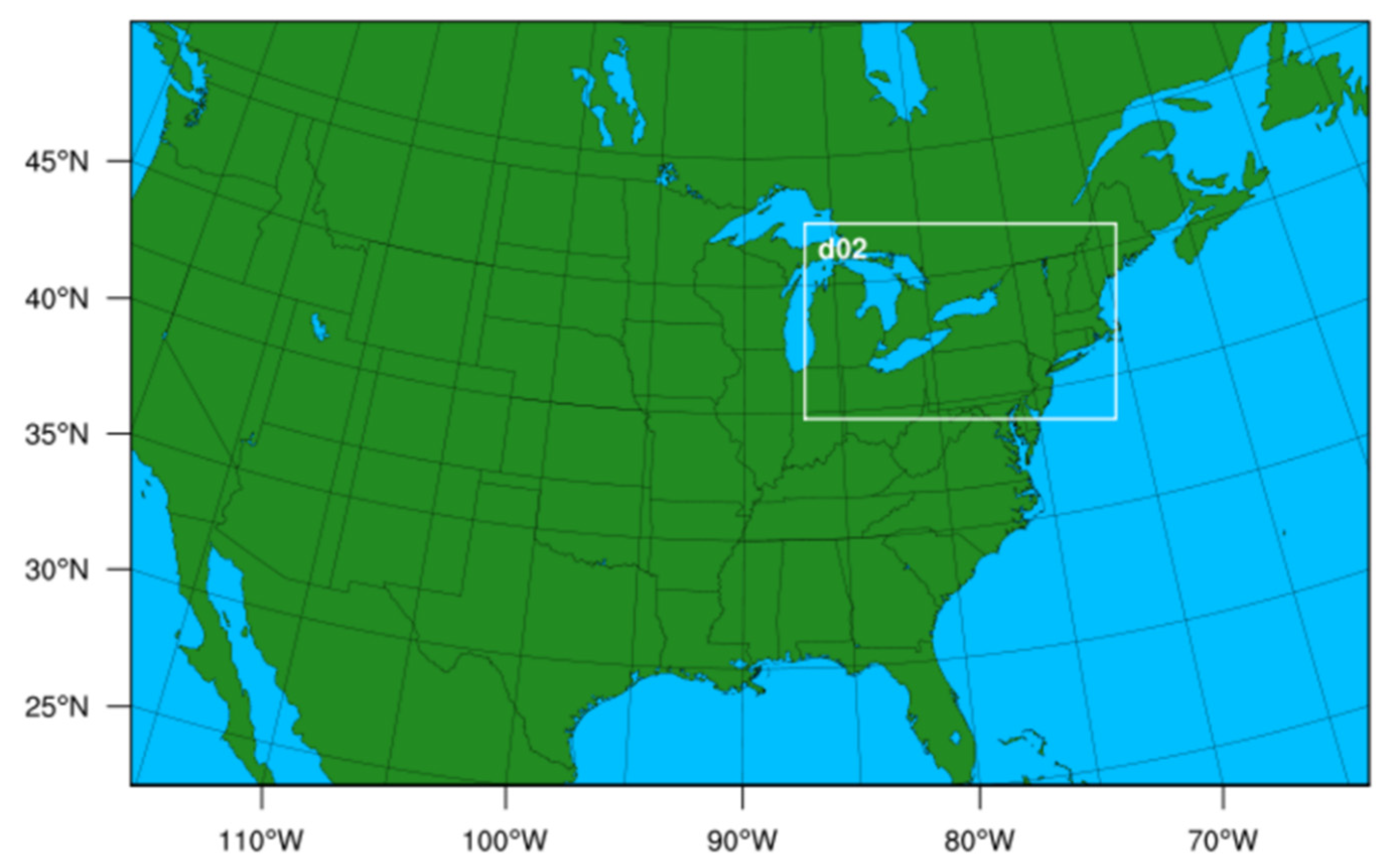
2.3. Numerical Modeling and Case Selection

Given the grid spacing of the NARR (32 km), direct mesoscale analysis from the resulting composite fields was infeasible as LES features, such as banded precipitation, were not resolved at this grid spacing. To resolve these features, we elected to utilize a representative numerical simulation for each cluster that could be done at much smaller grid spacing and could reveal banding structures within the LES composites. However, the composite averaging methodology smoothed out local features that might be important in the development of LES. Rather than simulate directly on the synoptic composites generated from the cluster analysis, one LES constituent case from each cluster was selected that best matched (via silhouette coefficient) its associated LES composite. Specifically, the case with the highest silhouette coefficient value for each cluster was chosen for numerical simulation. The selected events (Table 2) included 27 December 2013 for Cluster 1 (s = 0.634), 2 December 2010 for Cluster 2 (s = 0.584), and 31 January 2007 for Cluster 3 (s = 0.684). The full NARR dataset (all 30 vertical levels) from these three selected cases was used to set initial and boundary conditions in the Advanced Research Weather Research and Forecasting Model (WRF-ARW) version 3.6.1 [32].
The mesoscale simulations of the three selected LES events were done over the same 48 h temporal period as the original composites, using a two-way nested setup with one 15 km parent domain and a 5 km nested domain Figure 5, both with 40 vertical levels. Parameterizations chosen for WRF-ARW runs were largely based on previous studies that successfully utilized WRF-ARW to generate LES [33,34,35]. Table 3 shows a complete list of the parameters used for both domains (no cumulus parameterization was used for the 5 km nested domain). Additionally, a one-dimensional multilayer lake model based on the Community Land Model version 4.5 (CLM 4.5 [36]) was coupled with the WRF-ARW model to improve lake characteristics in the simulations. Finally, improved renderings of the coarse skin temperatures (which approximate lake surface temperatures) were extracted from the Moderate Resolution Imaging Spectroradiometer (MODIS) land-use dataset, which differentiates lake and ocean grid points [37]. The simulations produced fully three-dimensional renderings of the mesoscale conditions in the representative cases retained for further analysis and discussion of the distinctions between the cluster environments.

3. Results and Discussion

3.1. Composite Analysis
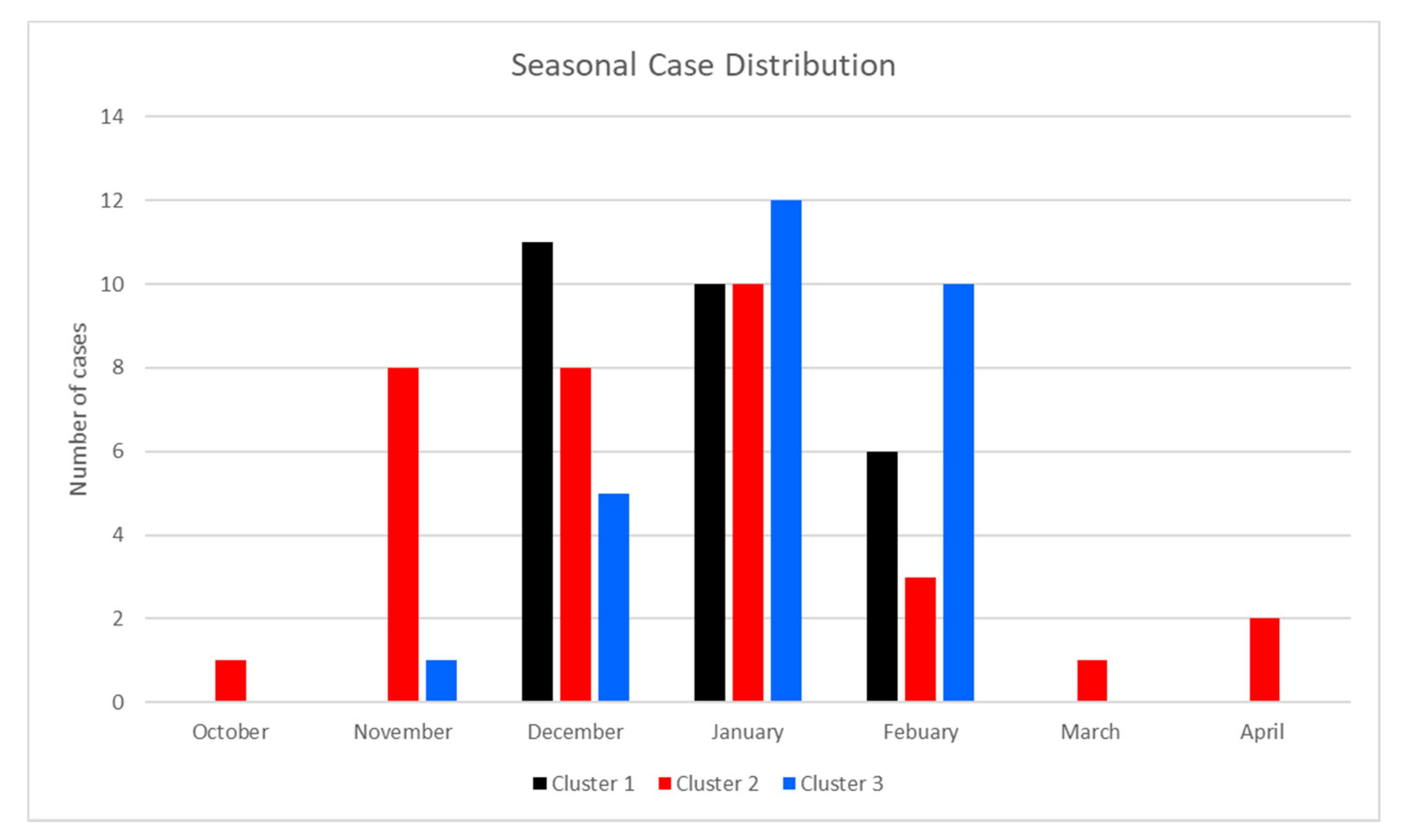
As described previously, three composites were constructed to analyze the different synoptic-scale structures of Lake Erie and Lake Ontario LES events. The synoptic-scale structures of the three composites were like those in References [23,25], showing a mid-level low centered near the Hudson Bay coupled with a surface cyclone northeast of the Great Lakes and a surface anticyclone to the southwest. However, important differences among the synoptic-scale patterns in the clusters produced different mesoscale conditions for the LES in each cluster, as described in the next section.

3.1.1. Cluster 1

Initially, the Cluster 1 composite revealed a positively tilted longwave 500 mb trough over the western Great Lakes basin with associated differential cyclonic vorticity advection (CVA) present over Lakes Erie and Ontario (Figure 6a). CVA is important for strengthening LES via mid-level quasigeostrophic (QG) forcing [3]. Over the following 24 h, the trough propagated southeastward while retaining a neutral tilt, resulting in mostly zonal flow over the lakes. This transition to a neutral tilt produced ridging in the western third of the domain with anticyclonic vorticity advection (AVA) helping to develop a surface anticyclone over the southern Plains (Figure 6d). This trough–ridge pattern helped to establish the necessary LES dipole structure [25] for a favorable westerly/southwesterly surface wind field over both lakes, providing sufficient fetch for a high-impact LES event.

3.1.2. Cluster 2

At the initial analysis time for the Cluster 2 composite, a neutrally tilted longwave trough was located over the western Great Lakes (Figure 7a), contrasting the positively tilted trough from Cluster 1. As in Cluster 1, the trough propagated southeastward and deepened, eventually forming a closed circulation south of James Bay, which resulted in a negative tilt and northwesterly wind shift over the lakes. This upper level pattern resulted in a modification of the surface dipole structure (Figure 7c) relative to expectations [25], producing weak cyclogenesis over the eastern Great Lakes, with the resulting cyclone propagating towards the Canadian Maritimes. That is, this surface cyclone followed the Alberta Clipper track (Figure 7d) depicted in Reference [45], which was shown to generally be associated with the highest central MSLP values in the cyclone center of any synoptic cyclone storm track. This result was evident with the associated differences in central pressure between this cluster’s cyclone (998 mb) and the cyclone in Cluster 1 (975 mb). A weaker (higher geopotential heights) 500 mb low-pressure anomaly and suppressed CVA (as indicated by the lower geopotential height gradient over the lakes) may have factored into why the central pressure was higher in the Cluster 2 surface cyclone. Finally, this cyclone was coupled with a developing anticyclone over the lower Mississippi Valley. The spatial patterns exhibited by this dipole structure have been associated with widespread coverage LES banding events over Lake Erie due to the pure westerly wind flow and the southwest-to-northeast orientation of Lake Erie [14,45]. A visual inspection of radar imagery from the constituent cases (not shown) in this cluster revealed that 63% of the cases showed this widespread coverage banding structure, which was considerably higher than what was seen in Cluster 1 (33%). Interestingly, this surface structure resulted in low-level confluent flow north of Lake Ontario that likely enhanced the vertical motion necessary for LES in that region. Clearly, the differences in positioning in the synoptic-scale features in Cluster 2 resulted in differences in the characters of the LES events that resulted.

3.1.3. Cluster 3

The mid-level field for the Cluster 3 composite showed a positively tilted trough (like Cluster 1) that was evident throughout the upper levels as well (not shown), with the trough axis meridionally oriented over Lake Michigan (Figure 8a) and an upper-level ridge to the west. However, unlike Cluster 1, the upper-level ridge weakened over the time period leading up to the peak LES activity, resulting in a weakening of the differential anticyclonic vorticity advection (DAVA) which in turn weakened the surface anticyclone (Figure 8c). This pattern yielded a strongly northwesterly flow field over the lakes, which is supportive of a widespread coverage banding structure [14,15,45]. Overall, this pattern was like Cluster 1 in terms of the surface dipole pattern, although the horizontal pressure gradient was weaker in Cluster 3 due to the weakening of the surface anticyclone, likely resulting in a less suitable environment for LES. Further, unlike Cluster 2, no pre-existing cyclone was evident over the eastern Great Lakes region at the initial analysis time, but instead the cyclone formed as the trough retained its negative tilt towards the end of the analysis period (Figure 8b,d). These differences resulted in generally weaker surface winds (about 5 m s−1 slower) (Figure 9) for Cluster 3 relative to Cluster 1, which suggests a less favorable environment for LES [46]. However, as with Cluster 2, low-level confluent flow along and north of Lake Ontario likely helped to enhance rising motion (contrasting the wind pattern from Cluster 1 further). Ultimately, the faster trough evolution in Cluster 3 was primarily responsible for the differences seen between its constituent LES events and those of Clusters 1 and 2.

3.1.4. Cluster Differences

As stated above, the major differences between clusters were primarily evident in the surface fields. A Pearson correlation between geopotential height patterns at different isobaric levels revealed strong spatial similarities that were not as robust in MSLP fields (Figure 10). However, the MSLP fields for Clusters 1 and 3 displayed greater similarities (r = 0.904), as evidenced by the positioning and evolution of the dipole structure. Specifically, Clusters 1 and 3 showed a prominent surface cyclone that remained stationary off the northeast coast of the United States, while Cluster 2′s surface cyclone started over the Great Lakes region and propagated northeast towards the location of Cluster 1 and 3′s surface low (following an Alberta Clipper storm track; Figure 11). The surface anticyclones were stronger for Clusters 1 and 3 as well. However, the closer proximity of the surface cyclone to the lakes for Cluster 3 weakened the strength of the low-level pressure gradient and subsequently the wind speeds. The differing position of the dipole structure was most impactful during the first six hours. The surface cyclone present over the Great Lakes associated with Cluster 2 at t = 0 h caused northwesterly flow over Lake Erie and Lake Ontario. This could have an impact on LES development, as air flowing over the lakes will not destabilize as much due to a lack of fetch, often leading to a multiple-band event [14,33]. It should be noted that the pressure gradient, in terms of magnitude and direction, was similar between Clusters 1 and 2, even though the actual pressure values were lower over the lakes for Cluster 2 and the dipole structures were dissimilar.
Although Clusters 1 and 3 exhibited similar spatial structures, there were some differences observed in variable magnitudes of the large-scale systems. The pressure gradient over Lake Erie and Lake Ontario was slightly stronger for Cluster 1, which was attributed to the stronger surface anticyclone in Cluster 1 relative to Cluster 3. Surface wind fields supported this result, showing wind speeds up to 5 m s−1 faster over Lake Erie for Cluster 1 (Figure 9). The shapes of the surface anticyclones in Clusters 1 and 3 also had important differences, particularly in that Cluster 3′s anticyclone had a meridional elongation while Cluster 1′s anticyclone exhibited greater east-to-west (zonal) extent. This shift led to slightly higher surface pressure for Cluster 3 in the study area (roughly 2 mb). These results translated into differences between the mesoscale simulations of the example constituent cases, as shown below.

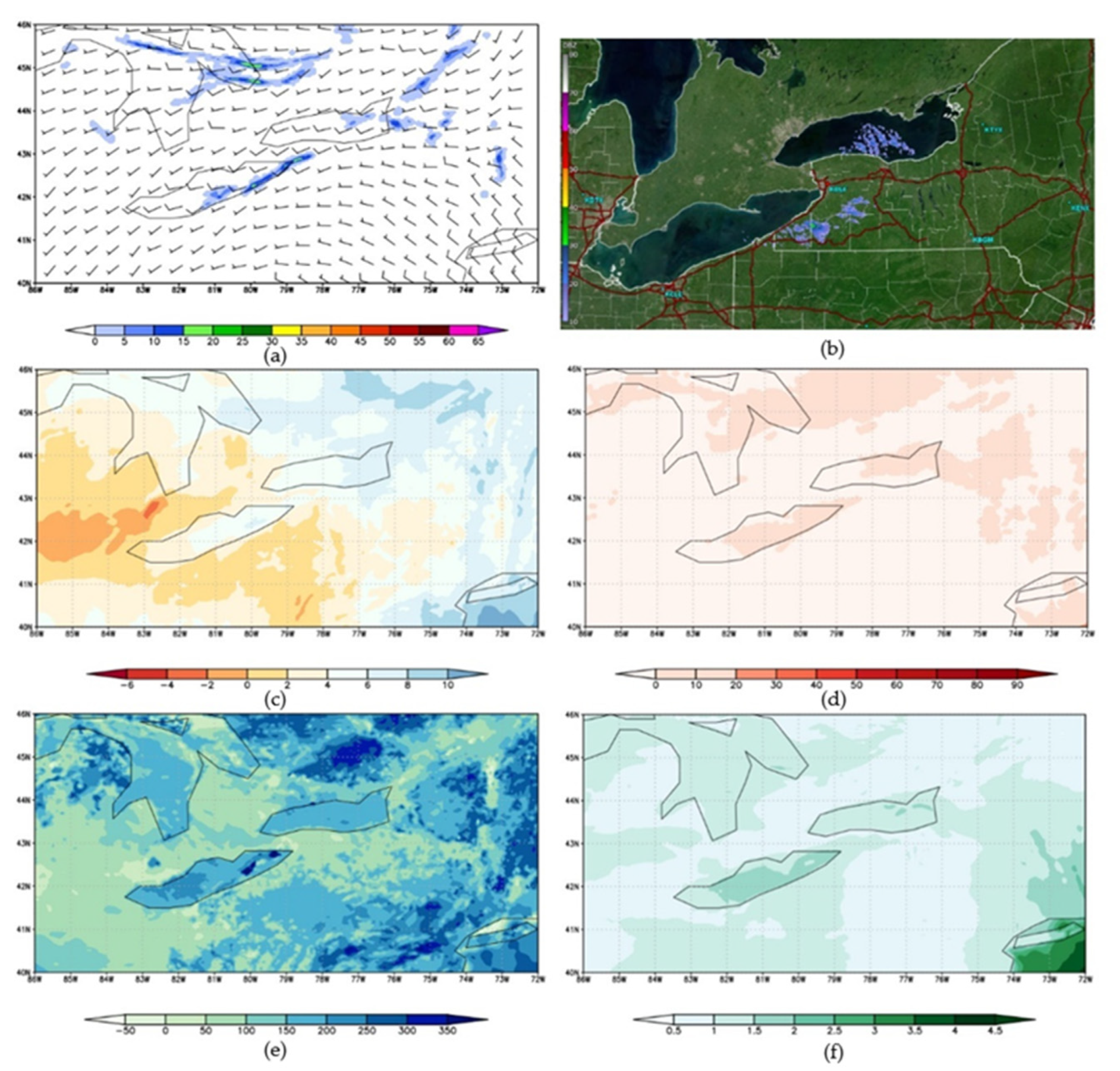
3.2. WRF Simulations

After isolating the dominant synoptic-scale structures, one case from each cluster was selected, based on silhouette coefficient calculations, to assess the mesoscale conditions further. For Cluster 1, 27 December 2013 was selected as its spatial fields were most strongly representative of those within the cluster (s = 0.634). Additionally, for Cluster 2, 2 December 2010 was selected (s = 0.584) and for Cluster 3, 31 January 2007 was selected (s = 0.684). Before analyses of output from WRF were conducted, WSR-88D NEXRAD Level 2 radar data from KBUF (Buffalo, NY, USA) and KTYX (Montague, NY, USA) were retained from each case to assess the representativeness of the spatial precipitation patterns visually. Spatial structure was the primary focus of these evaluations due to uncertainties with reflectivity values associated with overshooting radar beams during these relatively shallow LES events [47]. Overall, the WRF was successfully able to capture the overall spatial features for each of the cases (Figure 12, Figure 13 and Figure 14).

3.2.1. Case 1: 27 December 2013

This event was typical in that LES formed after the passage of a synoptic low-pressure system [23]. Impacts from this event were limited to the lee of Lake Ontario (no LES report was recorded for Erie County). During the event, an LLAP band formed off Lake Ontario at 4:00 p.m. local time and produced as much as 20 inches of snowfall locally, resulting in $9000 in damage [26]. While the WRF did depict the LLAP band successfully, its placement was slightly further south and extended further west across the lake (Figure 12a,b).
The mesoscale conditions characterizing each lake’s impact region differed in the WRF simulations, revealing the causes of the lack of LES off Lake Erie on this day. First, surface–850 mb (hereafter known as low-level) lapse rates were up to 3 °C km−1 steeper over Lake Ontario, which was attributed to higher 850 mb temperatures over Lake Erie (Figure 12c). Lapse rates were calculated in this specific layer (surface–850 mb), as empirical evidence has shown that there must be a minimum 13 °C difference between these two layers to initiate LES formation [14,46,48,49]. The simulated planetary boundary layer (PBL) depth was also slightly greater over Lake Ontario (1.4 km) than over Lake Erie (1.2 km). Surface-based convective available potential energy (CAPE) was much higher over Lake Ontario (up to 70 J kg−1) than over Lake Erie (up to 30 J kg−1) (Figure 12d). Lake Ontario’s sensible heat flux (SHF) values were also much higher (300–350 W m−2) than those over Lake Erie (200–250 W m−2), although latent heat fluxes (LHF) were similar over both lakes (240–270 W m−2; Figure 12e). However, higher moisture (Figure 12f) and a low-level convergence zone (Figure 12a) over Lake Ontario supported the resulting LLAP band, which produced snow over the Tug Hill Plateau region [7,21,50]. A very weak band (<15 dBZ) of precipitation was also generated on the lee side of Lake Erie (Figure 12b), which resulted from a notable convergence zone west of the snowfall area that was lake-influenced, as the rest of the wind field remained uniformly westerly over the lake. These convergent zones are common during LLAP events, resulting from mesolows originating from strong surface thermal gradients between the land and lake [6]. Ultimately, these mesoscale conditions resulted in more pronounced snowfall for Lake Ontario (Figure 12a), which suggested that Cluster 1′s pattern is more suitable for Lake Ontario LES events. This suggests that Case 1′s pattern is more suitable for LES events off Lake Ontario, despite weaker LES bands also occurring off Lake Erie at the same time.

3.2.2. Case 2: 2 December 2010

The Cluster 2 representative case produced severe LES impacts for Erie County, with 42 inches of snowfall and $50,000 in property damage [26]. Like Case 1, LES formed following a departing synoptic system, which manifested in WRF simulations as a band of precipitation. In contrast to Cluster 1′s case, LES activity during this event was confined to Lake Erie’s impact region, as Oswego County did not receive an LES report from this event. However, an extensive area of moderate snowfall was observed in Lake Ontario’s lee (up to eight inches). The lack of LES off Lake Ontario was attributed to elevated wind shear by the NOAA storm database.
The WRF simulation successfully depicted banded convection off Lake Erie, although it also produced less banded precipitation over Lake Ontario’s impact region (Figure 13a). For the WRF simulations, moderate precipitation was generated off both lakes, although more convective organization was observed over Lake Erie, manifested as an LLAP band, while activity over Lake Ontario was more discrete in nature, consistent with radar and observations (Figure 13a,b). The simulated environmental conditions over both lakes showed similar instability and low-level wind fields, helping to reinforce the similarities in simulated reflectivity. Specifically, low-level lapse rates up to 10 °C km−1 (Figure 13c) and surface-based CAPE values of up to 80 J kg−1 (Figure 13d) were observed over both lakes. Surface sensible heat fluxes were similar across both lakes, with SHF and LHF ranging from 100–150 W m−2 and 150–180 W m−2, respectively (Figure 13e). Moisture contents were also similar, although it was slightly higher over Lake Ontario than Lake Erie (Figure 13f). PBL heights ranged from 1.2 to 1.4 km over both lakes, and both lakes had west-southwesterly flow at roughly 10 m s−1 at precipitation onset. This flow pattern likely led to more convective organization off Lake Erie owing to its geographic orientation. Surface convergence in the lee of Lake Erie may have aided LES organization farther inland (Figure 13a) as well.

3.2.3. Case 3: 31 January 2007

For this final representative case (valid for Cluster 3), LES activity was observed off both lakes, beginning 06:00 EST-5 of 31 January 2007, with the heaviest activity initially limited to Lake Ontario’s impact region. Over time, increased wind shear throughout the 1000–800 mb layer (55° based on KBUF 00Z 01 February 2007 sounding) disrupted LES activity over Lake Ontario, while winds became more southerly over Lake Erie producing an LLAP band. The WRF successfully captured this Lake Erie snow band, but failed to capture the initial Lake Ontario activity for reasons described below. This event produced local snowfall totals of up to 36 inches and $8000 in property damage [26].
Unlike the first two cases, WRF did not simulate significant amounts of LES over either of the lakes as the underlying conditions were more statically stable, with low-level lapse rates peaking at only 8 °C km−1 (Figure 14c). These lapse rates were on average 2 °C km−1 steeper over Lake Ontario, but surface temperatures were 2 °C higher over Lake Erie, which may have played a role in more precipitation being simulated over Lake Erie. The steeper lapse rates seen over Lake Ontario resulted from colder 850 mb temperatures (roughly 4 °C). As a result, PBL heights were also appreciably lower (0.3 km–1 km) and more variable, and surface-based CAPE were limited (0–30 J kg−1) (Figure 14d). At the time the snow band formed, winds were southwesterly at 10 m s−1, which led to greater fetch over Lake Erie than Lake Ontario and relatively larger values of sensible and latent heat fluxes (300–350 W m−2) (Figure 14e). Moisture content was also notably less (1.5 g kg−1 compared to Cluster 1 and 2 g kg−1 compared to Cluster 2) in this case than in the other simulated events (Figure 14f). WRF produced a single LLAP band developing over Lake Erie, consistent with radar data, while limited discrete activity was seen over Lake Ontario (Figure 14a).

4. Conclusions

The goal of this project was to update the synoptic climatology of Lake Erie and Lake Ontario LES events by implementing a case-centric clustering methodology (contrasting previous work [23,25]). The climatology was constructed based on a set of 88 unique LES events that impacted near-shore regions off Lake Erie, Lake Ontario, or both. Three LES clusters were derived from NARR reanalysis fields for the LES events, based on the unrotated PCA methodology blended with a k-means cluster analysis. To characterize the mesoscale environments underlying each synoptic-scale cluster, WRF simulations were run on three representative cases (one per cluster). The synoptic-scale composites revealed upper-level structures important for LES that aligned with previous studies [23,24,25]. There were notable discrepancies between the environments when translating the results to surface fields, as confirmed by correlations and direct assessment of the mesoscale conditions portrayed in the representative simulations.
In general, each cluster’s differences can be summarized by noting unique surface level synoptic-scale structures, despite the similarities in the upper levels.
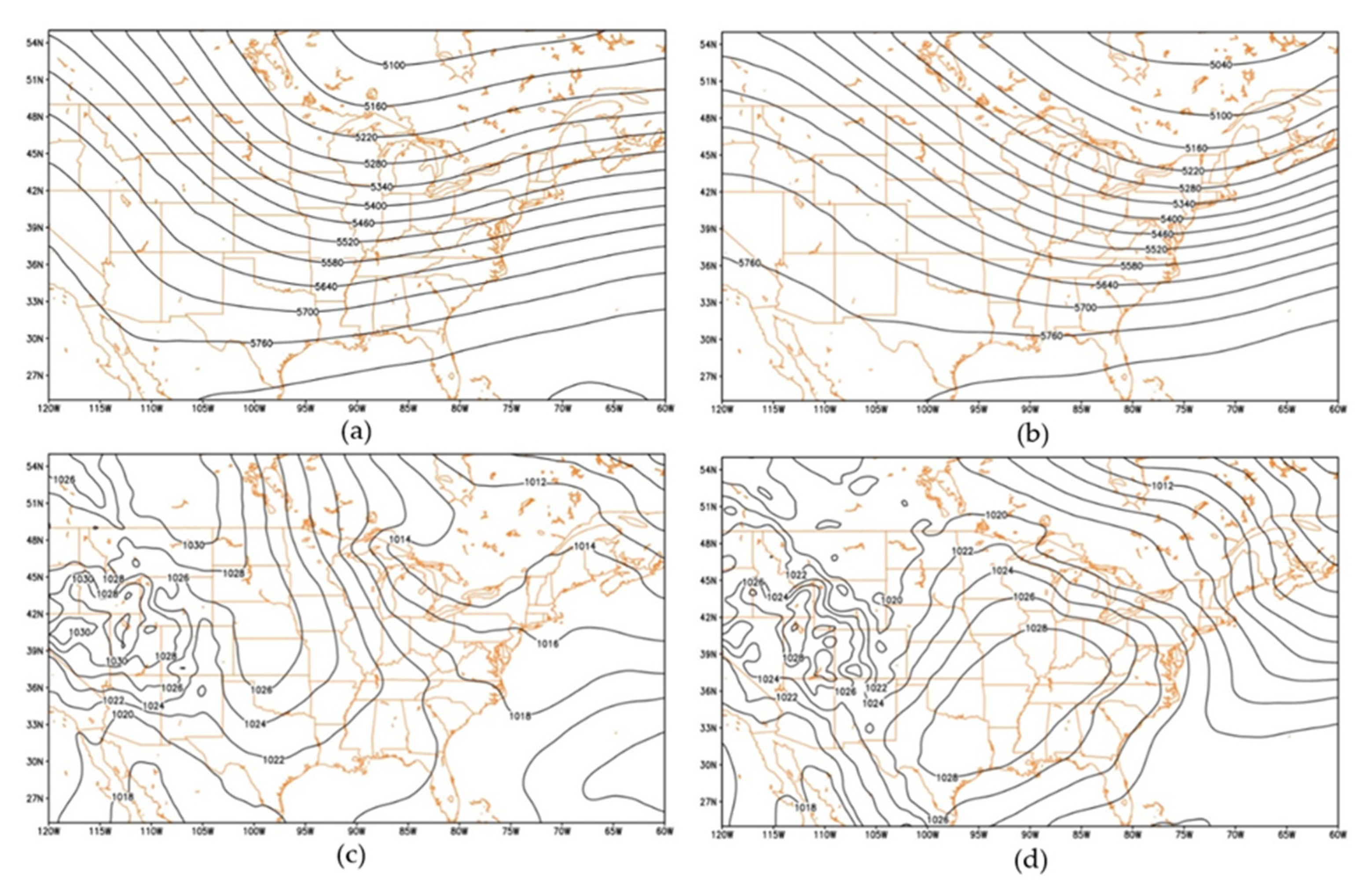
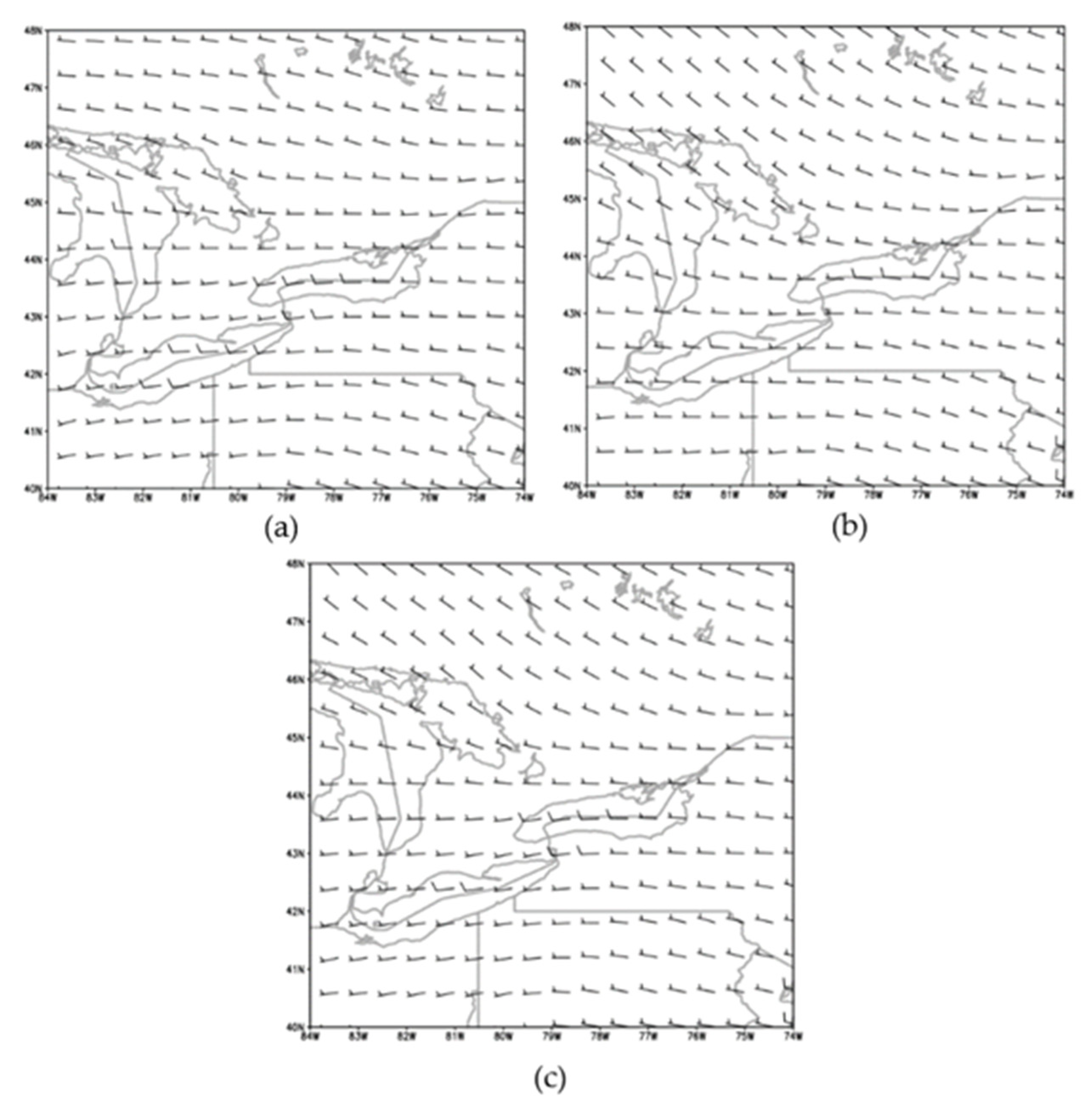
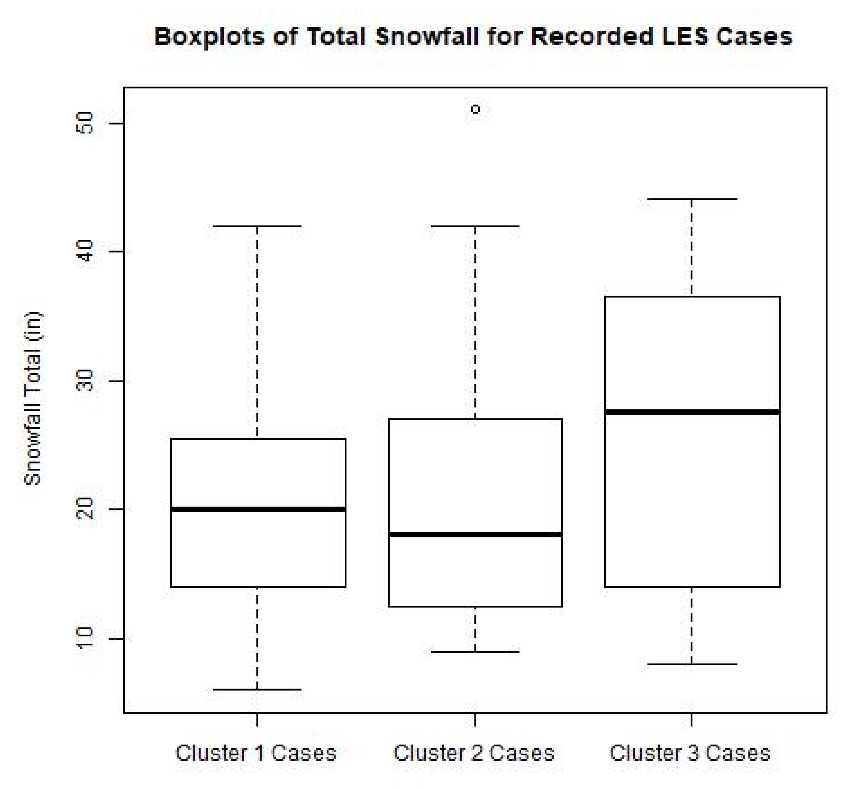
  • Cluster 1—A dipole structure featuring a stationary low-pressure anomaly off the northeast U.S coast and a high-pressure anomaly located over the south central/southeast U.S that originates from the northern Great Plains. Both pressure systems strengthened throughout the study period. The spatial setup of this dipole led to strong west-southwesterly winds that flowed across the long axes of both lakes.
  • Cluster 2—A dynamic dipole featuring cyclogenesis over the Great Lakes following an Alberta Clipper track, and a higher central pressure than any of other the low-pressure systems identified [45]. The high-pressure anomaly features similar spatial structure and evolution to other clusters but is weaker. The spatial structure of the dipole initially results in pure westerly winds over the two lakes. Westerly flow over Lake Erie has been associated with widespread coverage band structure, and events grouped in this cluster exhibited wide coverage characteristics more frequently than any cluster. Although the dipole was weaker, the pressure gradient was of a similar magnitude to Cluster 1, which resulted in similar wind speeds.
  • Cluster 3—A dipole structure similar to Cluster 1 with a few unique distinctions. The dipole structure overall was weaker, consisting of higher central pressure for the low-pressure anomaly and lower pressure for the high-pressure anomaly. The structure of each of the pressure systems differed as well, as the high-pressure anomaly was more elongated and positioned closer to the two lakes. These observations ultimately led to a less conducive LES environment featuring higher surface pressure and slightly slower winds.
Numerical simulations revealed different mesoscale conditions unique to each case. Case 2 featured the most conducive convective environment, with large amounts of instability and atmospheric water vapor content that resulted in substantial LLAP bands over both lakes. The general mesoscale environment was similar for Case 1 except that instability and moisture signals were slightly weaker, particularly over Lake Erie, which manifested in a single LLAP band over Lake Ontario and a widespread coverage band over Lake Erie Figure 14. The stable environment of Case 1 may reflect the influence of the surface anticyclone present in the Cluster 1 composite. The higher surface pressures and close proximity to Lake Erie may have played a role in the suppression of LES activity as surface-based CAPE was near zero over most Lake Erie, surface pressure was 6–10 mb higher, and lapse rates and surface temperatures were 1–3 °C km−1 and 3–6 °C lower over both lakes, respectively (Figure 6, Figure 7, Figure 12 and Figure 13). The Case 3 simulation exhibited the least conducive mesoscale environment, as precipitation fields showed much less coverage that Case 1 or 2, with only a narrow LLAP band being generated over Lake Erie owing to the southwesterly wind profile and subsequent higher energy and moisture fluxes.
Clusters 1 and 2 appeared to be the most conducive to LES for several reasons. Composites and WRF simulations suggested that the underlying synoptic patterns have more of an influence for Cluster 1, while the mesoscale patterns, primarily the stability profile and atmospheric water vapor content, appeared to have more of an influence on Cluster 2. The mesoscale analysis of Cluster 1′s simulation revealed that LES activity was primarily limited to Lake Ontario while the opposite was true for Cluster 2. This result was also seen in the constituent cases, as 60% of LES cases in Cluster 1 were strictly Lake Ontario events and 56% of cases in Cluster 2 were Lake Erie events. This result suggests that Lake Ontario heavy LES events are most influenced by the overlying synoptic scale characteristics, while Lake Erie heavy LES events are primarily governed by underlying mesoscale conditions. This result makes sense given that the smaller bathymetry of Lake Erie increases its susceptibility to rapid changes (such as ice cover onset), which are critical factors governing LES production [5,34]. Minimal activity was observed for Cluster 3, which parallels what was observed in the synoptic analysis, as instability was substantially lower, likely due to the proximity of the anticyclone to the lakes. Interestingly, an analysis of snowfall totals reported from each event revealed that Cluster 3 cases on average produced higher snowfall totals (25.64 in) than those of Clusters 1 (20.81 in) and 2 (21.08 in). Given the impacts of the example case for Cluster 3 (which showed minimal snowfall activity relative to the other two clusters), this result was surprising. However, this was attributed to tremendous variability (IQR of 22.25 in) within the snowfall totals for Cluster 3′s cases (Figure 15), as well as the large number of Lake Ontario cases (75%) that were included in Cluster 3′s case set. This result suggests that Cluster 3′s example case, while best matching the composite based on the silhouette coefficient, is one of several examples of Cluster 3 LES events and is not representative of all of Cluster 3. That is, Cluster 3 appears to be a “catch-all” cluster that included LES events with widely variable impacts. Unfortunately, the best way to categorize this cluster of cases further requires a larger sample size, which may be possible in future work.
Overall, the results of this study allow for better comprehension of the large-scale atmospheric conditions associated with impactful LES storms, which could improve the prediction of these features and possibly reduce their impact. Additionally, these composites form a baseline for comparing synoptic-scale LES events with their associated mesoscale environmental conditions, which could be used in future studies specifically addressing the impacts of warming climate conditions (and warming lakes) on the severity of future LES events. In future work, a similar approach will be used for the remaining Laurentian Great Lakes to assess whether the synoptic set-ups are like those identified in this study. An understanding of the synoptic-scale conditions associated with LES will allow local meteorologists to forecast these events with a greater lead time and more certainty, which will aid in preventing some of the common hazards observed with these storms.

Author Contributions

Conceptualization, A.M. and J.W.; methodology, A.M.; software, J.W.; validation, J.W. and A.M.; formal analysis, J.W.; investigation, J.W.; resources, J.W.; data curation, J.W. and A.M.; writing—original draft preparation, J.W.; writing—review and editing, A.M.; visualization, J.W.; supervision, J.W.; project administration, A.M. All authors have read and agreed to the published version of the manuscript.

Funding

This research received no external funding.

Acknowledgments

We wish to thank two anonymous reviewers for their valuable contributions to help improving this manuscript. We also wish to thank Jamie Dyer and Chris Fuhrmann for support in this research.

Conflicts of Interest

The authors declare no conflict of interest.

References

  1. Hill, J.D. Snow Squalls in the Lee of Lakes Erie and Ontario; NOAA Tech. Memo; NWS ER-43; 1971; p. 20, [NTIS COM-72-00959]. [Google Scholar]
  2. Orlanski, I. A rational subdivision of scales for atmospheric processes. Bull. Am. Meteorol. Soc. 1975, 56, 527–530. [Google Scholar]
  3. Notaro, M.; Zarrin, A.; Vavrus, S.; Bennington, V. Simulation of heavy lake-effect snowstorms across the great lakes basin by RegCM4: Synoptic climatology and variability. Mon. Weather Rev. 2013, 141, 1990–2014. [Google Scholar] [CrossRef]
  4. Wiggin, B.L. Great Snows of the Great Lakes. Weatherwise 1950, 3, 123–126. [Google Scholar] [CrossRef]
  5. Niziol, T.A. Operational Forecasting of Lake Effect Snowfall in Western and Central New York. Weather Forecast. 1987, 2, 310–321. [Google Scholar] [CrossRef]
  6. Steiger, S.M.; Schrom, R.; Stamm, A.; Ruth, D.; Jaszka, K.; Kress, T.; Rathbun, B.; Frame, J.; Wurman, J.; Kosiba, K. Circulations, bounded weak echo regions, and horizontal vortices observed within long-lake-axis-parallel-lake-effect storms by the doppler on wheels. Mon. Weather Rev. 2013, 141, 2821–2840. [Google Scholar] [CrossRef]
  7. Veals, P.G.; James Steenburgh, W. Climatological characteristics and orographic enhancement of lake-effect precipitation east of Lake Ontario and over the Tug Hill Plateau. Mon. Weather Rev. 2015, 143, 3591–3609. [Google Scholar] [CrossRef]
  8. U.S. Census Bureau. 2020: 2019 Census Data. Available online: https://www.census.gov/ (accessed on 21 July 2020).
  9. Changnon, S.A. How a severe winter impacts on individuals. Bull. Am. Meteorol. Soc. 1979, 60, 110–114. [Google Scholar] [CrossRef] [Green Version]
  10. Schmidlin, T.W. Impacts of severe winter weather during December 1989 in the Lake Erie Snowbelt. J. Clim. 1993, 6, 759–767. [Google Scholar] [CrossRef] [Green Version]
  11. Kunkel, K.E.; Westcott, N.E.; Kristovich, D.A.R. Assessment of Potential Effects of Climate Change on Heavy Lake-Effect Snowstorms Near Lake Erie. J. Great Lakes Res. 2002, 28, 521–536. [Google Scholar] [CrossRef]
  12. Mason, L.A.; Riseng, C.M.; Gronewold, A.D.; Rutherford, E.S.; Wang, J.; Clites, A.; Smith, S.D.P.; McIntyre, P.B. Fine-scale spatial variation in ice cover and surface temperature trends across the surface of the Laurentian Great Lakes. Clim. Chang. 2016, 138, 71–83. [Google Scholar] [CrossRef]
  13. Baijnath-Rodino, J.A.; Duguay, C.R.; LeDrew, E. Climatological trends of snowfall over the Laurentian Great Lakes basin. Int. J. Climatol. 2018, 38, 3942–3962. [Google Scholar] [CrossRef]
  14. Niziol, T.A.; Synder, W.R.; Waldstreicher, J.S. Winter Weather Forecasting throughout the Eastern United States. Part IV: Lake Effect Snow. Weather Forecast. 1995, 10, 61–77. [Google Scholar] [CrossRef] [Green Version]
  15. Kristovich, D.A.R.; Laird, N.F. Observations of widespread lake-effect cloudiness: Influences of upwind conditions and lake surface temperatures. Weather Forecast. 1998, 13, 811–821. [Google Scholar] [CrossRef]
  16. Kristovich, D.A.R.; Clark, R.D.; Frame, J.; Geerts, B.; Knupp, K.R.; Kosiba, K.; Laird, N.F.; Metz, N.D.; Minder, J.R.; Sikora, T.D.; et al. The Ontario Winter Lake-Effect Systems field campaign: Scientific and educational adventures to further our knowledge and prediction of lake-effect storms. Bull. Am. Meteorol. Soc. 2017, 98, 315–332. [Google Scholar] [CrossRef]
  17. Byrd, G.P.; Anstett, R.A.; Heim, J.E.; Usinski, D.M. Mobile sounding observations of lake-effect snowbands in western and central New York. Mon. Weather Rev. 1991, 119, 2323–2332. [Google Scholar] [CrossRef] [Green Version]
  18. Cordeira, J.M.; Laird, N.F. The influence of ice cover on two lake-effect snow events over Lake Erie. Mon. Weather Rev. 2008, 136, 2747–2763. [Google Scholar] [CrossRef] [Green Version]
  19. Vavrus, S.; Notaro, M.; Zarrin, A. The role of ice cover in heavy lake-effect snowstorms over the great lakes basin as simulated by RegCM4. Mon. Weather Rev. 2013, 141, 148–165. [Google Scholar] [CrossRef]
  20. Campbell, L.S.; Steenburgh, W.J.; Veals, P.G.; Letcher, T.W.; Minder, J.R. Lake-effect mode and precipitation enhancement over the Tug Hill Plateau during OWLeS IOP2b. Mon. Weather Rev. 2016, 144, 1729–1748. [Google Scholar] [CrossRef]
  21. Rodriguez, Y.; Kristovich, D.A.R.; Hjelmfelt, M.R. Lake-to-lake cloud bands: Frequencies and locations. Mon. Weather Rev. 2007, 135, 4202–4213. [Google Scholar] [CrossRef]
  22. Steiger, S.M.; Hamilton, R.; Keeler, J.; Orville, R.E. Lake-effect thunderstorms in the lower great lakes. J. Appl. Meteorol. Clim. 2009, 48, 889–902. [Google Scholar] [CrossRef] [Green Version]
  23. Ellis, A.W.; Leathers, D.J. A synoptic climatological approach to the analysis of lake-effect snowfall: Potential forecasting applications. Weather Forecast. 1996, 11, 216–229. [Google Scholar] [CrossRef] [Green Version]
  24. Liu, A.Q.; Moore, G.W.K. Lake-effect snowstorms over southern Ontario, Canada, and their associated synoptic-scale environment. Mon. Weather Rev. 2004, 132, 2595–2609. [Google Scholar] [CrossRef]
  25. Suriano, Z.J.; Leathers, D.J. Synoptic climatology of lake-effect snowfall conditions in the eastern Great Lakes region. Int. J. Clim. 2017, 37, 4377–4389. [Google Scholar] [CrossRef]
  26. Storm Events Database. Available online: https://www.ncdc.noaa.gov/stormevents/ (accessed on 4 May 2017).
  27. National Weather Service Instruction 10-1605. Available online: http://www.nws.noaa.gov/directives/sym/pd01016005curr.pdf (accessed on 23 August 2017).
  28. Mesinger, F. North American Regional Reanalysis. Bull. Am. Meteorol. Soc. 2006, 87, 343–360. [Google Scholar] [CrossRef] [Green Version]
  29. Mercer, A.E.; Shafer, C.M.; Doswell, C.A.; Leslie, L.M.; Richman, M.B. Synoptic composites of tornadic and nontornadic outbreaks. Mon. Weather Rev. 2012, 140, 2590–2608. [Google Scholar] [CrossRef] [Green Version]
  30. Wilks, D.S. Statistical Methods in the Atmospheric Sciences; Academic Press: San Diego, CA, USA, 2011; p. 614. [Google Scholar]
  31. Rousseeuw, P.J. Silhouettes: A graphical aid to the interpretation and validation for cluster analysis. J. Comput. Appl. Math. 1987, 20, 53–65. [Google Scholar] [CrossRef] [Green Version]
  32. Skamarock, W.C.; Klemp, J.B.; Dudhia, J.; Gill, D.O.; Barker, D.M.; Wang, W.; Powers, J.G. A Description of the Advanced Research WRF Version 3. NCAR Technical Note-475+ STR. University; Corporation for Atmospheric Research: Boulder, CO, USA, 2008. [Google Scholar] [CrossRef]
  33. Shi, J.J.; Tao, W.K.; Matsui, T.; Cifelli, R.; Hou, A.; Lang, S.; Tokay, A.; Wang, N.Y.; Peters-Lidard, C.; Skofronick-Jackson, G.; et al. WRF simulations of the 20–22 January 2007 snow events over eastern Canada: Comparison with in situ and satellite observations. J. Appl. Meteorol. Clim. 2010, 49, 2246–2266. [Google Scholar] [CrossRef] [Green Version]
  34. Wright, D.M.; Posselt, D.J.; Steiner, A.L. Sensitivity of lake-effect snowfall to lake ice cover and temperature in the great lakes region. Mon. Weather Rev. 2013, 141, 670–689. [Google Scholar] [CrossRef] [Green Version]
  35. Mallard, M.S.; Nolte, C.G.; Bullock, O.R.; Spero, T.L.; Gula, J. Using a coupled lake model with WRF for dynamical downscaling. J. Geophys. Res. Atmos. 2014, 119, 7193–7208. [Google Scholar] [CrossRef]
  36. Oleson, K.W. Technical description of version 4.5 of the Community Land Model (CLM); NCAR Tech. Note NCAR/TN-5031STR; National Center for Atmospheric Research: Boulder, CO, USA, 2013; p. 422. [Google Scholar] [CrossRef]
  37. Wan, Z.; Zhang, Y.; Zhang, Q.; Li, Z.-L. Validation of the land-surface temperature products retrieved from moderate resolution imaging spectroradiometer data. Remote Sens. Environ. 2002, 83, 163–180. [Google Scholar] [CrossRef]
  38. Tao, W.-K.; Simpson, J. Goddard cumulus ensemble model. Part I: Model description. Terr. Atmos. Ocean. Sci. 1993, 4, 35–72. [Google Scholar] [CrossRef]
  39. Mellor, G.L.; Yamada, T. Development of a turbulence closure model for geophysical fluid problems. Rev. Geophys. 1982, 20, 851–875. [Google Scholar] [CrossRef] [Green Version]
  40. Ek, M.B.; Mitchell, K.E.; Lin, Y.; Rogers, E.; Grunmann, P.; Koren, V.; Gayno, G.; Tarpley, J.D. Implementation of Noah land surface model advances in the National Centers for Environmental Prediction operational mesoscale Eta model. J. Geophys. Res. Atmos. 2003, 108, 1–16. [Google Scholar] [CrossRef]
  41. Dudhia, J. Numerical study of convection observed during the Winter Monsoon Experiment using a mesoscale two- dimensional model. J. Atmos. Sci. 1989, 46, 3077–3107. [Google Scholar] [CrossRef]
  42. Mlawer, E.J.; Taubman, S.J.; Brown, P.D.; Iacono, M.J.; Clough, S.A. Radiative transfer for inhomogeneous atmospheres: RRTM, a validated correlated-k model for the longwave. J. Geophys. Res. 1997, 102, 16663–16682. [Google Scholar] [CrossRef] [Green Version]
  43. Kain, J.S.; Fritsch, J.M. The role of the convective ‘‘trigger function’’ in numerical prediction of mesoscale convective systems. Meteorol. Atmos. Phys. 1993, 49, 93–106. [Google Scholar] [CrossRef]
  44. Janjic, Z.I. The surface layer in the NCEP Eta Model. In Eleventh Conference on Numerical Weather Prediction, Norfolk VA, USA, 19–23 August 1996; American Meteorological Society: Boston, MA, USA, 1996; pp. 354–355. [Google Scholar]
  45. Mercer, A.E.; Richman, M.B. Statistical differences of quasigeostrophic variables, stability, and moisture profiles in North American storm tracks. Mon. Weather Rev. 2007, 135, 2312–2338. [Google Scholar] [CrossRef] [Green Version]
  46. Sousounis, P.J. Lake-Effect Storms. In Encyclopedia of Atmospheric Sciences; Academic Press: Cambridge, MA, USA, 2001; pp. 1104–1115. [Google Scholar]
  47. Brown, R.A.; Niziol, T.A.; Donaldson, N.R.; Joe, P.I.; Wood, V.T. Improved detection using negative elevation angles for mountaintop WSR-88Ds. Part III: Simulations of shallow convective activity over and around Lake Ontario. Weather Forecast. 2007, 22, 839–852. [Google Scholar] [CrossRef]
  48. Holroyd, E.W. Lake-effect cloud bands as seen from weather satellites. J. Atmos. Sci. 1971, 28, 1165–1170. [Google Scholar] [CrossRef] [Green Version]
  49. Cooper, K.A.; Hjelmfelt, M.R.; Derickson, R.G.; Kristovich, D.A.R.; Laird, N.F. Numerical simulation of transitions in boundary layer convective structures in a lake-effect snow event. Mon. Weather Rev. 2000, 128, 3283–3295. [Google Scholar] [CrossRef]
  50. Hartnett, J.J.; Collins, J.M.; Baxter, M.A.; Chambers, D.P. Spatiotemporal snowfall trends in central New York. J. Appl. Meteorol. Clim. 2014, 53, 2685–2697. [Google Scholar] [CrossRef]
Figure 1. Satellite image of various LES-band types over the Great Lakes basin on 31 December 2017 gathered by the Moderate Resolution Imaging Spectroradiometer (MODIS) on the National Aeronautics and Space Administration’s (NASA) Aqua satellite. A moisture channel via strong long-lake-axis bands over Lake Huron (A) led to the development of widespread coverage bands over Lake Erie (C). Widespread coverage bands were generated over Lake Ontario (B) and Lake Superior (E), as well as a mesoscale vortex over southern Lake Michigan (D).
Atmosphere 11 00872 g001
Figure 2. Map of New York highlighting Erie (left) and Oswego (right) counties; counties are labeled and highlighted with blue hatching.
Atmosphere 11 00872 g002
Figure 3. Scatterplot of the first two principal component (PC) loading vectors, with black dots representing Cluster 1 cases, red squares representing Cluster 2 cases, and blue crosses representing Cluster 3 cases. The separation of cases between the different clusters indicates that the cases were distinguishable and appropriately organized between the three clusters.
Atmosphere 11 00872 g003
Figure 4. Histogram of the seasonal case distribution between the three different clusters.
Atmosphere 11 00872 g004
Figure 5. Domain configuration used for the WRF simulations. Horizontal resolutions for the parent domain and the nested domain (d02) were 15 and 5 km, respectively.
Atmosphere 11 00872 g005
Figure 6. Composite 500 mb geopotential heights (m) for Cluster 1 at the initial timestep (t = 0 h; panel (a)) and the end time (t = 42 h) for the LES event as defined by the NOAA storm event database panel (b), with mean sea-level pressure (MSLP) (mb) at the t = 0 h panel (c) and t = 42 h panel (d).
Atmosphere 11 00872 g006
Figure 7. Composite 500 mb geopotential heights (m) for Cluster 2 at the initial timestep (t = 0 h; panel (a)) and the end time (t = 42 h) for the LES event as defined by the NOAA storm event database panel (b), with mean sea-level pressure (MSLP) (mb) at the t = 0 h panel (c) and t = 42 h panel (d).
Atmosphere 11 00872 g007
Figure 8. Composite 500 mb geopotential heights (m) for Cluster 3 at the initial timestep (t = 0 h; panel (a)) and the end time (t = 42 h) for the LES event as defined by the NOAA storm event database panel (b), with mean sea-level pressure (MSLP) (mb) at the t = 0 h panel (c) and t = 42 h panel (d).
Atmosphere 11 00872 g008
Figure 9. Surface wind fields (m s−1) for Cluster 1 (a), Cluster 2 (b), and Cluster 3 (c), valid for the end time (t = 42 h) for each composite.
Atmosphere 11 00872 g009
Figure 10. Average Pearson correlation coefficients between each listed spatial field for all three clusters, valid for all times in the composite LES event.
Atmosphere 11 00872 g010
Figure 11. MSLP differences (mb) between Cluster 1 and 2 composites at the LES end time (t = 42 h). Note the positive pressure differences recorded over the northeast United States coast and the lower pressure differences located further northeast, indicating the positions of each of the surface cyclones. The Cluster 2 cyclone was associated with the positive pressure differences while the Cluster 1 cyclone was associated with the negative pressure differences.
Atmosphere 11 00872 g011
Figure 12. Composite reflectivity (dBZ) and surface winds (m s−1) (a), KTYX radar data (dBZ) (b), low-level lapse rate (°C km−1) (c), surface-based CAPE (J kg−1) (d), sensible heat flux (W m–2) (e), and specific humidity (g kg−1) (f) as simulated by WRF for Case 1.
Atmosphere 11 00872 g012
Figure 13. Composite reflectivity (dBZ) and surface winds (m s−1) (a), KBUF radar data (dBZ) (b), low-level lapse rate (°C km−1) (c), surface-based CAPE (J kg−1) (d), sensible heat flux (W m–2) (e), and specific humidity (g kg−1) (f) as simulated by WRF for Case 2.
Atmosphere 11 00872 g013
Figure 14. Composite reflectivity (dBZ) and surface winds (m s−1) (a), KBUF radar data (dBZ) (b), low-level lapse rate (°C km−1) (c), surface-based CAPE (J kg−1) (d), sensible heat flux (W m–2) (e), and specific humidity (g kg−1) (f) as simulated by WRF for Case 3.
Atmosphere 11 00872 g014
Figure 15. Boxplots of recorded snowfall totals for all LES cases identified using the NOAA Storm Database, divided by associated cluster.
Atmosphere 11 00872 g015
Table 1. Variance explained for PCs 2 through 6 and silhouette coefficients while using three clusters.
PC 2PC 3 PC 4PC 5PC 6
Individual Variance Explained9.36%7.56%6.11%5.40%4.31%
Cumulative Variance Explained20.3%27.86%33.97%39.37%43.68%
Silhouette Coefficient using Three Clusters0.400.290.230.180.15
Table 2. Three cases used for each WRF run. All information provided about the cases came from the NOAA Storm Events Database. All times are in Eastern Standard Time (EST-5).
Cluster 1Cluster 2Cluster 3
Event Start2013-12-26 16:00 2010-12-01 15:002007-01-31 06:00
Event End2013-12-27 11:00 2010-12-02 19:00 2007-01-31 16:00
Duration19 h28 h10 h
SourceLake OntarioLake ErieLakes Erie and Ontario
Band TypeLLAPLLAPLLAP
Highest Snowfall Total Recorded (in)204235
WRF Simulation Duration48 h48 h48 h
Table 3. Parameterization schemes used in all WRF projections for all domains.
ParameterizationScheme/Model
MicrophysicsGoddard microphysics scheme [38]
Planetary Boundary LayerMellor–Yamada–Janjic [39]
Land Surface ModelNoah Land Surface Model [40]
Shortwave Radiation PhysicsDudhia shortwave scheme [41]
Longwave Radiation PhysicsRapid Radiative Transfer Model [42]
Cumulus SchemeKain–Fritsch * [43]
Surface Layer PhysicsEta similarity [44]
* Note that no cumulus scheme was used for the 5 km nested domain.

