A Hydrodynamical Atmosphere/Ocean Coupled Modeling System for Multiple Tropical Cyclones

Abstract

The goal of this paper is to introduce a new multi-storm atmosphere/ocean coupling scheme that was implemented and tested in the Basin-Scale Hurricane Weather Research and Forecasting (HWRF-B) model. HWRF-B, an experimental model developed at the National Oceanic and Atmospheric Administration (NOAA) and supported by the Hurricane Forecast Improvement Program, is configured with multiple storm-following nested domains to produce high-resolution predictions for several tropical cyclones (TCs) within the same forecast integration. The new coupling scheme parallelizes atmosphere/ocean interactions for each nested domain in HWRF-B, and it may be applied to any atmosphere/ocean coupled system. TC forecasts from this new hydrodynamical modeling system were produced in the North Atlantic and eastern North Pacific from 2017–2019. The performance of HWRF-B was evaluated, including forecasts of TC track, intensity, structure (e.g., surface wind radii), and intensity change, and simulated sea-surface temperatures were compared with satellite observations. Median forecast skill scores showed significant improvement over the operational HWRF at most forecast lead times for track, intensity, and structure. Sea-surface temperatures cooled by 1–8 °C for the five HWRF-B case studies, demonstrating the utility of the model to study the impact of the ocean on TC intensity forecasting. These results show the value of a multi-storm modeling system and provide confidence that the multi-storm coupling scheme was implemented correctly. Future TC models within NOAA, especially the Unified Forecast System’s Hurricane Analysis and Forecast System, would benefit from the multi-storm coupling scheme whose utility and performance are demonstrated in HWRF-B here.

1. Introduction

Sea surface temperatures (SSTs) and interactions between the ocean and atmosphere are critical components for forecasting the genesis and intensity changes of a tropical cyclone (TC). TCs do not usually form if the SSTs are colder than 26 °C [1]. Several observational and numerical studies have demonstrated the existence of important positive and negative feedback mechanisms between the ocean and TCs [2,3,4]. On one hand, increased surface winds enhance turbulent heat flux rates, thereby contributing a positive feedback to intensification. On the other hand, the ocean response to strong hurricane winds can cool the sea surface, thus providing a negative feedback to intensification. Storm-induced surface cooling from 1 to 6 °C has been reported [5]. Bender et al. [6] noted average cooling values of 5.38, 3.58, and 1.88 °C for slow, medium, and fast-moving storms, respectively, and similar cooling for different translation speeds was found in idealized experiments [7].

Using a coupled atmosphere/ocean hurricane model, Bender et al. [6] investigated TC interactions with the ocean. They found that the cooling of the sea surface induced by the TC resulted in a significant impact on the ultimate storm intensity due to the reduction of net heat flux into the TC over regions of decreased SST. The sea surface cooling under a hurricane is primarily a result of vertical turbulent mixing in the ocean, induced by enhanced shear. Other mechanisms that contribute to surface cooling are the upwelling of cooler water from the thermocline to the sea surface due to Ekman pumping (wind stress curl), whose importance for slow-moving storms has been shown by studies like Price [8] and Yablonsky and Ginis [9]; interaction with cold-core ocean vortices [10]; and, paradoxically, advection due to the presence of a warm-core ocean vortices [11], as well as other potential effects in the presence of shallow seafloor topography. The degree of surface cooling is strongly dependent on the initial ocean mixed layer depth, particularly in the presence of oceanic vortices [12].

These effects can only be appropriately simulated with forcing from the atmosphere; this, in turn, requires an adequate simulation of atmosphere/ocean feedback, i.e., coupling between the atmosphere and ocean. The numerical modeling studies of Bender and Ginis [13] have shown that ocean coupling is important for accurate TC intensity predictions, especially for slow-moving storms. They noted that intensity forecasts for Hurricanes Felix, Fran, Opal, and Gilbert significantly improved when the effects of atmosphere/ocean interactions were included in their numerical models.

More recently, atmosphere/ocean coupling has been implemented in high-resolution numerical models. One such model is the Hurricane Weather Research and Forecasting (HWRF) model, which was developed by the National Oceanic and Atmospheric Administration (NOAA)/National Weather Service (NWS)/National Centers for Environmental Prediction (NCEP) and collaborative community partners. HWRF provides important forecast guidance to TC forecast centers around the world [14,15,16,17,18,19,20]. Over the last decade, HWRF has become more sophisticated, with the addition of ocean coupling to simulate critical air–sea interactions and with high-resolution grids that produce increasingly accurate intensity forecasts by resolving convection and TC inner core structure. In fact, Cangialosi [21] found that the operational HWRF is one of the most accurate intensity forecast models evaluated by the NOAA National Hurricane Center (NHC).

Despite these improvements, the operational HWRF system is storm-centric and only simulates one TC at high resolution per forecast integration. To address this shortcoming, a version of HWRF capable of producing multi-storm forecasts, called Basin-Scale HWRF (HWRF-B), was developed at NOAA’s Atlantic Oceanographic and Meteorological Laboratory (AOML) in collaboration with NOAA’s Environmental Modeling Center and the Developmental Testbed Center. HWRF-B is unique in the fact that it can support multiple storm-following nests to produce high-resolution predictions for several TCs within the same forecast integration [22,23]. In general, multi-storm interactions can be separated into three categories: (1) binary for storms in close proximity, (2) intermediate (or outflow) for storms that are interacting with the same synoptic environment, and (3) remote interactions for storms in different ocean basins [23]. Apart from simultaneous high-resolution simulations of several coexisting TCs, the advantages of multi-storm forecasting with a large model domain include a better capability to simulate intermediate and remote interactions between TCs and lower dependence on lateral boundary conditions [24].

With support from the Hurricane Forecast Improvement Program (HFIP) [25,26], HWRF-B has been upgraded annually since 2013 to be as similar in configuration to the operational HWRF as possible. Thus, when any persistent HWRF-B forecast improvements over the operational HWRF are observed, they can reasonably be ascribed to the above-listed advantages of multi-storm simulations. Furthermore, HWRF-B provides a computationally efficient configuration for TC forecasting (i.e., only one initialization is required instead of several) that could produce high-resolution TC forecasts in global models. A recent endeavor in HWRF-B development was to couple the atmosphere model with an ocean model for multiple TCs at high resolution. For this purpose, a new coupling scheme was developed, with special attention paid to efficiency (i.e., virtually no coupling overhead compared to the standalone atmosphere model) and the accuracy of surface field interpolation, which is especially important near sea/land boundaries.

The goals of this manuscript are to introduce the multi-storm coupling scheme used in HWRF-B and to evaluate the resulting TC forecast performance of HWRF-B. Section 2 describes the HWRF-B modeling system, its configuration, and its components. In Section 3, the TC forecast performance of HWRF-B is evaluated. Case studies are presented in Section 4 to examine SST forecasts from the coupled HWRF-B system. Section 5 presents conclusions and a discussion of how this multi-storm coupling technology extends beyond HWRF-B.

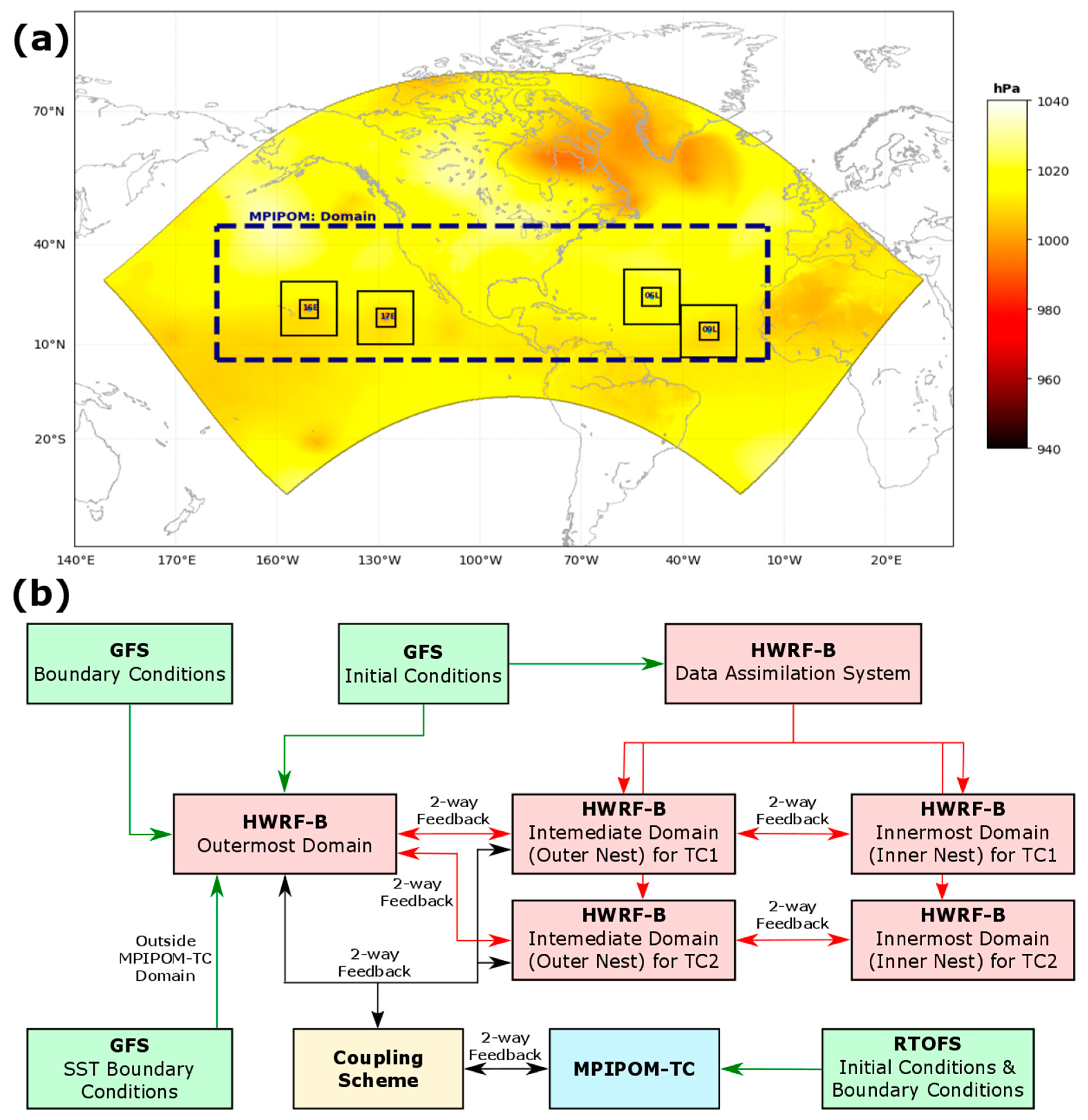
2. Models and Methods

2.1. Atmosphere Model

HWRF-B is a regional dynamical numerical weather prediction modeling system that is capable of producing high-resolution forecasts for coexisting TCs in the same forecast integration. The 2020 version of HWRF-B utilizes basic configuration options identical to the operational HWRF (see next paragraph) and, additionally, includes two advanced configuration options (see Figure 1a): (i) a large, fixed outermost atmospheric domain that spans the eastern North Pacific and North Atlantic hurricane basins (i.e., the entire NHC area of responsibility); and (ii) up to five multiple movable, multi-level nests [22]. The outermost domain covers approximately a quarter of the globe (from 150° E eastward to 30° E and from 35° S to 80° N) and has a horizontal grid spacing of 13.5 km. Two telescopic, storm-following nests are centered on each TC: the outer nest (i.e., intermediate domain) has a size of 16.5° by 16.5° with horizontal grid spacing of 4.5 km and the inner nest (i.e., innermost domain) has a size of 5.5° by 5.5° with horizontal grid spacing of 1.5 km. Previous work has shown the benefits of the advanced configuration options in HWRF-B to improve track forecast guidance [23,24]. By contrast, the operational HWRF is configured with a much smaller outermost domain and high-resolution nests for only one storm per forecast. All domains are two-way interactive, meaning the synoptic-scale is impacted by the vortex-scale and vice versa (Figure 1b).

HWRF-B and HWRF are otherwise identical in atmospheric configuration. HWRF-B uses the Non-hydrostatic Mesoscale Model (NMM) dynamical core [27] and is configured with a rotated latitude-longitude coordinate system on an Arakawa E-grid. The model has 75 hybrid pressure-sigma vertical levels and a model top of 10 hPa. The 2020 version of HWRF-B is configured with an advanced suite of physical parameterizations that are capable of simulating both large and small spatial scales. The microphysics parameterization is the Ferrier-Aligo microphysics scheme, which is a modified version of the tropical Ferrier microphysics scheme based on the Eta Grid-Scale Cloud and Precipitation scheme [28,29]. The cumulus parameterization is the Scale-Aware Simplified Arakawa-Schubert (SASAS) scheme [30,31,32]. The surface-layer parameterization over water in HWRF-B is based on Kwon et al. [33], Powell et al. [34], and Black et al. [35]. The land-surface model is the Noah LSM, broadly used by the NCEP and WRF community [36,37,38,39,40,41,42,43]. The planetary-boundary layer parameterization is the non-local Hybrid Eddy-Diffusivity Mass-Flux (Hybrid EDMF) scheme, where a mass flux approach is used to represent non-local mixing under convective conditions [44,45,46]. The atmospheric radiation parameterizations are the RRTMG shortwave and longwave radiation schemes [47,48]. For more detail, please refer to the documentation for HWRF v4.0a [49].

In all nested domains, a vortex initialization procedure is applied to generate a more realistic TC vortex structure [49,50]. The initial vortex for HWRF-B comes from NCEP’s Global Forecast System (GFS). Depending on the intensity of the TC and the existence of a previous forecast, HWRF-B vortex initialization replaces the initial vortex with one of the following vortices after correcting for intensity and structure: the previous 6 h HWRF-B forecast, a bogus vortex based on a composite of historical TCs, or the original GFS vortex. Furthermore, the initial vortex is improved by assimilating satellite, airborne, and ground-based observations using a hybrid ensemble-variational system based on Gridpoint Statistical Interpolation (GSI) [51,52]. When airborne tail Doppler radar observations are available for a particular TC, an ensemble of 40 HWRF-B members produces error covariances for use in GSI [53,54]. Otherwise, HWRF-B GSI uses covariances from a GFS ensemble that is always available.

2.2. Ocean Model

The storm-centric operational HWRF has used the Message Passing Interface Princeton Ocean Model for Tropical Cyclones (MPIPOM-TC) as its oceanic component for several years. MPIPOM-TC is based on the three-dimensional, primitive equation ocean model known as the Princeton Ocean Model [55]. MPIPOM-TC is computationally efficient and scalable, with netCDF input and output. In addition, MPIPOM-TC supports initialization from a variety of global ocean products. The model description of MPIPOM-TC can be found in Yablonsky et al. [56]. The atmosphere–ocean coupling capabilities of the operational HWRF have been extended to HWRF-B. The MPIPOM-TC is configured for a domain bounded in latitude from 5° N to 45° N and in longitude from 178° W to 15° W with horizontal resolution 1/12° (see Figure 1a). Outside of the MPIPOM-TC domain, HWRF-B ingests constant SST from the GFS Analysis (Figure 1b). Unlike HWRF-B, MPIPOM-TC does not use a rotated grid, which requires special care when coupling these models (see Section 2.3). MPIPOM-TC uses terrain-following sigma vertical coordinates (𝞂) [57]. In the coupled HWRF-B, MPIPOM-TC has 40 full 𝞂-levels from the sea surface to the seafloor, with higher vertical resolution in the region of the main mixed layer and upper thermocline. The 𝞂-levels are 0.0, 0.0009, 0.0018, 0.0029, 0.0042, 0.0056, 0.0073, 0.0091, 0.0113, 0.0136, 0.0164, 0.0196, 0.0233, 0.0273, 0.032, 0.0373, 0.0433, 0.0502, 0.0582, 0.0671, 0.0775, 0.0891, 0.1024, 0.1176, 0.1349, 0.1545, 0.1771, 0.2027, 0.232, 0.2653, 0.3033, 0.3465, 0.396, 0.4524, 0.5164, 0.5896, 0.6729, 0.768, 0.8764, 1.0 with 𝞂 = 0 at the surface and 𝞂 =1 at the bottom. The maximum ocean depth for the current configuration is 5500 m. The level placement is scaled based on the bathymetry of the ocean at a given location; the largest vertical spacing occurs at the maximum ocean depth. The model has a closed boundary condition at the coastline based on a land–sea mask that is consistent with the atmosphere model.

The ocean model is initialized from the NCEP Global Real-Time Ocean Forecast System (RTOFS), based on the HYbrid Coordinate Ocean Model (HYCOM) [58]. A computationally efficient preprocessing procedure for MPIPOM-TC, based on RTOFS data, has been developed for HWRF-B. The temperature and salinity fields are extracted from RTOFS data and then they are horizontally interpolated into the ocean model domain (see Figure 1). RTOFS depth data is also used to construct bottom topography for MPIPOM-TC. In the ocean initialization step, MPIPOM-TC is run for two model days without any wind forcing to spin up currents that are dynamically consistent with the temperature and salinity fields [59].

2.3. Coupling Scheme

During a forecast, a new multi-storm coupling scheme supplies HWRF-B, the atmosphere model (AM), and MPIPOM-TC, the ocean model (OM), each with ocean surface boundary conditions computed by the other component model of the coupled system. Since the coupling scheme is applicable not only to HWRF-B and MPIPOM-TC, but to a broad variety of AM/OM systems, the description of this scheme is provided in general terms below.

Only the AM outermost (stationary) domain and the intermediate (moving) nest domain(s) directly exchange data with the OM via the coupling scheme. Each AM innermost nest domain receives the required OM data via interpolation from its parent intermediate domain. The rationale is that the resolution of the AM innermost domain grid(s) is typically much higher than that of the OM grid, so a direct data exchange between an AM innermost domain and the OM would be of no benefit for either model component of the coupled system and would result in an unnecessary decrease of computational efficiency. This transfer between the AM and OM is represented in Figure 1b.

On each time step of the coupled time integration, the OM sends its instantaneous SST fields to the AM, and these data are used by the AM surface boundary layer scheme as a lower boundary condition. At the same time, the AM supplies the OM with surface heat (long- and shortwave radiation, sensible and latent heat) and momentum fluxes, time-averaged over the last completed coupling time step. The time averaging ensures heat and momentum conservation for the AM-to-OM flux transmission. The flux data are used in the OM surface boundary layer as upper boundary conditions. For the exchange of data between the AM and OM, only ocean grid-point values used as data over land are not relevant to AM/OM coupling.

While the data sent from the OM to the AM belong to the current coupling time step, the fields transmitted from the AM to the OM are obtained from the preceding coupling time step. For the first time step of the forecast, flux values of zero are assumed by the AM. This allows each component model to avoid waiting for its boundary conditions to arrive. As a result, there is no coupling overhead in the numerical time integration, and the speed of the coupled forecast equals the speed of an independent, uncoupled forecast produced by the slower of the two component models (assuming the same number of processors).

The data exchange between the AM and the OM requires interpolation from one grid (grid 1) to the other (grid 2). The interpolation scheme is designed for general grids 1 and 2 which are defined by grid point coordinates; each grid cell is assumed to be quadrilateral. A bilinear interpolation is used, replaced by a linear or a nearest-neighbor interpolation wherever the number of grid 1 cell vertices available for interpolation to a grid 2 point lying inside that cell, is less than the total number of that cell’s vertices (four for a quadrilateral grid). Since the coupling operates with sea surface data, only sea grid point values are considered available for interpolation to the other grid. For an AM grid point close to a sea–land boundary, if there are no OM SST values available for interpolation, a “creeping extrapolation” algorithm is used, with a weighted blend of both the extrapolated values and the default SST values prescribed on the AM grid. The latter values are those used in the AM when it is run standalone; typically, they are initial conditions for SST on the AM grid.

The coupling interpolation requires a pre-forecast initialization, i.e., computation of interpolation weights. A direct computation of the weights includes a search for the grid 1 cell that contains each grid 2 point. The search requires order of magnitude N² operations, where N is the number of grid points; in the case of forecast-specific domains, this is too slow. An algorithm based on scanning of grid 2 along a continuous path was developed and implemented in the coupled system; this allows the scheme to reduce the number of operations to the order of N^3/2, which renders the computation cost of the search algorithm negligible.

For data exchange with the OM grid, the AM nest grids are considered moving sections of a single AM grid that has the same resolution as AM nest grids and is the size of the entire AM parent domain. This avoids re-initializing the interpolation each time a nest moves and applies generally to any model with one or more moving nests.

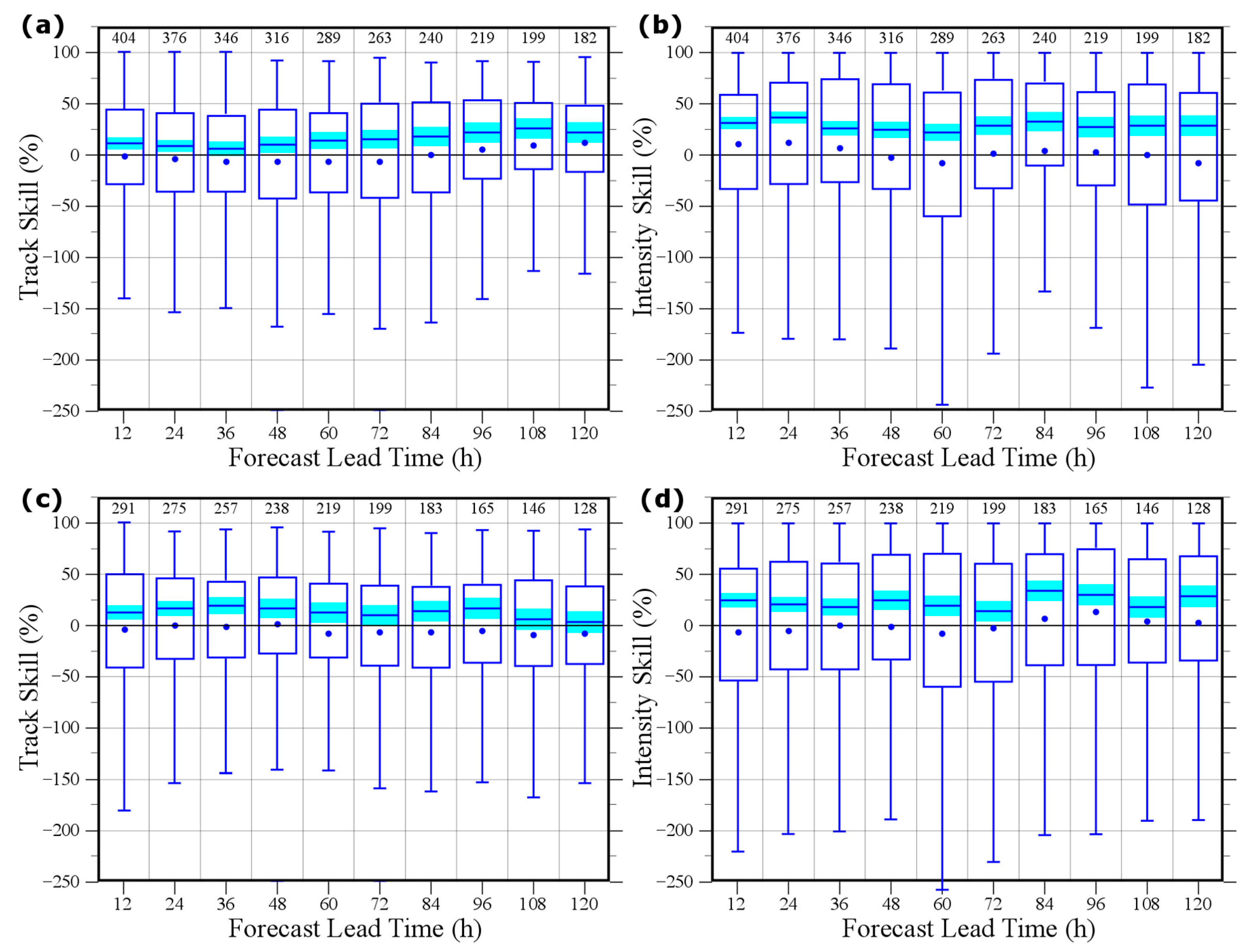
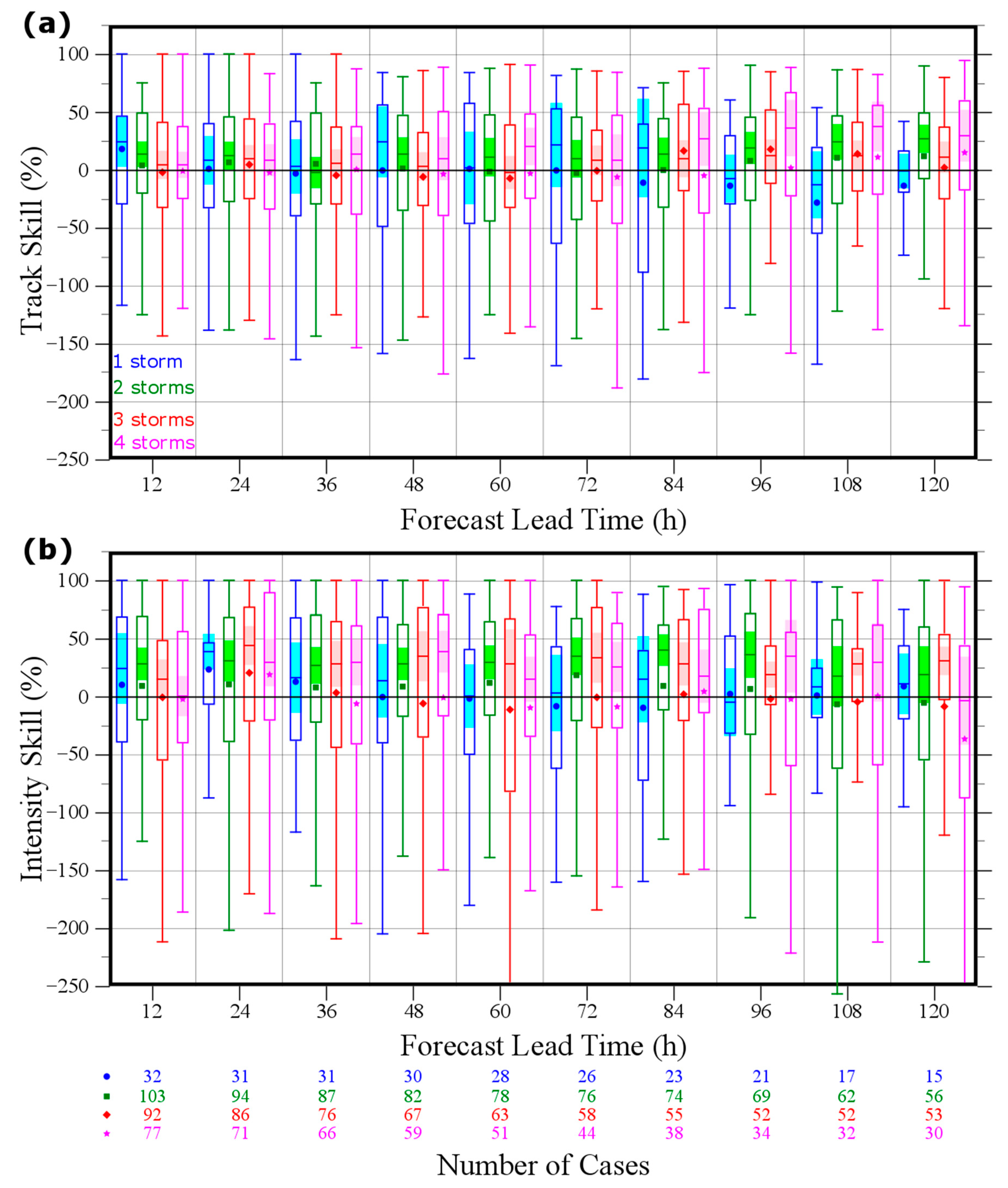
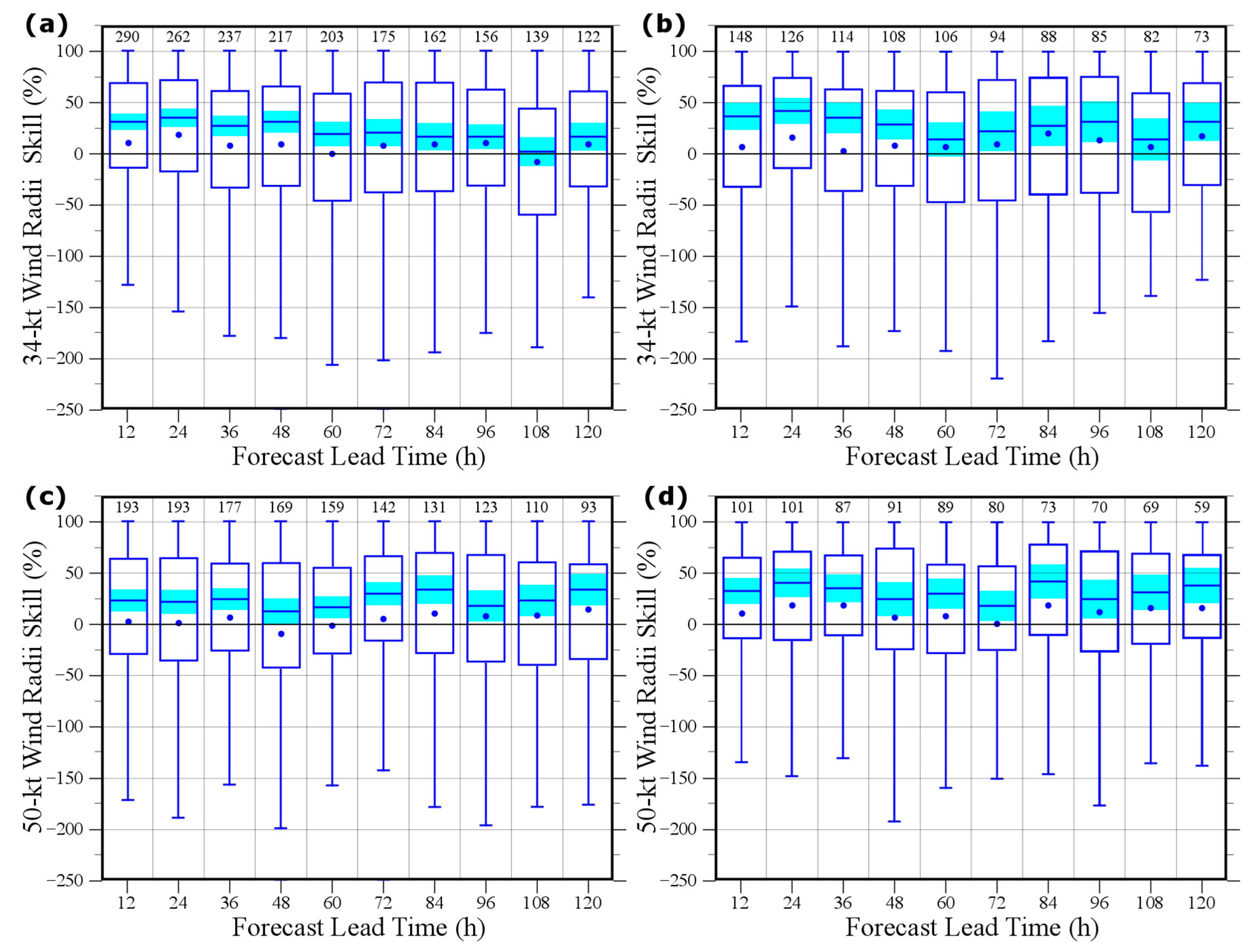
3. Forecast Verification

With the upgrade of both HWRF and HWRF-B to their respective 2020 versions, retrospective forecasts were produced and evaluated for priority TCs in the North Atlantic and eastern North Pacific basins from 2017–2019. TCs were prioritized based on discussions with NHC, resulting in 404 verifiable forecasts in the North Atlantic and 291 in the eastern North Pacific. The purpose of this verification is to determine if the multi-storm coupling scheme was implemented correctly with reasonable results by comparing HWRF-B forecasts with those from the operational HWRF, one of the best dynamical TC forecast models in recent years (21). In Figure 2, Figure 3, Figure 4 and Figure 5, track, intensity (i.e., maximum 10 m wind), and structure (i.e., 10 m wind radii) forecasts for HWRF-B and HWRF were verified in the North Atlantic and eastern North Pacific basins by comparing with the NHC best track [60]. Verifications followed NHC rules, which state that a forecast is verified only if the storm is classified as a TC at the initialization time and at the forecast time.

Relative forecast skill scores for HWRF-B were evaluated to concisely compare forecasts from HWRF-B with those from HWRF. Forecast skill scores for HWRF-B were computed by the following equation:

$$\mathrm{Skill}\mathrm{Score}=100·\left(1-\frac{B}{\overline{H}}\right),$$

(1)

where B is the absolute error from HWRF-B and $\overline{H}$ is the mean absolute error from HWRF used as a reference. Forecast skill scores may range from negative infinity (i.e., $\overline{H}$ = 0) to 100 (i.e., B = 0). Consequently, the distribution of skill scores can be skewed toward negative values by outliers. It is nonetheless valuable to know if forecasts are skillful at least 50% of the time, and, for this reason, the median and its statistical significance interval were critical to the evaluation. While outliers with large errors should be evaluated to help improve HWRF-B, it is important to remember that skill scores of this nature can result from very small HWRF errors ($\overline{H}\approx 0$ in Equation (1)).

Median skill scores for HWRF-B were statistically different from zero (i.e., represented forecast improvements over operational HWRF) at the 95% confidence level for TC track and intensity forecasts at all lead times in both the North Atlantic and eastern North Pacific, except for North Atlantic track skill at 36 h and eastern North Pacific track skill at 108 and 120 h (Figure 2). Median intensity skill scores in the North Atlantic were greater than 25% at every forecast lead time (Figure 2b). In general, median skill scores for intensity were higher in both basins than those for track. HWRF-B skill scores for North Atlantic TC track forecasts were higher at longer lead times (Figure 2a), consistent with Alaka et al. [24]. Mean skill scores were between −15% and 15% in both the North Atlantic and eastern North Pacific basins. Only 24 h mean intensity forecast skill in the North Atlantic was statistically significant at the 95% confidence level (not shown). In the North Atlantic, median and mean skill scores for track forecasts increased at longer lead times.

HWRF-B forecast skill scores were stratified by the number of storms at the forecast initialization time to evaluate the impact of HWRF-B’s multiple moving nests (Figure 3). Stratifying at the forecast initialization time is important for two main reasons: (1) the high-resolution moving nests in HWRF-B are only assigned at the beginning of the forecast, i.e., nests will not spawn for a TC that develops mid-forecast; and (2) a forecaster only knows how many storms are active when the forecast is made and does not know how many storms will be active at any time in the future. Median skill scores for TC track forecasts with multiple storms were noticeably greater for HWRF-B than HWRF at longer lead times (i.e., ≥96 h), suggesting that the improvement to median and mean skill scores is related to TCs that coexisted with other storms (compare Figure 3a with Figure 2a). Conversely, forecasts that were initialized with only one TC had near zero or negative mean and median relative skill scores at 96 h and later. Median skill scores for TC intensity forecasts were also higher for multiple storms, especially at 48–108 h lead times (Figure 3b). Forecasts initialized with only one TC had near-zero or negative mean and median skill scores over the same set of lead times. In general, the distribution of intensity skill scores from HWRF-B included a few skill scores <−150%, indicative of more volatility in intensity forecasts than track forecasts.

HWRF-B TC structure forecasts were also evaluated by comparing the radii of gale-force (34 kt) winds and storm-force (50 kt) winds with those from HWRF. At most forecast lead times, the median and mean skill scores for 34 and 50 kt wind radii errors were greater than zero for the full sample (Figure 4a,c). In fact, every median skill score was statistically greater than zero with 95% confidence except for 34 kt wind radii at 108 h lead times. Multiple moving nests positively contributed to storm size forecasts as well, with a combined sample of forecasts with either two or three storms at the model initialization time showing an increase in median and mean skill scores at most lead times, especially those later in the forecast (Figure 4b,d). The two-way feedback of the high-resolution moving nests with the outermost domain in HWRF-B allows concurrent storms to communicate with one another. As a result, this may lead to a more realistic atmospheric environment in a majority of forecasts, which previous studies have shown is critical for storm size predictions [61].

SST and its evolution have been shown to be important for TC intensity change [62]. With the implementation of the multi-storm coupler in HWRF-B, the distribution of HWRF-B intensity change is evaluated and compared with observations (Figure 5). HWRF-B 6 h intensity change magnitudes are generally too large when compared with the best track. This is reflected by HWRF-B having a larger standard deviation for intensity change than the best track by −1.5 kt / 6 h. Despite different shapes for each distribution, intensity change is normally distributed for both HWRF-B and the best track. Encouragingly, the interquartile range is nearly identical (−5 to 3 kt for HWRF-B versus −5 to 5 kt for the best track). Furthermore, the 95th and 5th percentiles of HWRF-B and best track distributions are 12 kt vs. 10 kt and −12 kt vs. −10 kt, respectively. It should be noted that 2 kt differences are within the noise of the best track [63]. The distribution of HWRF intensity change (not shown) was quite similar to that for HWRF-B.

4. Forecast Case Studies

Five HWRF-B forecasts from 2017–2019, for both the North Atlantic and eastern North Pacific, are evaluated to highlight the SST response that can be captured when several TCs interact with the ocean at high-resolution (

Table 1. Forecast initialization times used for HWRF-B case studies, showing corresponding active TCs with high-resolution nests coupled to MPIPOM-TC by the new coupling scheme.

Forecast Initialization Time	Storms with Nests
1800 UTC 18 September 2019	Kiko (EP132019), Lorena (EP152019), Mario (EP142019), Humberto (AL092019), Jerry (AL102019)
0600 UTC 12 September 2018	Florence (AL062018), Helene (AL082018), Isaac (AL092018), Olivia (EP172018), Paul (EP182018)
1200 UTC 31 August 2019	Dorian (AL052019), pre-Juliette (EP112019)
1200 UTC 03 September 2017	Irma (AL112017)
0600 UTC 15 September 2019	Kiko (EP132019), Humberto (AL092019)

). For comparison, a Level 4 optimally interpolated SST product combining microwave and infrared satellite radiances from Remote Sensing Systems (REMSS MWIR SST) [64] is shown for each forecast hour analyzed below. The SST response for the entire model domain and specific storms is also provided in one case to showcase the technology, the large ocean and outermost atmospheric domains, and the multi-storm forecasting capability.

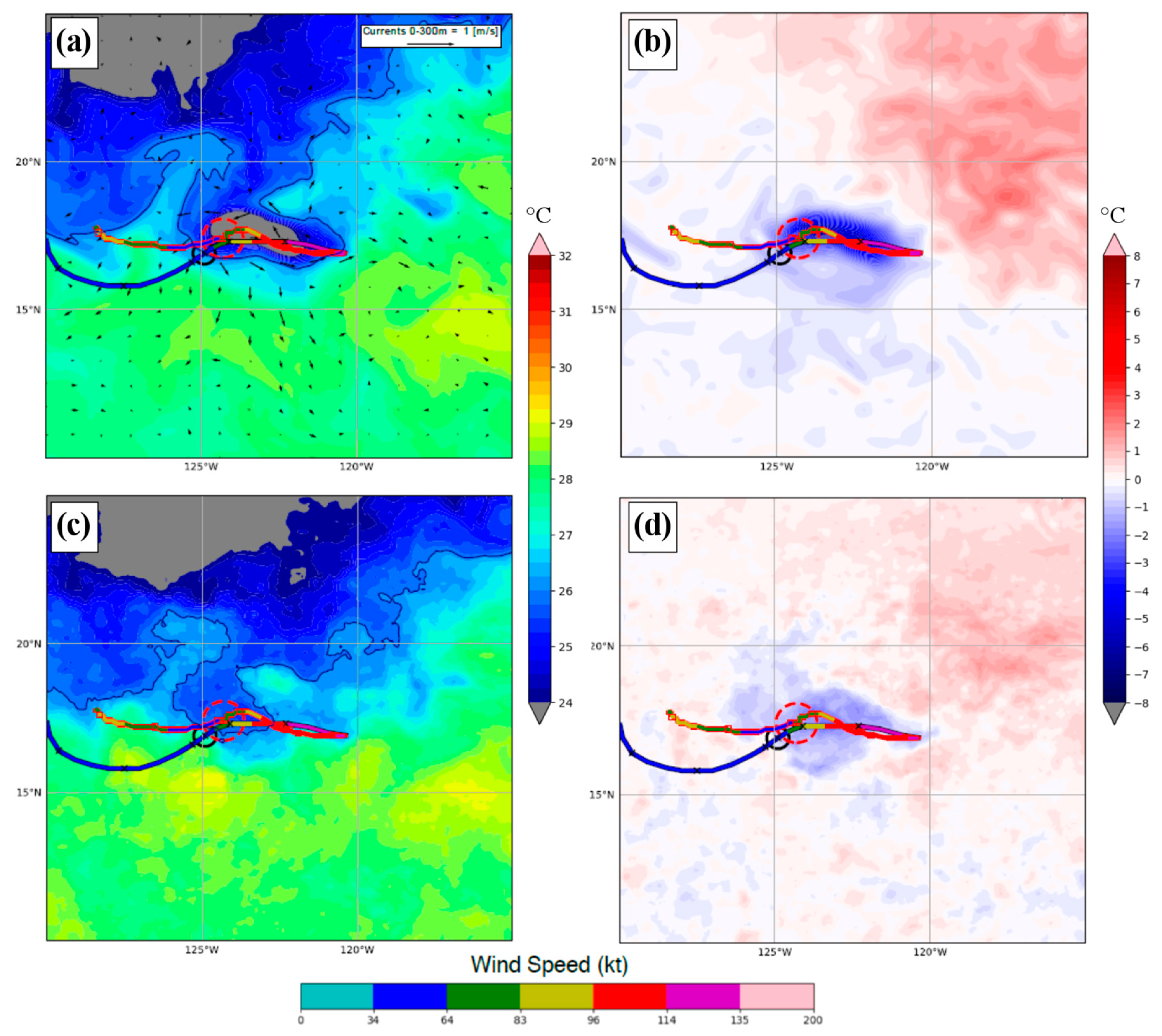
4.1. 1800. UTC 18 September 2019 (Mario EP142019)

For the HWRF-B forecast that was initialized at 1800 UTC 18 September 2019, five active TCs were simulated simultaneously at high resolution: Tropical Storm Kiko (EP132019), Tropical Storm Mario (EP142019), and Tropical Storm Lorena (EP152019) in the eastern North Pacific basin, and Hurricane Humberto (AL092019) and Tropical Storm Jerry (AL102019) in the North Atlantic basin. This forecast cycle highlighted the capability of the multi-storm coupling scheme to produce an efficient and realistic atmosphere/ocean exchange for several storms at high resolution.

The effect of these five coupled storms is readily observed in the MPIPOM-TC domain (Figure 6). The SST is shown for a 72 h forecast from HWRF-B and the corresponding MWIR data (Figure 6a,b). The tracks of individual TCs are shown, highlighting the SST cooling in both the model and observations. SST cooling is shown here and throughout, calculated relative to the initial forecast hour of the cycle (Figure 6c,d). The cold wake of Humberto in the model output shows its interaction with the Recirculation region and northern extension of the Gulf Stream, a major ocean current. In the eastern North Pacific, large areas of SST cooling >4 °C were predicted associated with Lorena and Mario, and, as will be seen below, this corresponded reasonably well with observed SST. There was also significant cooling associated with Kiko and Jerry at the forecast hour shown. As discussed below, the effect of 2–6 °C of cooling by Kiko may have contributed significantly to its forecast intensity.

The HWRF-B track and intensity forecast for Mario was particularly good, including an accurate simulation of slow movement northward as the TC interacted with Tropical Storm Lorena to its north. As a result, SST cooled by 2–7 °C near 16° N and 111° W with a minimum SST less than 24 °C (Figure 7a,b). The model forecast corresponded to a reasonably similar pattern of 2–4 °C cooling in the satellite observations, although the minimum observed SST was not as cold as the forecast (Figure 7c,d). The modeled ocean response was missing more cooling along the TC track to the north, which is likely the result of a slow-down of the simulated TC later in the forecast (black solid vs. red dashed and “x” in Figure 7).

Furthermore, widespread SST cooling was also evident near the track (not outlined) of Lorena near the southern tip of Baja California (see upper right of Figure 7b,d). The interaction between Mario and Lorena likely slowed the forward progress of both TCs, allowing for significant interaction with the ocean that was well-captured at high-resolution. Furthermore, the results in Figure 7 suggest that storm–storm interaction may have been observable in the ocean response to the two storms as well, albeit detailed evaluation of this possibility is beyond the scope of the present paper. It should be noted that SST cooling near coastlines, as was the case for Lorena, may be difficult to evaluate using remote sensing products, for reasons outlined in the Dorian case study (see Section 4.3). The significant cooling forecast along the shelf in the vicinity of Lorena, we surmise, is likely a result of the dynamical impact on the ocean by Mario.

4.2. 0600. UTC 12 September 2018 (Florence AL062018)

For the HWRF-B forecast that was initialized at 0600 UTC 12 September 2018, five active storms were simulated simultaneously at high-resolution: Hurricane Florence (AL062018), Hurricane Helene (AL082018), and Tropical Storm Isaac (AL092018) in the North Atlantic, plus Tropical Storm Olivia (EP172018) and Tropical Storm Paul (EP182018) in the eastern North Pacific. Florence, then a major hurricane, was on its final approach to landfall in North Carolina. In addition to being a very strong TC, Florence slowed down considerably as it approached land, increasing the importance of ocean coupling. Florence also coexisted with several additional TCs, making it a useful case for evaluating how multiple TCs interact with the same ocean model.

Florence’s track approaching landfall represents an interesting situation for a coupled air–sea TC model like HWRF-B. The TC first traversed the deeper waters of the western North Atlantic for a period of several days. It then crossed the axis of the Gulf Stream, a western boundary current and a deep, warm leg of the global meridional overturning circulation, just 18 h before its landfall. Furthermore, the continental shelf off the coast of North Carolina that was crossed by the TC, is narrow relative to the shelf that lies to its north and south along the coast. The opportunity to interact with both the deeper North Atlantic, the Gulf Stream, and, in short order, a narrow shelf—three very distinct oceanographic environments—represents a useful case study for a coupled model.

Florence created a long wake of SSTs that had cooled by 3–4 °C (Figure 8). This wake began near 29° N and 70° W and extended to the northwest toward the North Carolina coast, persistently to the right of the storm track. The observed SST cooling over open water (Figure 8c,d) was consistent with the MPIPOM-TC result (Figure 8a,b), suggesting that the ocean dynamics of the coupled system there responded well to the complex forcing of a strong, relatively slow-moving TC. The importance of coupling the nested domain to the ocean in this case was verified using an additional model run for the same initialization time, with the nest for Florence removed (not shown); the result shows significantly less SST cooling of only 1–3 °C, particularly in the region of the Gulf Stream and the shelf. On the other hand, a forecast cycle for this same time where ocean coupling was turned off (not shown) makes clear the value of the ocean coupling: this uncoupled forecast showed significantly greater maximum 10 m winds at most lead times, and a much greater intensity error, with maximum winds of 125 kt at 36 h as compared with 90–95 kt in the coupled forecast and best track.

Near landfall, the cold wake can be seen to propagate along the continental shelf of the eastern United States (Figure 8a,b) in the model forecast. As mentioned previously, model results near the coast may be difficult to evaluate using remote sensing products (see Dorian case study below). A detailed examination of this result in Florence is beyond the scope of the present paper; however, it appears as though this feature may be consistent with the joint effects of baroclinicity and relief and propagation of coastal vortical waves along the shelf [65].

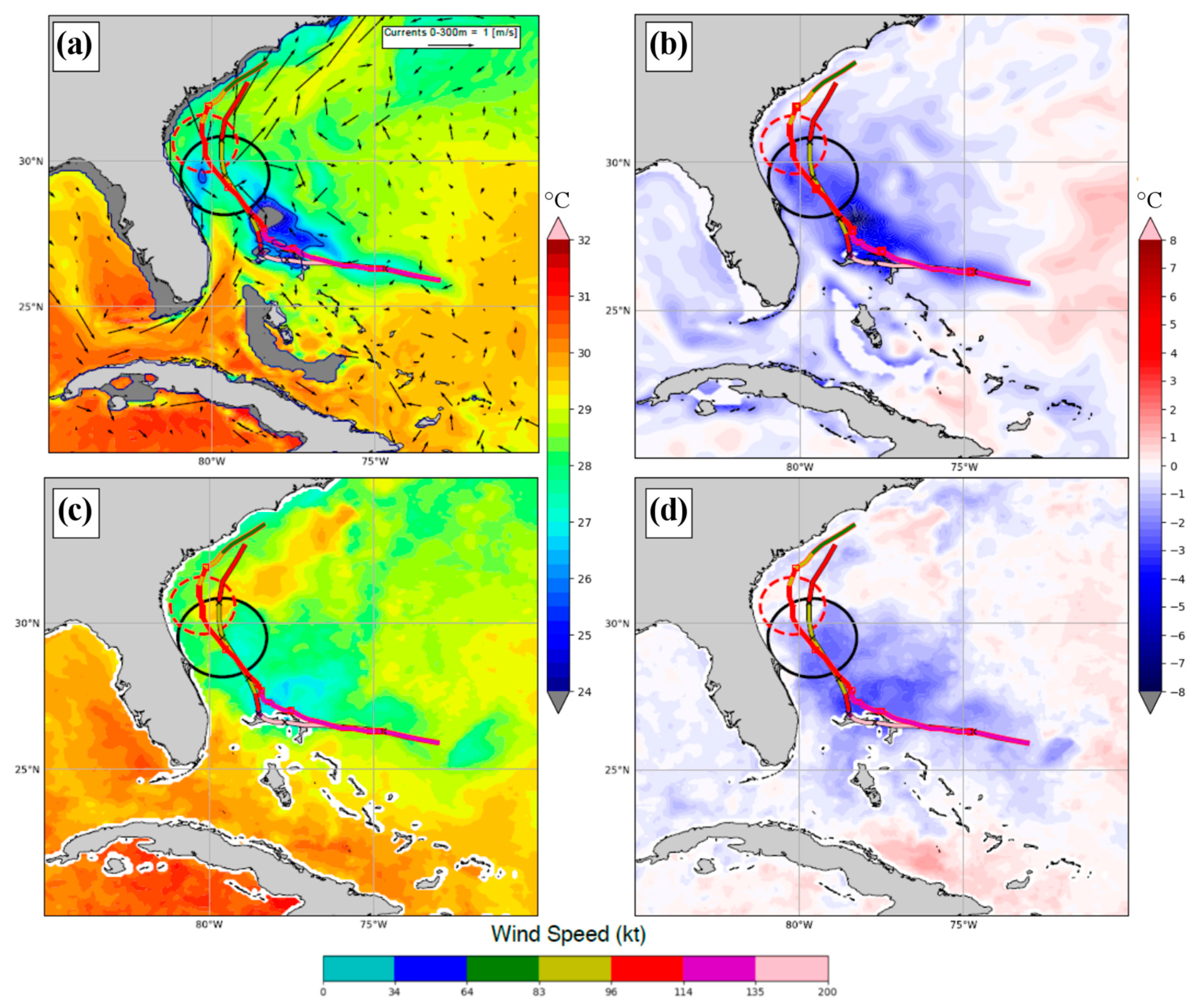
4.3. 1200. UTC 31 August 2019 (Dorian AL052019)

For the HWRF-B forecast that was initialized at 1200 UTC 31 August 2019, two active storms were simulated simultaneously at high-resolution: Hurricane Dorian (AL052019) in the North Atlantic and an invest that later developed into Hurricane Juliette (EP112019) in the eastern North Pacific. This forecast cycle was especially interesting because Hurricane Dorian stalled over very shallow waters in the northern Bahamas. Hurricane Dorian was also the strongest TC in the North Atlantic basin in 2019. Its absence of motion makes Dorian an excellent case with which to study HWRF-B ocean coupling.

During this forecast cycle, significant SST cooling of up to 8 °C and a large area of cooling of 4–5 °C near the northern Bahamas (Figure 9a,b) were generated in the coupled ocean model output. HWRF-B did not quite capture the stall of Dorian over the northern Bahamas, and, as a result, it was faster than observations, with an along-track error at the end of the cycle of over 150 km. The importance of coupling to the intensity forecast was verified with an uncoupled run of this same cycle, similar to that for Florence (above): that uncoupled run (not shown) maintained a maximum 10 m wind of over 130 kt from 63 to 84 h lead times, as compared with maximum winds of less than 110 kt in the coupled forecast.

Circulation patterns in the upper layer of the modeled ocean (black arrows, Figure 9a) suggest that interaction between the ocean and insular shelf and coastline of the Bahamas played a role in the evolution of temperature structure as well and potentially affected the forecast. The MWIR SST cooling apparent in the satellite observations of 1–4 °C was significantly less than that predicted; however, in this case, limitations of the MWIR satellite product may help explain this difference (Figure 9c,d). Land adjacency effects within 50 km of each of the Bahamas islands limited satellite SST coverage there largely to infrared radiances; such radiances are particularly vulnerable to contamination/filtering due to cloud cover, which was naturally prominent throughout Dorian’s passage. Such limitations in satellite data, by the way, may also have affected the RTOFS outputs used to initialize MPIPOM-TC; however, the approach of allowing a two-day, unforced spin up of MPIPOM-TC from initialization to first coupled forecast hour may have helped to remove such near-shore artifacts from this forecast.

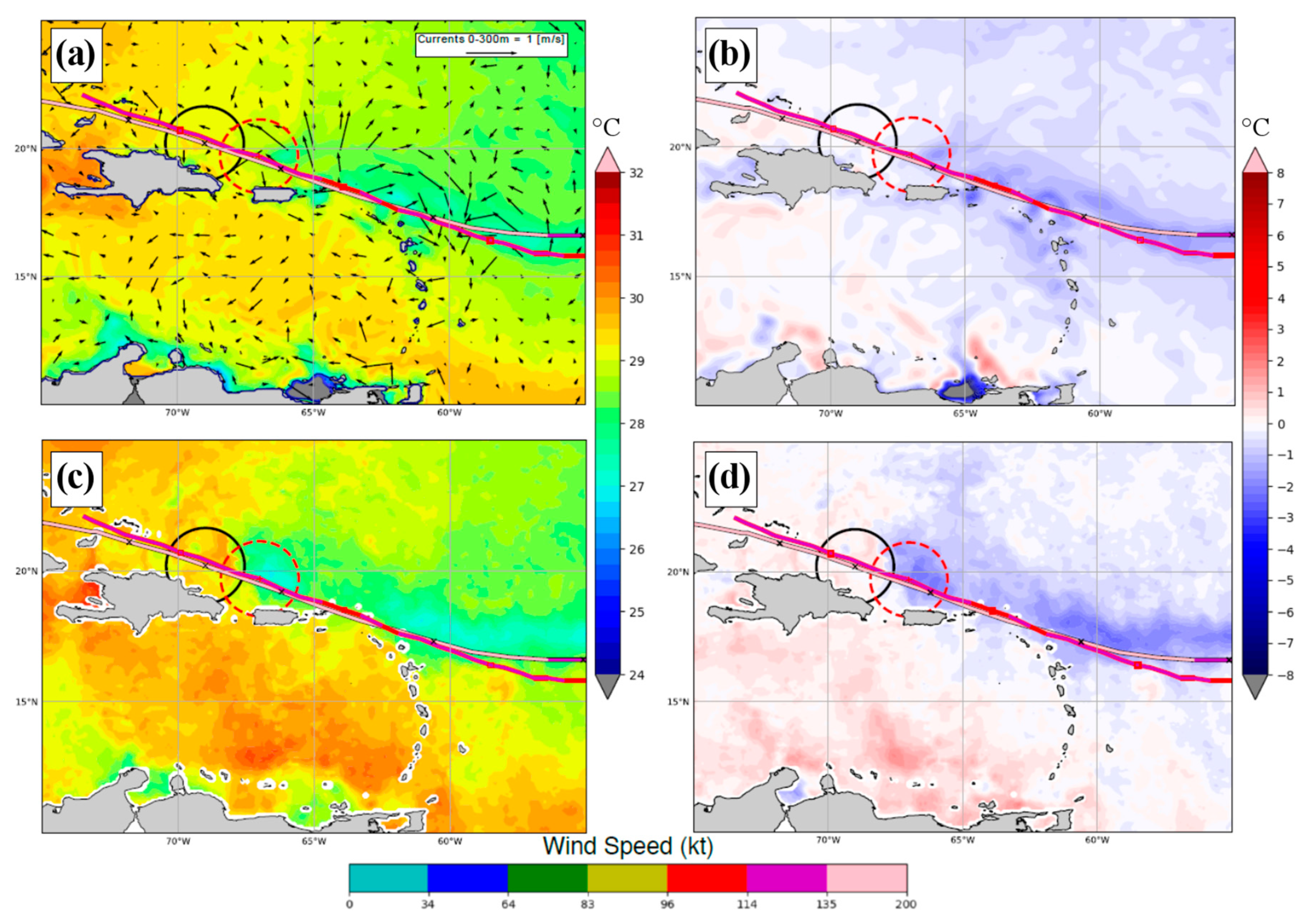
4.4. 1200. UTC 03 September 2017 (Irma AL112017)

For the HWRF-B forecast that was initialized at 1200 UTC 03 September 2017, Hurricane Irma (AL112017) was the only active storm in the North Atlantic simulated at high-resolution. Hurricane Irma was a major hurricane that would ultimately make landfall in Florida. Cooling of about 1–2 °C associated with Irma was forecast along its track with SST dropping to ~27 °C (Figure 10a,b). The magnitude of the cold wake observed in satellite SST was somewhat higher, being as great as 4 °C at certain points resulting in SST near 26 °C (Figure 10c,d). While the forward speed of Irma during the forecast period was somewhat less than best track, MPIPOM-TC may have missed the magnitude of cooling because the predicted intensity of the model storm was weaker than observations at several lead times. However, the lack of SST cooling in the model may also have been related to the depth of the 26 °C isotherm in the waters over which it passed. In general, initialization and evolution of mixed layer depth is critical in coupled TC modeling systems.

Features of the modeled upper ocean (<300 m) circulation match closely with some of the modeled SST cooling patterns in Figure 10a,b. This suggests that the dynamics of interaction between the storm and upper ocean are well captured by the coupled system. The effects of this interaction on the intensity of the TC are the subject of a current study with the HWRF-B system.

4.5. 0600. UTC 15 September 2019 (Kiko EP132019)

For the HWRF-B forecast that was initialized at 0600 UTC 15 September 2019, two active storms were simulated simultaneously at high-resolution: Tropical Storm Humberto (09L) in the North Atlantic and Hurricane Kiko (13E) in the eastern North Pacific. The track of Kiko lay near an SST front in the eastern North Pacific and an area of relatively low heat potential that was well captured by the coupled ocean–atmosphere model (Figure 11a). Widespread SST cooling of 2–6 °C was observed in the model forecast to the right of Kiko’s track (Figure 11b). A similar pattern of SST and SST cooling from 2–3 °C was seen in the satellite observations (Figure 11c,d). The difference between modeled and best track translation speeds likely resulted in greater cooling in the model than was observed by satellite. This region of cooling corresponded to weakening the intensity of Kiko. This is particularly significant because the initial SST front lay well to the north of Kiko’s track, highlighting the likely effect of the SST cooling from the coupled ocean response on the storm’s modeled evolution. The importance of this modeled cooling to the intensity forecast was verified with a separate run of the same forecast cycle where ocean coupling was turned off. Similar to the cases of Florence and Dorian above, forecast maximum 10 m winds for Kiko were 30–35 kt greater than best track in the uncoupled case, as compared with 15–20 kt intensity errors for the coupled run.

5. Conclusions

The motivation of this paper is to report the results from an advanced multi-storm coupled hydrodynamical modeling system, called HWRF-B. HWRF-B was developed to improve TC forecasts by allowing multiple TCs to interact directly, with high-resolution storm-following nests in a single large regional domain that spans NHC’s entire area of responsibility. A new and efficient multi-storm coupling scheme was implemented in the 2020 version of HWRF-B, which was based on the single-storm coupling scheme currently in the operational HWRF. With the addition of the new coupling scheme, HWRF-B has become a state-of-the-art coupled modeling system capable of simulating the interaction of several TCs with the ocean at high resolution. The coupling scheme is available for implementation in any atmosphere/ocean modeling system, including those with storm-following nests.

Overall, the present paper demonstrates that the new coupling scheme was implemented correctly in HWRF-B by evaluating retrospective TC forecasts for NHC-prioritized TCs over a three-year period and by analyzing the SST response to six different case study TCs in particular. Median track, intensity, and structure forecasts from HWRF-B were significantly better than those from the storm-centric HWRF. Mean skill scores of HWRF-B relative to HWRF were closer to zero, in part due to the impact of outlier forecasts with large, negative skill scores. In addition, the distribution of 6 h intensity-change forecasts from HWRF-B across these priority TCs was quite similar to that from the NHC best track. Forecast skill was found to be a function of the number of storms present at the model initialization time, with skill scores generally improving with more storms. This result provides evidence that the multi-storm modeling approach can improve TC forecast skill. The multi-storm configuration in HWRF-B could be applied to global models to produce multiple high-resolution forecasts in less time and at a lower computational cost. HWRF-B is currently being used to better understand multi-storm interactions of all types, including binary interactions (e.g., Mario and Lorena, see Section 4.1), intermediate interactions (e.g., Florence and Isaac, see Section 4.2), and long-range interactions between storms in difference ocean basins (e.g., Humberto in the North Atlantic and Kiko in the eastern North Pacific, see Section 4.1 and Section 4.5).

A detailed comparison of model results to observation is beyond the scope of this paper. However, the examination of five case studies (including details on six TCs) shows that key features of upper ocean dynamics under TC forcing, as revealed by SST evolution, are substantially reproduced by the coupled modeling system. The results for these case studies also suggest, as discussed above, that the coupling between ocean and atmosphere through the newly developed multi-storm coupling scheme captures essential ocean–atmosphere interactions that are important for skillful TC intensity forecasts. These cases show the coupled system at work, modeling air–sea interaction under a broad range of TC intensities and with a broad range of storm translation speeds, representative of many observed storms in the chosen domain. The range of case studies chosen includes forecasts from 2017–2019 in both the Atlantic and eastern Pacific basins, showing the ocean response to TCs under a range of regional and basin-wide ocean near-surface conditions found during those three years. It is important to note that all but one of the cases (1200 UTC 03 September 2017 for Irma) show some type of multi-storm interaction (i.e., binary, intermediate, remote). The Irma case was included to demonstrate that the multi-storm coupling scheme can be applied to a single-storm forecast as well, meaning this new technology could be seamlessly applied to the single-storm operational HWRF and other storm-centric models.

This and other recent work [23] has shown the viability of using a multi-storm approach to TC forecasting for both research and operations. HWRF-B has provided a useful blueprint on multiple moving nests and how they interact with an ocean model, which will guide future developments at NOAA. To improve and extend TC forecasts is a key goal of NOAA’s Unified Forecast System (UFS) [66,67,68]. Within UFS, the Hurricane Analysis and Forecast System (HAFS) [26,69,70] is being developed with a multi-storm approach, with HWRF-B providing a unique baseline for simulating multiple TCs at high resolution. This version of HWRF-B will also be useful for the continued development of coupled atmosphere/ocean data assimilation, which will be critical in improving analyses and subsequent forecasts in HAFS. In future work, a more comprehensive assessment of multi-storm interactions will be performed with HWRF-B to shed light on the dynamics and thermodynamics involved and, ultimately, to improve TC forecast guidance further. The case studies evaluated in this manuscript will be foundational to this future work. A necessary part of this assessment is an evaluation of air–sea interaction and underlying ocean vertical structure in TCs, which can be investigated thoroughly using the multi-storm atmosphere/ocean coupling scheme described in this study. To this end, multi-storm interactions in air–sea coupled HWRF-B forecasts are the subject of a detailed, ongoing evaluation by the authors.

References

1. Cione, J. The Relative Roles of the Ocean and Atmosphere as Revealed by Buoy Air–Sea Observations in Hurricanes. Mon. Weather Rev. 2015, 143, 904–913. [Google Scholar] [CrossRef]
2. Tuleya, R.E.; Kurihara, Y. A note on the sea surface temperature sensitivity of a numerical model of tropical storm genesis. Mon. Weather Rev. 1982, 110, 2063–2069. [Google Scholar] [CrossRef] [Green Version]
3. Emanuel, K.A. An Air-Sea Interaction Theory for Tropical Cyclones. Part I: Steady-State Maintenance. J. Atmos. Sci. 1986, 43, 585–605. [Google Scholar] [CrossRef]
4. Holland, G.J. Maximum potential intensity of tropical cyclones. J. Atmos. Sci. 1997, 54, 2519–2541. [Google Scholar] [CrossRef]
5. Black, P.G. Ocean Temperature Changes Induced by Tropical Cyclones. Ph.D. Thesis, The Pennsylvania State University, University Park, PA, USA, 1983. [Google Scholar]
6. Bender, M.A.; Ginis, I.; Kurihara, Y. Numerical simulations of tropical cyclone-ocean interaction with a high resolution coupled model. J. Geophys. Res. 1993, 98, 23245–23263. [Google Scholar] [CrossRef]
7. Halliwell, G.R.; Gopalakrishnan, S.G.; Marks, F.D.; Willey, D. Idealized Study of Ocean Impacts on Tropical Cyclone Intensity Forecasts. Mon. Weather Rev. 2015, 143, 1142–1165. [Google Scholar] [CrossRef]
8. Price, J. Upper Ocean Response to a Hurricane. J. Phys. Oceanogr. 1981, 11, 153–175. [Google Scholar] [CrossRef] [Green Version]
9. Yablonsky, R.M.; Ginis, I. Limitation of one-dimensional ocean models for coupled hurricane–ocean model forecasts. Mon. Weather Rev. 2009, 137, 4410–4419. [Google Scholar] [CrossRef]
10. Jaimes, B.; Shay, L.K. Mixed layer cooling in mesoscale oceanic eddies during Hurricanes Katrina and Rita. Mon. Weather Rev. 2009, 137, 4188–4207. [Google Scholar] [CrossRef] [Green Version]
11. Yablonsky, R.M.; Ginis, I. Impact of a warm ocean eddy’s circulation on hurricane-induced sea surface cooling with implications for hurricane intensity. Mon. Weather Rev. 2013, 141, 997–1021. [Google Scholar] [CrossRef] [Green Version]
12. Bao, J.-W.; Wilczak, J.M.; Choi, J.-K.; Kantha, L.H. Numerical simulations of air-sea interaction under high wind conditions using a coupled model: A study of hurricane development. Mon. Weather Rev. 2000, 128, 2190–2210. [Google Scholar] [CrossRef]
13. Bender, M.A.; Ginis, I. Real-case simulations of hurricane–ocean interaction using a high-resolution coupled model: Effects on hurricane intensity. Mon. Weather Rev. 2000, 128, 917–946. [Google Scholar] [CrossRef]
14. Gopalakrishnan, S.G.; Marks, F.D.; Zhang, X.; Bao, J.-W.; Yeh, K.-S.; Atlas, R. The experimental HWRF system: A study on the influence of horizontal resolution on the structure and intensity changes in tropical cyclones using an idealized framework. Mon. Weather Rev. 2011, 139, 1762–1784. [Google Scholar] [CrossRef]
15. Gopalakrishnan, S.G.; Goldenberg, S.B.; Quirino, T.S.; Zhang, X.; Marks, F.D.; Yeh, K.-S.; Atlas, R.; Tallapragada, V. Toward improving high-resolution numerical hurricane forecasting: Influence of model horizontal grid resolution, initialization, and physics. Weather Forecast. 2012, 27, 647–666. [Google Scholar] [CrossRef]
16. Gopalakrishnan, S.G.; Marks, F.D.; Zhang, J.A.; Zhang, X.; Bao, J.-W.; Tallapragada, V. A study of the impacts of vertical diffusion on the structure and intensity of the tropical cyclones using the high resolution HWRF system. J. Atmos. Sci. 2013, 70, 524–541. [Google Scholar] [CrossRef]
17. Bao, J.-W.; Gopalakrishnan, S.G.; Michelson, S.A.; Marks, F.D.; Montgomery, M.T. Impact of physics representations in the HWRFX on simulated hurricane structure and pressure–wind relationships. Mon. Weather Rev. 2012, 140, 3278–3299. [Google Scholar] [CrossRef] [Green Version]
18. Tallapragada, V.; Kieu, C.; Kwon, Y.; Trahan, S.; Liu, Q.; Zhang, Z.; Kwon, I.-H. Evaluation of storm structure from the operational HWRF model during 2012 implementation. Mon. Weather Rev. 2014, 142, 4308–4325. [Google Scholar] [CrossRef]
19. Atlas, R.; Tallapragada, V.; Gopalakrishnan, S.G. Advances in tropical cyclone intensity forecasts. Mar. Technol. J. 2015, 49, 149–160. [Google Scholar] [CrossRef]
20. Mehra, A.; Tallapragada, V.; Zhang, Z.; Liu, B.; Zhu, L.; Wang, W.; Kim, H.-S. Advancing the State of the Art in Operational Tropical Cyclone Forecasting at NCEP. Trop. Cyclone Res. Rev. 2018, 7, 51–56. [Google Scholar] [CrossRef]
21. Cangialosi, J.P. 2019 Hurricane Season; National Hurricane Center Forecast Verification Report; National Hurricane Center: Miami, FL, USA, 2020; 75p. Available online: http://www.nhc.noaa.gov/verification/pdfs/Verification_2019.pdf (accessed on 25 April 2020).
22. Zhang, X.; Gopalakrishnan, S.G.; Trahan, S.; Quirino, T.S.; Liu, Q.; Zhang, Z.; Alaka, G.J.; Tallapragada, V. Representing multiple scales in the hurricane weather research and forecasting modeling system: Design of multiple sets of movable multilevel nesting and the basin-scale HWRF forecast application. Weather Forecast. 2016, 31, 2019–2034. [Google Scholar] [CrossRef]
23. Alaka, G.J.; Zhang, X.; Gopalakrishnan, S.G.; Goldenberg, S.B.; Marks, F.D. Performance of basin-scale HWRF tropical cyclone track forecasts. Weather Forecast. 2017, 32, 1253–1271. [Google Scholar] [CrossRef]
24. Alaka, G.J.; Zhang, X.; Gopalakrishnan, S.G.; Zhang, Z.; Marks, F.D.; Atlas, R. Track Uncertainty in High-Resolution HWRF Ensemble Forecasts of Hurricane Joaquin. Weather Forecast. 2019, 34, 1889–1908. [Google Scholar] [CrossRef]
25. Gall, R.; Franklin, J.; Marks, F.; Rappaport, E.N.; Toepfer, F. The Hurricane Forecast Improvement Project. Bull. Am. Meteorol. Soc. 2013, 94, 329–343. [Google Scholar] [CrossRef]
26. Gopalakrishnan, S.G.; Coauthors. 2019 HFIP R&D Activities Summary: Recent Results and Operational Implementation; NOAA HFIP Technical Report HFIP2020-1; NOAA: Silver Spring, MD, USA, 2020; 42p. Available online: http://www.hfip.org/documents/HFIP_AnnualReport_FY2019.pdf (accessed on 3 May 2020).
27. Janjic, Z.; Coauthors. User’s Guide for the NMM Core of the Weather Research and Forecast (WRF) Modeling System Version 4; NCAR Technical Note; NCAR: Boulder, CO, USA, 2018; 123p, Available online: https://dtcenter.org/HurrWRF/users/docs/scientific_documents/WRF-NMM_2018.pdf (accessed on 11 April 2020).
28. Rogers, E.; Black, T.; Ferrier, B.; Lin, Y.; Parrish, D.; DiMego, G. NCEP Meso Eta Analysis and Forecast System: Increase in resolution, new cloud microphysics, modified precipitation assimilation, modified 3DVAR analysis. NWS Tech. Proced. Bull. 2001, 488, 1–15. [Google Scholar]
29. Ferrier, B.S.; Jin, Y.; Lin, Y.; Black, T.; Rogers, E.; DiMego, G. Implementation of a new grid-scale cloud and precipitation scheme in the NCEP Eta model. In Proceedings of the 19th Conference on Weather Analysis and Forecasting/15th Conference on Numerical Weather Prediction, San Antonio, TX, USA, 15 August 2002; Available online: https://ams.confex.com/ams/SLS_WAF_NWP/techprogram/paper_47241.htm (accessed on 17 March 2020).
30. Arakawa, A.; Schubert, W.H. Interaction of a Cumulus Cloud Ensemble with the Large-Scale Environment, Part I. J. Atmos. Sci. 1974, 31, 674–701. [Google Scholar] [CrossRef] [Green Version]
31. Grell, G.J.A.J. Prognostic evaluation of assumptions used by cumulus parameterizations. Mon. Weather Rev. 1993, 121, 764–787. [Google Scholar] [CrossRef] [Green Version]
32. Pan, H.-L.; Wu, J. Implementing a Mass Flux Convection Parameterization Package for the NMC Medium-Range Forecast Model; NMC Office Note No. 409; NOAA: Silver Spring, MD, USA, 1995; 40p. Available online: https://repository.library.noaa.gov/view/noaa/11429 (accessed on 17 March 2020).
33. Kwon, Y.C.; Lord, S.; Lapenta, B.; Tallapragada, V.; Liu, Q.; Zhang, Z. Sensitivity of Air-Sea Exchange Coefficients (Cd and Ch) on Hurricane Intensity. In Proceedings of the 29th Conference on Hurricanes and Tropical Meteorology, American Meteorological Society, Tucson, AZ, USA, 13 May 2010; Available online: https://ams.confex.com/ams/29Hurricanes/webprogram/Paper167760.html (accessed on 15 March 2020).
34. Powell, M.D.; Vickery, P.J.; Reinhold, T.A. Reduced drag coefficient for high wind speeds in tropical cyclones. Nature 2003, 422, 279–283. [Google Scholar] [CrossRef]
35. Black, P.G.; D’Asaro, E.A.; Drennan, W.M.; French, J.R.; Sanford, T.B.; Terrill, E.J.; Niiler, P.P.; Walsh, E.J.; Zhang, J. Air-Sea Exchange in Hurricanes: Synthesis of Observations from the Coupled Boundary Layer Air-Sea Transfer Experiment. Bull. Am. Meteorol. Soc. 2007, 88, 357–374. [Google Scholar] [CrossRef] [Green Version]
36. Mahrt, L.; Ek, M. The influence of atmospheric stability on potential evaporation. J. Clim. Appl. Meteorol. 1984, 23, 222–234. [Google Scholar] [CrossRef] [Green Version]
37. Mahrt, L.; Pan, H.L. A two-layer model of soil hydrology. Bound. Layer Meteorol. 1984, 29, 1–20. [Google Scholar] [CrossRef]
38. Pan, H.-L.; Mahrt, L. Interaction between soil hydrology and boundary-layer development. Bound. Layer Meteorol. 1987, 38, 185–202. [Google Scholar] [CrossRef]
39. Chen, F.; Coauthors. Modeling of land-surface evaporation by four schemes and comparison with FIFE observations. J. Geophys. Res. 1996, 101, 7251–7268. [Google Scholar] [CrossRef] [Green Version]
40. Schaake, J.C.; Koren, V.I.; Duan, Q.Y.; Mitchell, K.; Chen, F. A simple water balance model (SWB) for estimating runoff at different spatial and temporal scales. J. Geophys. Res. 1996, 101, 7461–7475. [Google Scholar] [CrossRef]
41. Chen, F.; Dudhia, J.; Janjic, Z.; Baldwin, M. Coupling a land-surface model to the NCEP mesoscale Eta model. In Proceedings of the 13th Conference on Hydrology, Long Beach, CA, USA, 2–7 February 1997; pp. 99–100. [Google Scholar]
42. Koren, V.; Schaake, J.; Mitchell, K.; Duan, Q.-Y.; Chen, F. A parameterization of snowpack and frozen ground intended for NCEP weather and climate models. J. Geophys. Res. 1999, 104, 19569–19585. [Google Scholar] [CrossRef]
43. Ek, M.B.; Mitchell, K.E.; Lin, Y.; Rogers, E.; Grunmann, P.; Koren, V.; Gayno, G.; Tarpley, J.D. Implementation of Noah land surface model advancements in the National Centers for Environmental Pre- diction operational mesoscale Eta model. J. Geophys. Res. 2003, 108, 8851. [Google Scholar] [CrossRef]
44. Troen, I.; Mahrt, L. A simple model of the atmospheric boundary layer: Sensitivity to surface evaporation. Bound. Layer Meteorol. 1986, 37, 129–148. [Google Scholar] [CrossRef]
45. Hong, S.-Y.; Pan, H.-L. Nonlocal boundary layer vertical diffusion in a medium-range forecast model. Mon. Weather Rev. 1996, 124, 2322–2339. [Google Scholar] [CrossRef] [Green Version]
46. Han, J.; Witek, M.; Teixeira, J.; Sun, R.; Pan, H.-L.; Fletcher, J.K.; Bretherton, C.S. Implementation in the NCEP GFS of a Hybrid Eddy-Diffusivity Mass-Flux (EDMF) Boundary Layer Parameterization with Dissipative Heating and Modified Stable Boundary Layer Mixing. Weather Forecast. 2016, 31, 341–352. [Google Scholar] [CrossRef]
47. Mlawer, E.; Taubman, S.; Brown, P.; Iacono, M.; Clough, S. Radiative transfer for inhomogeneous atmosphere: RRMT, a validated corelated-k model for the longwave. J. Geophys. Res. 1997, 102, 16663–16682. [Google Scholar] [CrossRef] [Green Version]
48. Iacono, M.J.; Delamere, J.S.; Mlawer, E.J.; Shephard, M.W.; Clough, S.A.; Collins, W.D. Radiative forcing by long-lived greenhouse gases: Calculations with the AER radiative transfer models. J. Geophys. Res. 2008, 113, D13103. [Google Scholar] [CrossRef]
49. Biswas, M.K.; Carson, L.; Newman, K.; Stark, D.; Kalina, E.; Grell, E.; Frimel, J. Community HWRF Users’ Guide V4.0a; NCAR: Boulder, CO, USA, 2018; 162p, Available online: https://dtcenter.org/sites/default/files/community-code/hwrf/docs/users_guide/HWRF-UG-2018.pdf (accessed on 16 March 2020).
50. Liu, Q.; Surgi, N.; Lord, S.; Wu, W.-S.; Parrish, D.; Gopalakrishnan, S.G.; Waldrop, J.; Gamache, J. Hurricane Initialization in HWRF Model. In Proceedings of the 27th Conference on Hurricanes and Tropical Meteorology, American Meteorological Society, Monterey, CA, USA, 26 April 2006; Available online: https://ams.confex.com/ams/pdfpapers/108496.pdf (accessed on 17 March 2020).
51. Wu, W.-S.; Purser, R.J.; Parrish, D.F. Three-dimensional variational analysis with spatially inhomogeneous covariances. Mon. Weather Rev. 2002, 130, 2905–2916. [Google Scholar] [CrossRef] [Green Version]
52. Tong, M.; Coauthors. Impact of Assimilating Aircraft Reconnaissance Observations on Tropical Cyclone Initialization and Prediction Using Operational HWRF and GSI Ensemble–Variational Hybrid Data Assimilation. Mon. Weather Rev. 2018, 146, 4155–4177. [Google Scholar] [CrossRef]
53. Lu, X.; Wang, X.; Li, Y.; Tong, M.; Ma, X. GSI-based ensemble-variational hybrid data assimilation for HWRF for hurricane initialization and prediction: Impact of various error covariances for airborne radar observation assimilation. Q. J. R. Meteorol. Soc. 2017, 143, 223–239. [Google Scholar] [CrossRef]
54. Lu, X.; Wang, X.; Tong, M.; Tallapragada, V. GSI-Based, Continuously Cycled, Dual-Resolution Hybrid Ensemble–Variational Data Assimilation System for HWRF: System Description and Experiments with Edouard (2014). Mon. Weather Rev. 2017, 145, 4877–4898. [Google Scholar] [CrossRef]
55. Blumberg, A.F.; Mellor, G.L. A description of a three-dimensional coastal ocean circulation model. In Three-Dimensional Coastal Ocean Models, 4th ed.; Heaps, N.S., Ed.; American Geophysical Union: Washington, DC, USA, 1987; Volume 4, pp. 1–16. [Google Scholar] [CrossRef]
56. Yablonsky, R.M.; Ginis, I.; Thomas, B. Ocean modelling with flexible initialization for improved coupled tropical cyclone-ocean model prediction. Environ. Model. Softw. 2015, 67, 26–30. [Google Scholar] [CrossRef]
57. Mellor, G.L. Users Guide for a Three-Dimensional, Primitive Equation, Numerical Ocean Model (June 2004 Version); Program in Atmospheric and Oceanic Sciences; Princeton University: Princeton, NJ, USA, 2004; 56p. [Google Scholar]
58. Mehra, A.; Rivin, I. A real time ocean forecast system for the North Atlantic Ocean. Terr. Atmos. Ocean. Sci. 2010, 21, 211–228. [Google Scholar] [CrossRef] [Green Version]
59. Bender, M.A.; Ginis, I.; Tuleya, R.; Thomas, B.; Marchok, T. The operational GFDL coupled hurricane–ocean prediction system and a summary of its performance. Mon. Weather Rev. 2007, 135, 3965–3989. [Google Scholar] [CrossRef]
60. Rappaport, E.N.; Coauthors. Advances and challenges at the National Hurricane Center. Weather Forecast. 2009, 24, 395–419. [Google Scholar] [CrossRef] [Green Version]
61. Hill, K.A.; Lackmann, G.M. Influence of Environmental Humidity on Tropical Cyclone Size. Mon. Weather Rev. 2009, 137, 3294–3315. [Google Scholar] [CrossRef]
62. Chan, J.C.L.; Duan, Y.; Shay, L.K. Tropical Cyclone Intensity Change from a Simple Ocean–Atmosphere Coupled Model. J. Atmos. Sci. 2001, 58, 154–172. [Google Scholar] [CrossRef]
63. Torn, R.D.; Snyder, C. Uncertainty of Tropical Cyclone Best-Track Information. Weather Forecast. 2012, 27, 715–729. [Google Scholar] [CrossRef]
64. Reynolds, R.W.; Gentemann, C.L.; Wentz, F. Impact of TRMM SSTs on a climate-scale SST analysis. J. Clim. 2004, 17, 2938–2952. [Google Scholar] [CrossRef]
65. Chen, K.; He, R.; Powell, B.S.; Gawarkiewicz, G.G.; Moore, A.M.; Arango, H.G. Data assimilative modeling investigation of Gulf Stream Warm Core Ring interaction with continental shelf and slope circulation. J. Geophys. Res. Ocean. 2014, 119, 5968–5991. [Google Scholar] [CrossRef] [Green Version]
66. Auligne, T.; Coauthors. Unified Modeling System Architecture Overview. NOAA UFS Technical Report; NOAA: Silver Spring, MD, USA, 2016; 10p. Available online: https://drive.google.com/file/d/1LV0E0F1M6xKAQ3iQ-UG8llpVhH2hUE7F/view (accessed on 18 May 2020).
67. Rood, R.B.; Coauthors. Organizing Research to Operations; NOAA UFS Technical Report; NOAA: Silver Spring, MD, USA, 2018; 36p. Available online: http://ufs-dev.rap.ucar.edu/docs/Repository/20181130_Organizing_Research_to_Operations_Transition.pdf (accessed on 18 May 2020).
68. Tallapragada, V. Proposed Implementation of Global Ensemble Forecast System, Version 12.0; NOAA UFS Technical Report; NOAA: Silver Spring, MD, USA, 2020. Available online: http://ufs-dev.rap.ucar.edu/docs/Repository/20200302_Eval_Letter_GEFSv12.pdf.pdf (accessed on 18 May 2020).
69. Dong, J.; Liu, B.; Zhang, Z.; Wang, W.; Zhu, L.; Zhang, C.; Wu, K.; Hazelton, A.; Zhang, X.; Mehra, A.; et al. Hurricane Analysis and Forecast System (HAFS) Stand-Alone Regional Model (SAR) 2019 Atlantic Hurricane Season Real-Time Forecasts. In Proceedings of the 2020 Annual Meeting, American Meteorological Society, Boston, MA, USA, 15 January 2020; Available online: https://ams.confex.com/ams/2020Annual/webprogram/Paper368586.html (accessed on 19 May 2020).
70. Hazelton, A.; Zhang, Z.; Dong, J.; Liu, B.; Wang, W.; Alaka, G.J.; Zhang, X.; Zhang, C.; Zhu, L.; Wu, K.; et al. The Global-Nested Hurricane Analysis and Forecast System (HAFS): Results from the 2019 Atlantic Hurricane Season. In Proceedings of the 2020 Annual Meeting, American Meteorological Society, Boston, MA, USA, 15 January 2020; Available online: https://ams.confex.com/ams/2020Annual/webprogram/Paper367614.html (accessed on 19 May 2020).
Figure 1. (a) Mean sea-level pressure (shaded) within the outermost domain of the atmosphere model, the Basin-scale Hurricane Weather Research ad Forecasting (HWRF-B) model. The domain of the ocean model, the Message Passing Interface Princeton Ocean Model for Tropical Cyclones (MPIPOM-TC), is outlined with a dashed black line. Moving nests (two per storm) are shown for four storms. (b) The schematic shows the model tree for the entire HWRF-B modeling system, specifically: HWRF-B (red; the atmosphere model), MPIPOM-TC (blue; the ocean model), the multi-storm coupling scheme (yellow), and initial/lateral boundary conditions (green), including the Global Forecast System (GFS) and the Global Real-Time Ocean Forecast System (RTOFS). Arrows show the flow of data: green arrows represent initial/lateral boundary conditions, red arrows represent internal data flow within HWRF-B, and black arrows represent data transferred by the coupling scheme. The schematic shows a forecast with two storms: tropical cyclone 1 (TC1) and tropical cyclone 2 (TC2).
Atmosphere 11 00869 g001
Figure 2. Box-and-whisker plots showing the distribution of HWRF-B forecast skill scores versus HWRF (Equation (1)) for 2017–2019 priority tropical cyclones (TCs) and 12–120 h forecast lead times in the (a,b) North Atlantic and (c,d) eastern North Pacific. Track forecast skill is shown in (a,c), and intensity forecast skill is shown in (b,d). The median is designated by a horizontal line within the box, and the sample mean is provided by a circle. The top (bottom) of the box represents the 75th (25th) percentile. The top whisker represents the smaller value of the maximum and the 75th percentile plus 150% of the interquartile range (IQR). The bottom whisker represents the greater value of the minimum and the 25th percentile minus 150% of the IQR. Light blue shading represents the 95% confidence interval centered on the median. The number of cases is printed at the top of each column.
Atmosphere 11 00869 g002
Figure 3. As in Figure 2, except forecast skill scores (Equation (1)) in the North Atlantic are stratified by the number of combined storms (i.e., TCs and invests) in the North Atlantic and eastern North Pacific at the forecast initialization time for: (a) track forecast skill and (b) intensity forecast skill. The following stratifications are shown for each forecast lead time: one active priority storm (blue; circle), two storms (green; square), three storms (red; diamond), and four storms (pink; star). The number of cases for each stratification and each forecast lead time are provided at the bottom.
Atmosphere 11 00869 g003
Figure 4. As in Figure 2, except in the North Atlantic for: (a,b) the radius of 34 kt (gale) winds and (c,d) the radius of 50 kt (storm) winds. In (a,c), the full sample is used. In (b,d) only forecasts with two or three storms at the model initialization time were included. The number of cases is printed at the top of each column.
Atmosphere 11 00869 g004
Figure 5. Histograms of 6 h intensity change for: (a) HWRF-B forecasts at 72 h lead times and (b) best track data at corresponding valid times. Intensity change is binned every 5 kt, except for the first bin, which extends from −30 kt to the minimum intensity change: (a) −41 kt and (b) −55 kt. The statistics for the distributions are provided in the upper right of each panel.
Atmosphere 11 00869 g005
Figure 6. Sea-surface temperature (SST; a,b) and SST change (c,d) for (a,c) MPIPOM-TC model output at a lead time of 72 h for a forecast initialized at 1800 UTC 09 September 2019 and (b,d) satellite observations coincident with that forecast hour (1800 UTC 12 September 2019). HWRF-B track forecasts are shown in magenta for five active TCs that had storm-following nests. The region of interaction between Mario and Lorena is shown at a larger scale in Figure 7. SST units are in °C.
Atmosphere 11 00869 g006
Figure 7. For the case study of Mario (EP142019), sea-surface temperature (SST; a,c) and SST change (b,d) for (a,b) MPIPOM-TC model output and (c,d) SSTs derived from microwave and infrared satellite radiances (MWIR). The forecast was initialized at 1800 UTC 09 September 2019. SST and SST change are shown for a lead time of 72 h (1800 UTC 12 September 2019); SST changes shown are relative to SST (model or satellite) at the model initialization time. In panel (a), black arrows are drawn to show the direction and speed (scale at center top) of ocean current vectors from MPIPOM-TC, averaged throughout the uppermost 300 m of the water column in each model grid point. The National Hurricane Center (NHC) best track position (black “x” markers) and HWRF-B position (red square markers) at 12 h intervals are superimposed on track forecasts that are color-coded for maximum surface wind speed (bottom color bar). At the forecast time, the azimuthally averaged radius of 34 kt 10 m surface winds is shown for the best track (black solid circle) and HWRF-B (red dashed circle). SST units are in °C and wind speed is in kt.
Atmosphere 11 00869 g007
Figure 8. As in Figure 7, except for the case study of Florence (AL062018), model initialization time of 0600 UTC 12 September 2018. Fields shown are for a forecast lead time of 48 h (0600 UTC 14 September 2018): SST (a,c) and SST change (b,d) for (a,b) MPIPOM-TC model output and (c,d) MWIR satellite SST.
Atmosphere 11 00869 g008
Figure 9. As in Figure 7, except for the case study of Dorian (AL052019), initialization time of 1200 UTC 31 August 2019. Fields shown are as of forecast lead time of 96 h (1200 UTC 04 September 2019): SST (a,c) and SST change (b,d) for (a,b) MPIPOM-TC model output and (c,d) MWIR satellite SST.
Atmosphere 11 00869 g009
Figure 10. As in Figure 7, except for the case study of Irma (AL112017), initialization time of 1200 UTC 03 September 2017. Fields shown are as of forecast lead time of 96 h (1200 UTC 07 September 2017): SST (a,c) and SST change (b,d) for (a,b) MPIPOM-TC model output and (c,d) MWIR satellite SST.
Atmosphere 11 00869 g010
Figure 11. As in Figure 7, except for the case study of Kiko (EP132019), initialization time of 0600 UTC 15 September 2019. Fields shown are as of forecast lead time of 60 h (1800 UTC 17 September 2019): SST (a,c) and SST change (b,d) for (a,b) MPIPOM-TC model output and (c,d) MWIR satellite SST.
Atmosphere 11 00869 g011