Article

Analysis of Pollution Characteristics and Influencing Factors of Main Pollutants in the Atmosphere of Shenyang City

College of New Energy and Environment, Jilin University, Changchun 130012, China
*
Author to whom correspondence should be addressed.
Atmosphere 2020, 11(7), 766; https://doi.org/10.3390/atmos11070766
Submission received: 11 June 2020 / Revised: 16 July 2020 / Accepted: 17 July 2020 / Published: 20 July 2020
(This article belongs to the Section Air Quality)

Abstract

:
Air pollution is one of the most concerning environmental problems in cities. Hourly data on pollutant concentrations from 11 automatic atmospheric monitoring stations and meteorological data in Shenyang from 2017 to 2019 were used to analyze the spatio-temporal variation rules of CO (carbon monoxide), SO2 (sulfur dioxide), NO2 (nitrogen dioxide), O3 (ozone), PM2.5 and PM10 (PM particles with an aerodynamic diameters of not more than 2.5 µm and 10 µm) and their relationships with meteorological parameters. Meanwhile, the regional transmission route of pollutants was analyzed by the hybrid single particle Lagrangian integrated trajectory (HYSPLIT) model. The results showed that the concentration of O3 in the northern area of the city was higher than that in the south; CO, SO2 and NO2 were relatively high in the urban center; and PM2.5 and PM10 were relatively high in the southwest. The average concentration of pollutants was lowest in 2019. The concentration of O3 was the highest in spring, while CO showed no significant variations between different seasons. The remaining pollutant concentrations appeared to be high in winter and low in summer. The cumulative concentrations of the six pollutants were the highest in March, and relatively low in July–September. The diurnal concentration variations of O3, CO and SO2 exhibited a “single peak,” while others showed a “double peak and double valley.” Temperature was positively correlated with O3 concentration and negatively correlated with others. Wind speed was negatively correlated with the concentration of PM2.5, NO2, and O3. The air quality of the main urban area in spring and summer was mainly affected by the coastal air flow, while it was mostly affected by the northwest air flow in autumn and winter.

Graphical Abstract

1. Introduction

Since the beginning of industrialization, the problem of air pollution gradually emerged. Pollution is currently becoming increasingly serious, as it has an impact on human life, increases the burden of disease and threatens human health [1,2,3]. Epidemiological studies have shown that particulate matter (PM2.5, PM10) and some gaseous pollutants (CO, SO2, NO2, and O3) can cause respiratory tract infections and lung cancer and even shorten life span [4,5,6]. It is estimated that PM2.5 alone caused more than 1.3 million premature deaths in China in 2013 [7,8]. Due to the harmfulness of air pollutants, this topic has attracted much attention in recent years [9,10]. China has stipulated the first and secondary concentration standards of CO, SO2, NO2, O3, PM2.5 and PM10 in the “Environmental Air Quality Standard” (GB3095-2012): when study areas are located in the first-class ambient air functional area, the first concentration standard is applicable, and for those located in the second-class ambient air functional area, the secondary concentration standard is applicable. First-class ambient air functional areas are nature reserves, scenic spots and other areas in need of special protection; second-class ambient air functional areas are residential areas, commercial traffic mixed areas, cultural areas, industrial areas and rural areas. According to different spatial scales and time dimensions, some scholars have carried out research into the temporal and spatial trends of single or multiple pollutants in the atmosphere and their influencing factors.
On the whole, the pollutant concentrations in north and northeast China are high [11,12,13], and high concentrations of NO2 and CO have mostly been found there [14]. From 2001 to 2006, the concentration of PM2.5 in most parts of the country was higher than the recommended air quality values set by the World Health Organization (10 μg·m−3) [11,15,16]. From 2004 to 2013, the PM2.5 concentration in China showed a positive trend, with an average annual growth of about 0.22 μg·m−3 [17]. The average annual concentration of PM10 in the mid-triangle urban agglomeration showed an overall downward trend from 2005 to 2012, but it was still generally higher than the national secondary concentration standard [18]. The daily and seasonal concentrations of pollutants also show certain temporal trends. For example, Nishanth et al. [19] showed that the concentration of NOx at night was generally higher than in the daytime. In contrast, the night concentration of O3 was lower. Studies on seasonal changes showed that the air quality in summer was better than in spring and winter [20,21]. Most of the changes of pollutant concentrations were related to meteorological factors. Zhou et al. [22] found that the air pollution index (API) was positively correlated with humidity and wind speed and negatively correlated with daily precipitation and air pressure. The daily variation of air pollutant concentration in Lanzhou was mainly related to local meteorological conditions such as wind speed and relative humidity [23].
The implementation of the 13th Five-Year Plan for revitalizing Northeast China has increased energy consumption and aggravated the problem of air pollution in northeast China. In terms of haze pollution, northeast China has become the fifth largest haze pollution area in China. In recent years, there have been several occurrences of heavy pollution weather in the three northeastern provinces [24,25]. For example, severe pollution occurred in Shenyang on 7–9 November 2015, with an air quality index (AQI) ≥ 500 for 22 h in a row [26]. As a comprehensive transportation hub from the Yangtze River Delta, Pearl River Delta and Beijing–Tianjin–Hebei region to the three northeastern provinces, Shenyang’s air quality has attracted wide attention. Although there have been some studies on the characteristics of air pollutants in Shenyang at this stage, the existing studies mainly analyzed the temporal and spatial characteristics of short-term or particulate matter [27,28,29]. There is a lack of comparative analyses on the pollution characteristics of the six common pollutants. Taking Shenyang as an example, this study discussed the pollution characteristics of six kinds of air pollutants (CO, SO2, NO2, O3, PM2.5, and PM10) from 2017 to 2019. This included the characteristics of the temporal and spatial variation of pollutants, spatial distribution characteristics and their relationship with meteorological conditions. At the same time, the impacts of regional transmission on the concentrations of pollutants in Shenyang City have been analyzed.

2. Experiments

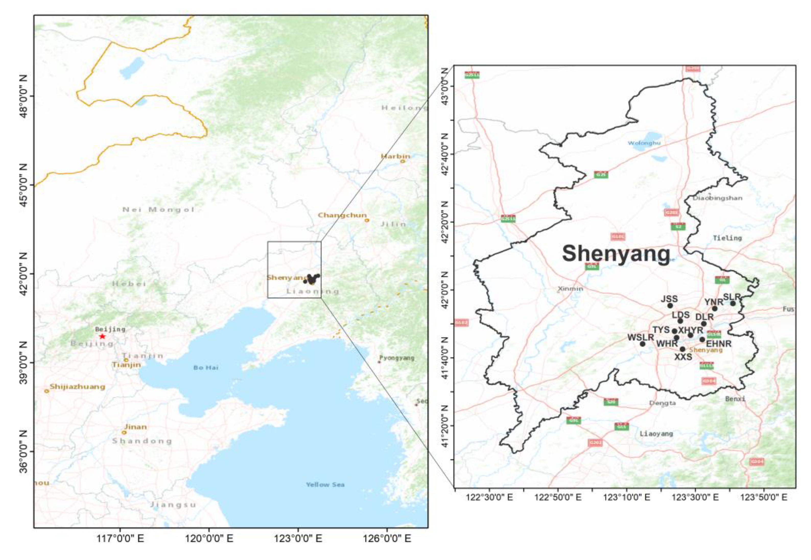
2.1. Research Area and Data Source

Shenyang (41°48′11.75” N, 123°25′31.18” E) is one of the mega-cities in China and is located in the center of Northeast Asian Economic Circle and the Bohai Economic Circle. The total area of the city is about 13,000 square kilometers [30]; the urban area is about 3495 square kilometers. The permanent resident population of the city in 2018 was 8.316 million at the time, and the GDP in the same year was 61.19 billion. It features a temperate, semi-humid continental climate, with an annual average temperature of 6.2–9.7 °C and an annual precipitation of about 600–800 mm. Under the influence of the monsoon, the precipitation is mostly concentrated in summer; the temperature difference is large; the four seasons are distinct; and the winter time is longer.
On the basis of the Shenyang Atmospheric Environmental Quality Bulletin, in 2019, the annual average concentrations of PM10 and PM2.5 in Shenyang’s urban ambient air were 77 μg·m−3 and 43 μg·m−3, respectively. All exceeded the second-class national ambient air quality standard (PM10: 70 μg·m−3 and PM2.5: 35 μg·m−3). The annual average concentrations of SO2 and NO2 were 21 μg·m−3 and 36 μg·m−3, respectively, which did not exceed the national second-class quality standard (SO2: 60 μg·m−3 and NO2: 40 μg·m−3). The average 95th percentile concentration of CO in 24 h was 1.9 mg·m−3. The 90th percentile concentration of the maximum 8 h moving average of O3 was 155 μg·m−3.
In this study, the mass concentrations of six pollutants from 1 January 2017 to 31 December 2019 were collected from 11 air quality monitoring stations in Shenyang (Figure 1). The hourly monitoring data of pollutants at 11 monitoring stations can be obtained from the website https://www.aqistudy.cn/historydata/. The instruments and analytical methods used to measure the concentrations of six pollutants were as follows: CO—gas filter correlation infrared absorption method 48i CO analyzer; SO2—UV fluorescence type 43i sulfur dioxide analyzer; NO2—chemiluminescence 42i NOx analyzer; O3—ultraviolet fluorescence 49i ozone analyzer; PM2.5—β-ray + dynamic heating system combined with light scattering method 5030i PM2.5 atmospheric particulate concentration monitor; and PM10—β-ray method 5014i type PM10 atmospheric particulate concentration monitor. The concentration data of CO, SO2, NO2, PM2.5, and PM10 used in this study were hourly monitoring values, and O3 concentration data were 8 h moving averages. According to the “Monitoring Regulation for Ambient Air Quality” (HJ/T193-2005) [31], all measured data were screened to exclude abnormal values and ensure data quality. The calculation, statistical analysis and evaluation of effective monitoring data referred to the “Ambient Air Quality Standard” (GB3095-2012) and Technical Regulation for Ambient Air Quality Assessment (Trial) (HJ663-2013) [32]. Among the 11 monitoring stations, Senlin Road (SLR) is located in a first-class ambient air functional area, and East Hunnan Road (EHNR), Xinxiu Street (XXS), Dongling Road (DLR), Lingdong Street (LDS), Wenhua Road (WHR), Xiaoheyan Road (XHYR), Taiyuan Street (TYS), Jingshen Street (JSS), West Shenliao Road (WSLR) and Yunong Road (YNR) are all located in second-class ambient air functional areas. The meteorological data of wind speed (km/h), air temperature (°C) and air pressure (hpa) in 2019 were from Shenyang Meteorological Monitoring Station, which can be obtained from the website http://data.cma.cn/. According to the “Division of Climate Season” (QX/T152-2012) [33], the seasons of Shenyang in 2019 were divided into four parts: spring (14 April to 20 June), summer (21 June to 28 August), autumn (29 August to 13 October) and winter (14 October to 13 April).

2.2. Analysis of Spatio-Temporal Distribution Characteristics

The spatial distribution of pollutant concentration was analyzed by sufer 15 (Golden Software, Golden, CO, USA). The spatial interpolation analysis was carried out for the annual average concentrations of pollutants in 11 monitoring stations, and Kriging interpolation method was used. The ward method in SPSS 26 (Statistical Product and Service Solutions) software was used for systematic cluster analysis, and the tree diagram of the ward connection was made by taking the square Euclidean distance as the interval to further verify the difference of the spatial distribution of pollutant concentration. Based on the pollutant concentrations of 11 monitoring sites, they were divided into different categories. The concentrations of pollutants at the monitoring points in the same group were similar, and there were some differences between different groups. At the same time, the seasonal, monthly and diurnal variations of different pollutants were analyzed.

2.3. Meteorological Element Analysis and Backward Trajectory Analysis

There are two meteorological monitoring stations in Shenyang. In this study, the correlations between six pollutants and air temperature (T), air pressure (P) and wind speed (WS) in 2019 were analyzed by the Pearson correlation coefficient method based on the meteorological data from the meteorological monitoring station close to the air quality monitoring station. In order to explore the differences of regional transport sources of air pollutants in different seasons in the main urban area of Shenyang, based on the pollutant concentration data in 2019, the HYSPLIT model developed by the National Oceanic and Atmospheric Administration (NOAA) (http://ready.arl.noaa.gov/HYSPLIT.php) was used to simulate the backward trajectory of 100 m height in the central urban area of Shenyang for 72 h, and the transport and diffusion orbits of atmospheric pollutants were analyzed [34].
In order to facilitate the analysis of the transport path of pollutants, the stepwise cluster analysis (SCA) algorithm was used to cluster the backward trajectories. In this algorithm, the trajectories with the closest spatial similarity were merged according to the transmission direction and the speed of each airflow track. After repeated calculation and merging, several representative clustering trajectories were finally obtained.
The calculation formula of SCA is as follows:
D = j = 0 t d j 2 ,
S P V A R = i = 1 x j = 0 t d i j 2 ,
T S V = S P V A R ,
where D is the distance between any two trajectories; t represents the trajectory transmission time; i is the backward trajectory number, i = 1,2,…,8760; j is the stop point number; x is the number of trajectories in the cluster; dj is the spatial distance between the jth stop points of the two trajectories; dij represents the spatial distance from the jth stop point in the ith backward trajectory to the corresponding stop point of the average trajectory; SPVAR is space variation of each group of trajectories; and TSV is total space variation.

3. Results

3.1. Analysis of Spatio-Temporal Distribution Characteristics of Six Air Pollutants

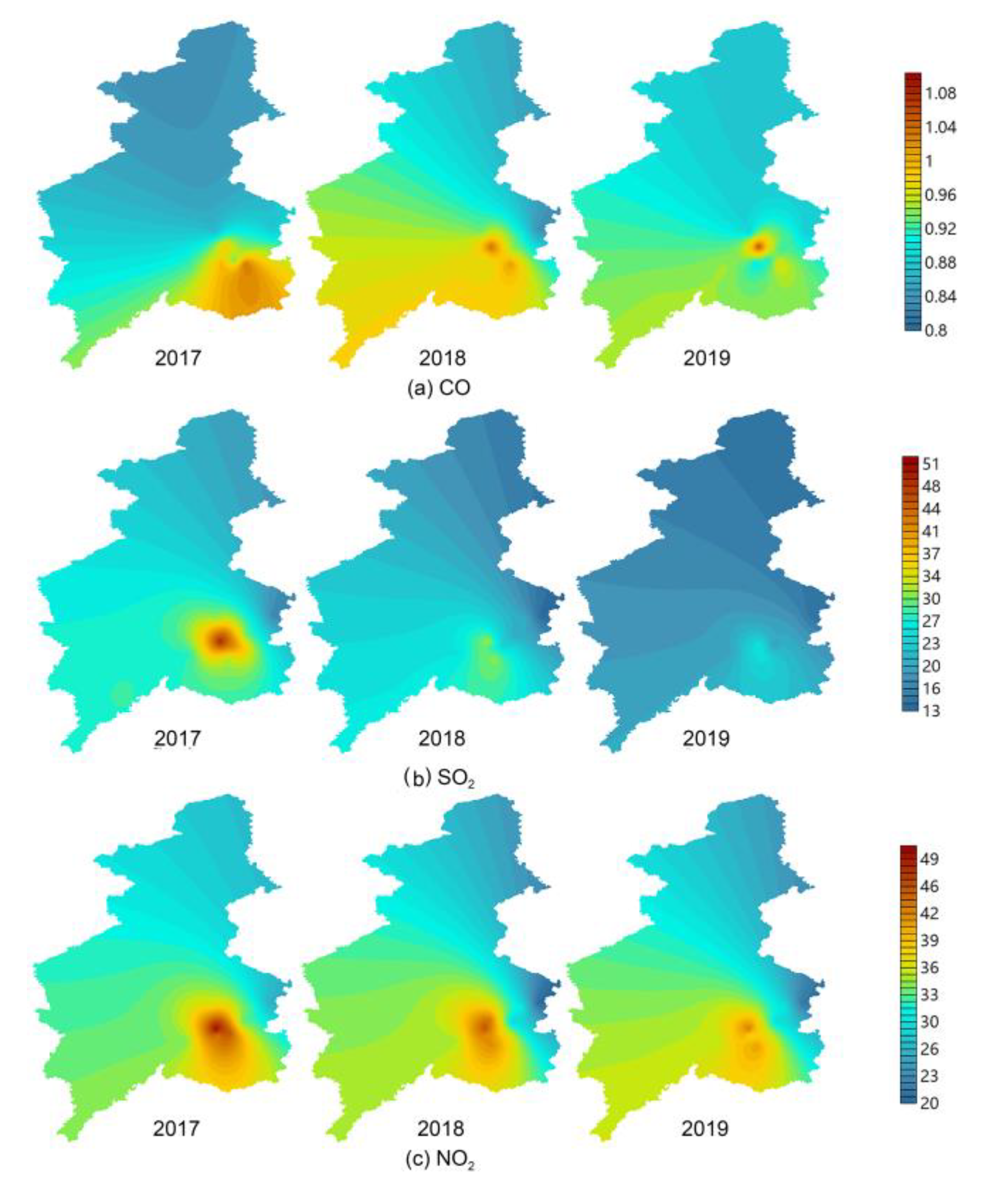
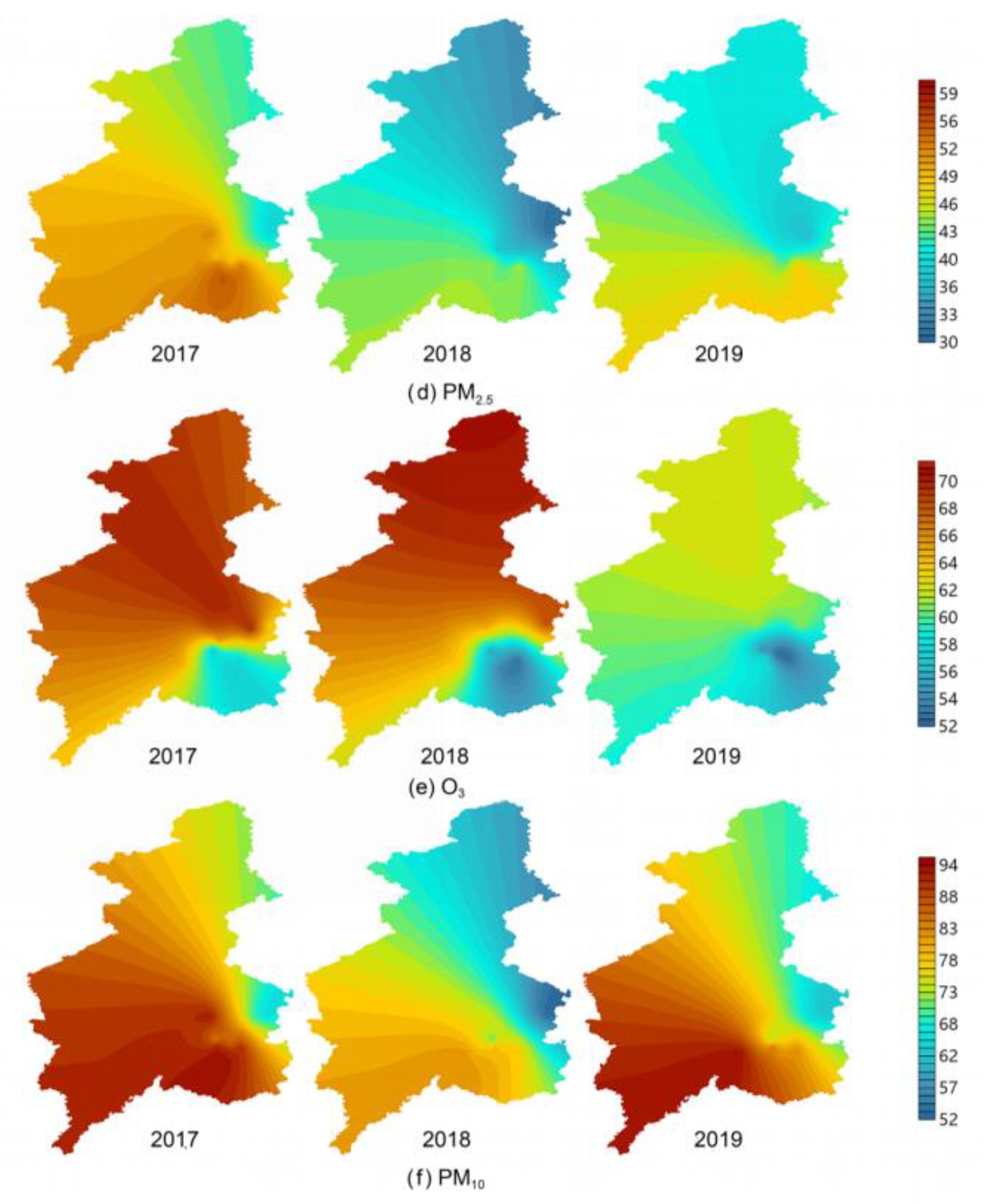
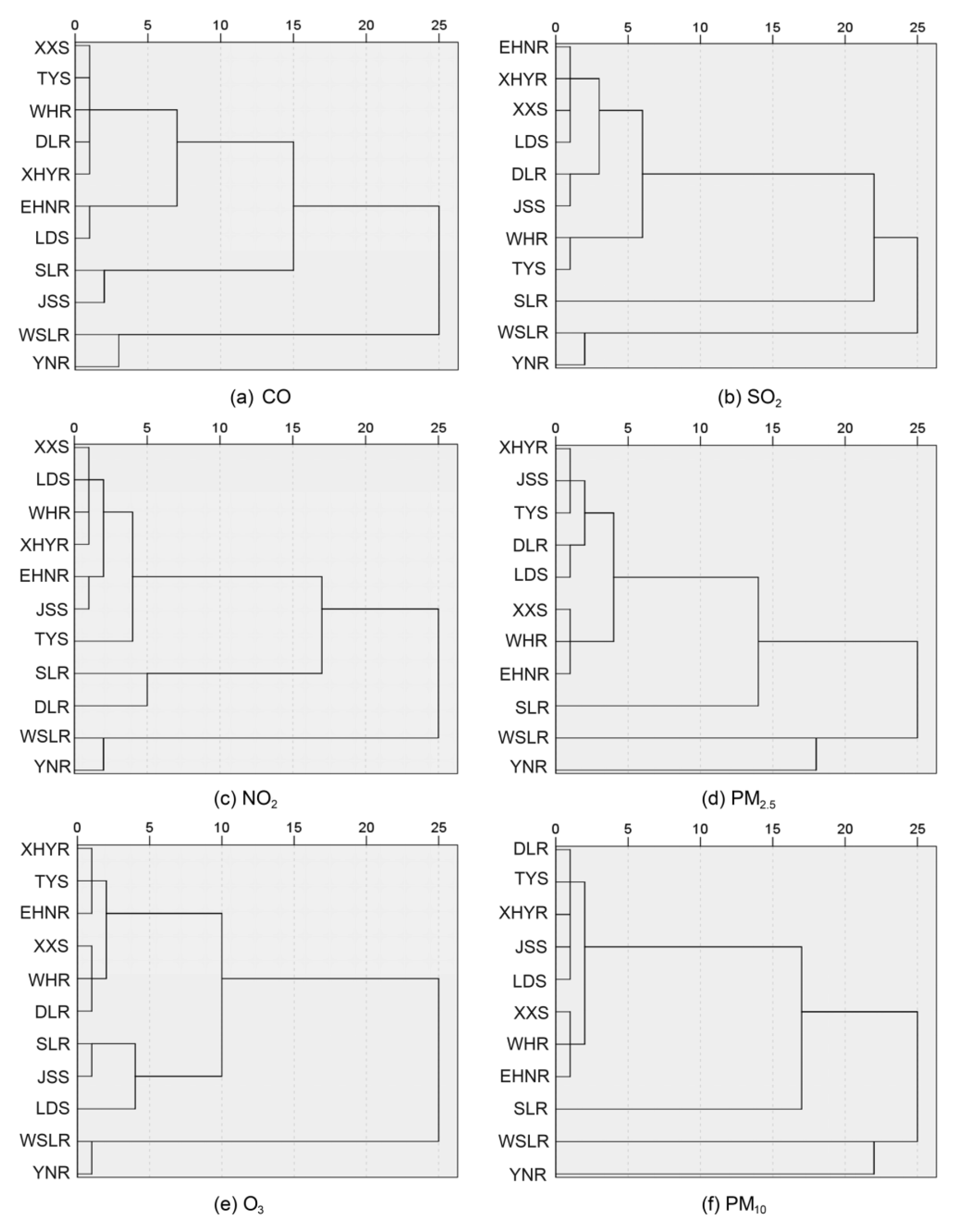
3.1.1. Difference in Spatial Distributions of Pollutant Concentrations

The spatial distributions of pollutant concentration are shown in Figure 2. The average annual mass concentrations of the six pollutants at the 11 monitoring sites in 2017–2019 are shown in Table S1. It was found that O3 concentration was higher in the northern region, and the concentration showed a trend of decreasing. The reason may be the rich vegetation coverage in the northern region and the poor vegetation coverage in the central city compared with the surrounding areas [35]. Vegetation is an effective barrier to some pollutants (SO2, NO2); however, it releases a large number of ozone precursors such as volatile organic compounds (VOCs), thereby increasing the ozone concentration [36,37,38,39]. The concentration of O3 in LDS decreased the most, at 17.94% (from 65.3 to 56.2 μg·m−3).
The concentrations of CO, SO2 and NO2 in the central urban area were higher than in the urban fringe area, as reported by Arain et al., and Dommen et al. [40,41]. The high concentration of CO in the central urban area may be due to the higher traffic flow in the urban center than in the marginal areas. CO emissions come from a large number of gasoline-driven private cars [42]. The low concentrations of SO2 and NO2 in the edge area may be related to the vegetation coverage mentioned in the previous paragraph [35]. The annual average concentration of CO increased first and then decreased. The concentration in 2019 was lower than that in 2017. The average concentrations of CO over three-years at EHNR and LDS were the highest, while the lowest were at SLR and JSS. The concentrations of SO2 and NO2 both decreased year by year. It is speculated that the changes of SO2 and NO2 were due to the implementation of central heating in northeast China in recent years, replacements of small boilers, the promotion of hot-spot co-production projects and the implementation of gas standards for coal burning, which reduced the consumption of coal burning and thus led to the reduction of pollutant emissions [43]. The SO2 concentrations in WHR and TYS were higher than in other monitoring sites, and the concentration in SLR was always the lowest. Compared with other sites, the NO2 concentration in SLR was the lowest. The low concentrations of SO2 and NO2 in SLR may be related to its location in the first-class ambient air functional area. The highest concentration of NO2 in monitoring stations was found in TYS for three consecutive years, which may be due to the dense population, large traffic flow and higher exhaust emissions at the TYS monitoring point [44]. The concentrations of SO2 and NO2 decreased the most in XHYR, at 52.7% (from 40.93 to 19.36 μg·m−3) and 17.8% (from 45.1 to 37.1 μg·m−3), respectively.
The concentrations of PM2.5 and PM10 in the southern region were higher than those in the northern region, which may be related to the fact that Tiexi (northeast old industrial base) was located in the southwest of Shenyang [45], where there are many anthropogenic emission sources. The average concentration in 2019 was lower than that in 2017. The concentrated high-value zones were located in EHNR, XXS, WSLR and WHR. The spatial distributions of PM10 and PM2.5 were similar to each other, which verifies that their pollution is similar [46,47,48].
Cluster analysis can aggregate indicators with similar characteristics into a group to determine the similarity between research objects [49,50]. According to the spatial distribution of pollutant concentration, we analyzed the distribution characteristics of each pollutant at different monitoring points. In order to more intuitively show the similarity between the monitoring stations and further verify the spatial distribution characteristics of pollutant concentration, the concentration of pollutants in each monitoring point was analyzed by cluster analysis. If there was similarity between two monitoring points, they were placed in the same group.
The results are shown in Figure 3. It can be seen that the results of cluster analysis were consistent with the results of spatial distribution. For example, based on the annual average concentration of pollutants, 11 monitoring stations were divided into four groups. The clustering results of SO2 were as follows: the first group: WSLR, YNR; second group: SLR; third group: WHR, TYS; fourth group: other monitoring points. The results of the spatial distribution showed that the concentration of SO2 was relatively high at the WHR and TYS and relatively low at the SLR. In cluster analysis, WHR and TYS were divided into a group and SLR was a group, which was consistent with the results of spatial analysis. In addition, the remaining eight monitoring points were further divided into two groups. When the CO clustering results were divided into four groups, the first group was WSLR, YNR; the second group was SLR, JSS (the results of the spatial distribution showed that CO concentrations in these two stations were relatively low); the third group was EHNR, LDS (the results of spatial distribution showed that CO concentration in these two stations was relatively high); and the fourth group was all other monitoring points.

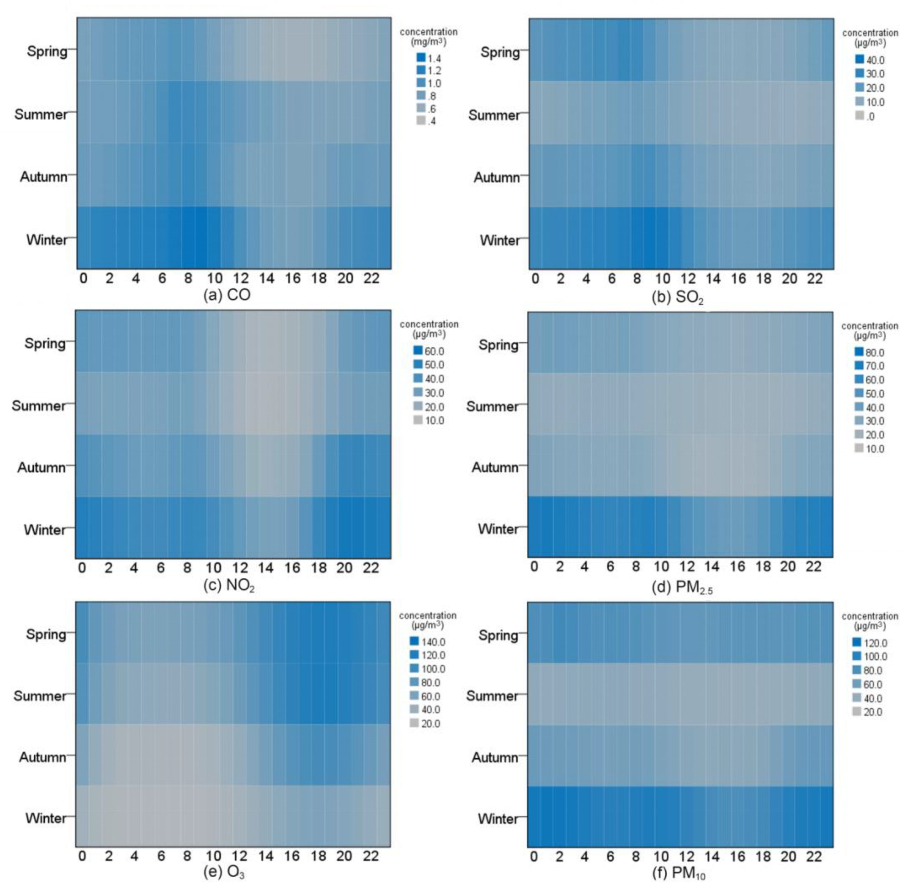
3.1.2. Seasonal Variation of Pollutant Concentrations

The analysis in the previous section shows that the annual average concentration change trend of each pollutant was different in 2017–2019. Therefore, we selected the latest data of 2019 to analyze the seasonal variation trend of pollutants, hoping to better express the current situation. Figure 4 shows the seasonal variations of the six pollutants’ concentrations in Shenyang, which are similar to the variations of most cities in China [51]. The concentration of O3 was the highest in spring and lowest in winter. The difference of O3 concentration between seasons may be due to the lower radiation levels in winter than other seasons and the gradual accumulation of precursors such as NO, NO2 and VOCs in winter (Figure 4, the concentration of NO2 was higher in winter), which resulted in a large amount of O3 production during the enhancement of solar radiation in spring [52,53,54]. The difference between the average concentrations in spring and winter was 51.5 μg·m−3. The analysis of the variation of O3 concentration between seasons also revealed that it showed typical diurnal variation in urban areas [55]; the daily high value appeared at 15:00–20:00, and the low value appeared mostly at 3:00–9:00.
The seasonal average concentration of NO2 showed a trend of winter > autumn > spring > summer, which was consistent with the relevant study at northern midlatitudes [56,57]. The high concentration in winter may be due to people relying more on transportation than walking to get around, resulting in increased traffic emissions. The difference between winter and summer was 17.8 μg·m−3. The daily low concentration appeared at 13:00–17:00.
The seasonal average concentrations of SO2, PM10 and PM2.5 were all in the order of winter > spring > autumn > summer, which was similar to the seasonal variation of Wuhan, China and Kolkata, India [58,59]. The height of the mixed layer was high in summer, when the atmospheric instability and the increase of precipitation were conducive to the diffusion of some air pollutants. The difference between the average seasonal concentration in winter and summer was 23 μg·m−3. The daily concentration of SO2 was relatively high from 7:00 to 9:00, and relatively low from 13:00 to 21:00. The seasonal average concentration of PM2.5 was similar in spring, summer and autumn, which was consistent with the relevant research results [60]. In winter, the concentration of PM2.5 was significantly higher under the influence of heating, with a difference of 34.3 μg·m−3 from the average concentration in summer. The PM2.5 concentration was relatively low at 14:00–17:00. Similarly to the related studies, the concentration of PM10 was significantly higher in winter and spring [61]. Coal combustion for heating purposes and dust weather caused relatively high concentrations in winter and spring. The climate background of rising temperature and increasing wind speed in spring is conducive to the formation of dust weather, which leads to the ground particles being drawn into the air [62]. The seasonal average concentration difference of PM10 between winter and summer was 51.5 μg·m−3, and the daily change trend was similar to that for PM2.5. The seasonal average concentration of CO was relatively low in spring and summer and high in winter. The concentration from 7:00 to 10:00 was relatively high, and that from 15:00 to 18:00 was relatively low.

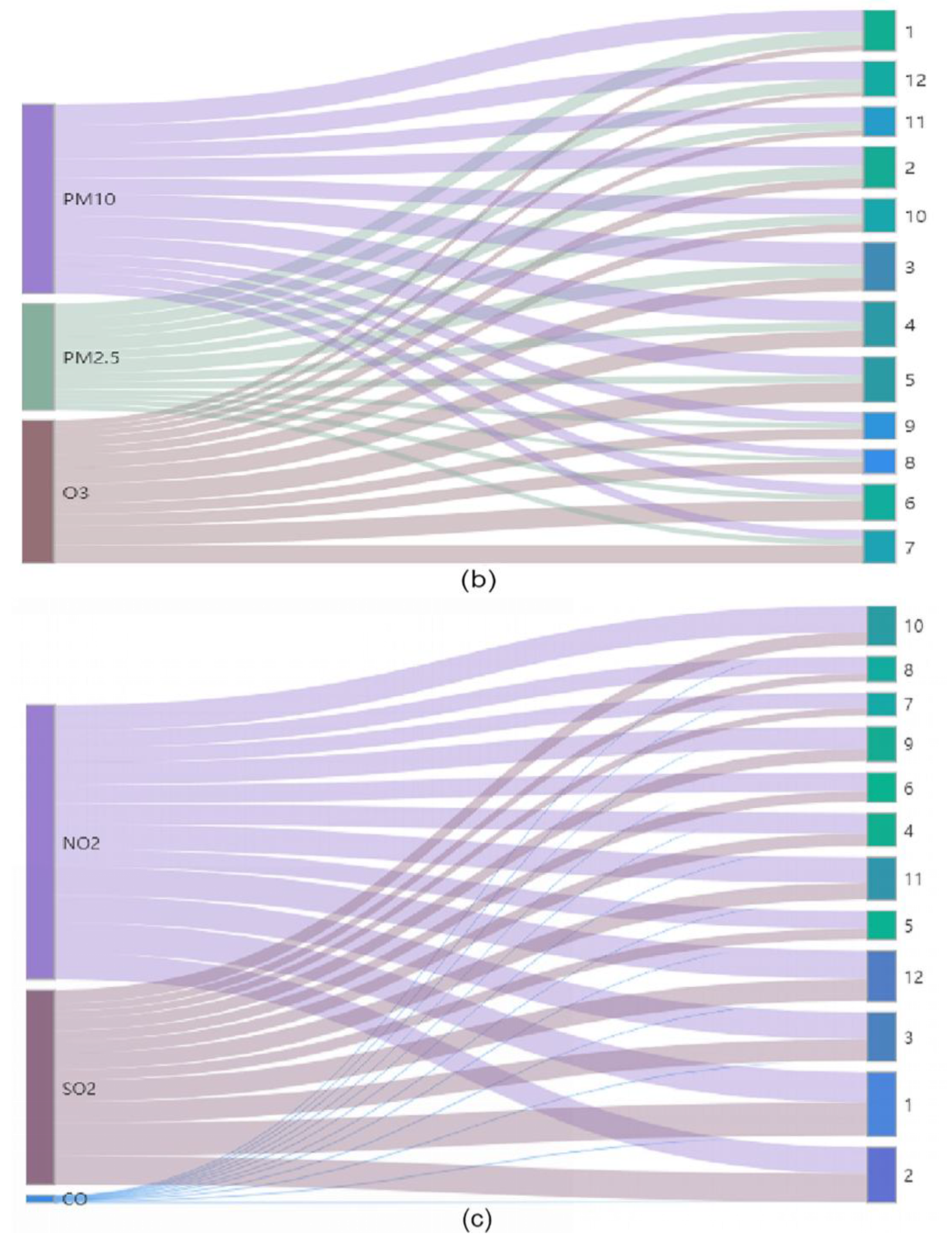
3.1.3. Monthly Variation of Pollutant Concentrations

The monthly average concentration changes of the six pollutants in Shenyang from 2017 to 2019 are shown in the Sankey diagram (Figure 5). The left column shows pollutants and the right column shows the period of January to December. The advantage of using a Sankey chart is that it can show the data flow of pollutant concentration in 12 months. At the same time, according to the length of the month bar on the right, the months with higher accumulated concentrations of six pollutants in a year can be visually displayed; the longer the column, the higher the cumulative concentration. On the whole, the cumulative concentrations of the six pollutants were highest in March, followed by January and February, and the cumulative concentrations in July, August, September and November were relatively low (Figure 5a). The results were consistent with the study of Shen et al., regarding the monthly changes of six pollutants in China from 2015 to 2018 [51].
In winter, coal combustion for heating purposes leads to increased emissions of pollutants such as SO2, PM10 and PM2.5, while increased rainfall in July and August inhibits pollutant transport, accelerates pollutant deposition and indirectly improves air quality. The concentrations of SO2 were relatively high in January and February, at 54.3 and 45.7 μg·m−3 respectively. In July and August, the concentrations were” relatively low, at 12.1 and 12.9 μg·m−3 respectively. The high values of NO2 were distributed in January–March and October–December, with the highest value of 49.5 μg·m−3 in January and the lowest in July (25.1 μg·m−3).
The concentrations of PM10 and PM2.5 were higher in January and March and lower in July–September. The concentration of PM10 was the highest in March (107.6 μg·m−3) and the lowest in August (39.8 μg·m−3), while the concentration of PM2.5 was the highest in January (68.5 μg·m−3) and the lowest in August (21.0 μg·m−3). Figure 5b shows that the high concentrations of O3 occurred in May–July, and the low concentrations appeared in January, November and December, as reported by Yang et al. and Wang et al. [63,64]. The value was highest in June (97.1 μg·m−3) and lowest in December (24.2 μg·m−3). The number of hours with sunshine in June was relatively high, and the degree of solar radiation was strong, which led to a high concentration of O3 [65].

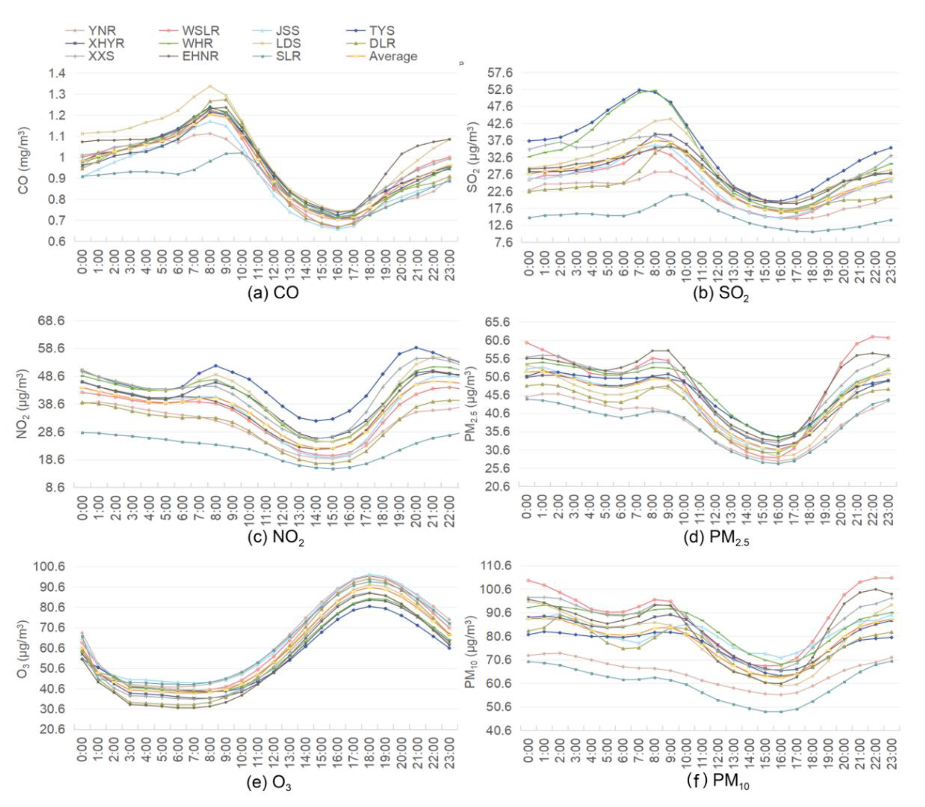
3.1.4. Diurnal Variation of Pollutant Concentrations

The daily 24-h concentration changes of the six pollutants at 11 monitoring points are shown in Figure 6. The results showed that the diurnal concentration variations of O3, CO, and SO2 exhibited a “single peak,” while others showed a “double peak and double valley.” The hourly average concentrations of CO, SO2, NO2, PM10 and PM2.5 at the SLR monitoring sites located in the first-class ambient air functional areas all met the first-class concentration standard in the “Environmental Air Quality Standard” (GB3095-2012), while the other 10 monitoring sites met the corresponding secondary concentration standard in the second-class areas (there is no hourly average concentration standard for PM10 and PM2.5 in the “Environmental Air Quality Standard” (GB3095-2012); therefore, it was replaced by three times the 24 h average concentration standard). The concentrations of pollutants in SLR were generally the lowest, which may have been due to the fact that they were located in the first-class ambient air functional areas and were less affected by human activities.
The peak value of O3 appeared at 18:00 in 11 monitoring points. The valley value of the YNR monitoring point appeared at 5:00, the TYS valley value appeared at 8:00, the valley value for DLR and SLR appeared at 6:00 and the valley value of all other points appeared at 7:00. The concentration of O3 began to increase in the morning, which was mainly due to the appearance of a large number of precursors in the early peak period, coupled with the increase of light, which promoted the photochemical reaction. Affected by the early peak of traffic flow, the peak value of CO appeared at 8:00–10:00 and the lowest value appeared at 16:00. The peak value of SO2 appeared between 7:00 and 10:00, and the valley value appeared between 16:00 and 18:00.
It is consistent with the relevant research of other inland cities (Dezhou, Liaocheng, Heze, and Jining) in China [66]; the first peak of NO2 for most points was between 7:00 and 8:00 and the late peak was between 20:00 and 21:00. The concentration of the first peak was generally lower than that of the late peak. The emergence of the first peak may be related to human activities. It was at the peak of people’s travel, with more vehicle exhaust emissions. The second peak may have been due to the decreased O3 concentration after 18:00, the decreased NO2 consumption and the increased number of trucks in the city at night.
The daily concentration variation trend of PM10 and PM2.5 was basically the same, and the early peak basically appeared at 8:00–9:00. It was speculated that the reason for this was related to the atmospheric stability and the increase of human activities in this period [67]. Then, the concentration showed a downward trend; after falling to the valley value at about 16:00, the concentration began to increase continuously. After 22:00, the concentration entered the second high-value area, which lasted until about 1:00 the next day. It is speculated that the emergence of the second high-value area was mainly affected by entertainment such as barbecues at night. Although the concentration decreased between the second peak and the first peak (at night), the decrease was not significant, which may be related to the fact that most large diesel vehicles drive into urban areas at night [39].

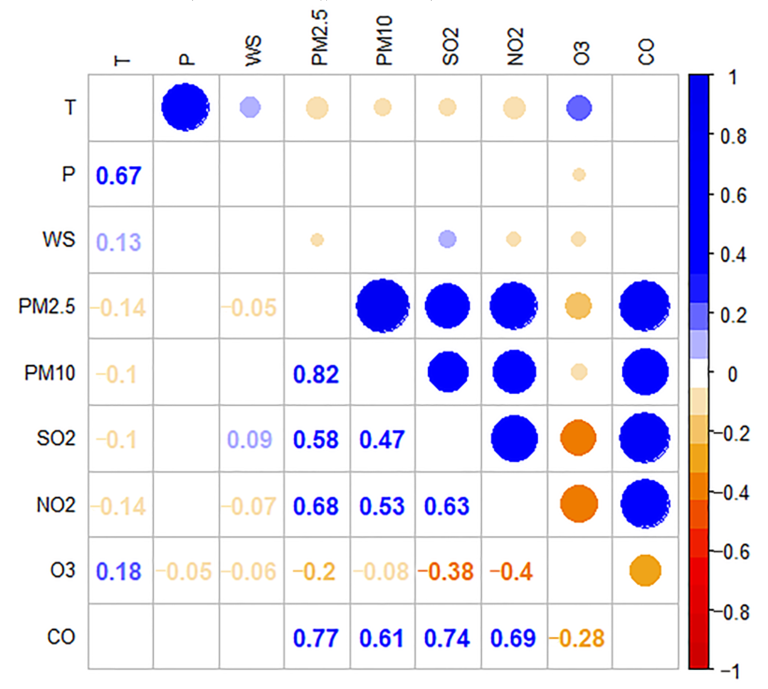
3.2. Influence of Meteorological Factors on Pollutant Concentrations

Meteorological factors play an important role in the formation and dispersion of pollutant concentration [68]. This study analyzed the correlations between the six air pollutants and air temperature, air pressure and wind speed in 2019 in Shenyang (Figure 7). Similarly, in order to show the current situation better, we still selected the data in 2019. We set the confidence interval level to 99%, and the correlation degree was expressed by the Pearson correlation coefficient r.
The results showed that the concentrations of CO, SO2, NO2, PM10 and PM2.5 had positive correlations (the P values of the five pollutants were all less than 0.01) which were similar to the correlation between air pollutions in Jiangsu Province [69]. This may be related to the fact that there were many industrial point sources in Shenyang, and the most primary pollutant came from these industrial point sources. CO was strongly positively correlated with SO2 (r = 0.744), NO2 (r = 0.692), PM10 (r = 0.605) and PM2.5 (r = 0.770). The correlation coefficients of NO2 with SO2, PM10 and PM2.5 -were 0.625, 0.526 and 0.677, respectively. The correlation coefficient of PM2.5 and PM10 was as high as 0.822. This shows that these fractions were emitted from a similar emission source. There was a negative correlation between O3 and the other five pollutants (the P values of O3 with the other five pollutants were all less than 0.01), which was consistent with the study in Delhi, India [70]. O3 had a strong negative correlation with SO2 (r = −0.379) and NO2 (r = −0.403), which was consistent with the results of the above seasonal and daily variation curves of pollutant concentration. The concentrations of SO2 and NO2 were lower in the period with high O3 concentration.
There was a positive correlation between temperature and O3 (p < 0.01, r = 0.184). The increase of O3 concentration with the increase of temperature is consistent with most research outcomes [71,72] because the temperature increases at the same time as strong solar radiation, accelerating the photochemical reaction. The negative correlation between temperature and the other five pollutants may be due to the low air temperature increasing the activity of emission sources such as fuel combustion for heating purposes. Thus, the lower the air temperature, the higher the concentrations of pollutants, because the intensity of emissions from anthropogenic sources increases [73]. In addition, the stability of atmospheric stratification decreases with the increase of temperature. This is conducive to the development of convective conditions near the ground and the vertical movement of the atmosphere. Therefore, a high temperature provides favorable conditions for pollutant diffusion. There was no significant correlation between air pressure and pollutants, resembling the research result discovered by Lv et al. [74]. Wind speed has a negative correlation with NO2, PM2.5 and O3. The annual average wind speed was 7.96 km/h. The increase of wind speed in a certain range is conducive to the transportation of pollution and does not easily raise dust, thereby reducing the concentrations of pollutants [75].

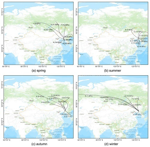
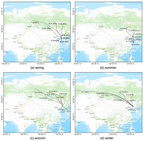
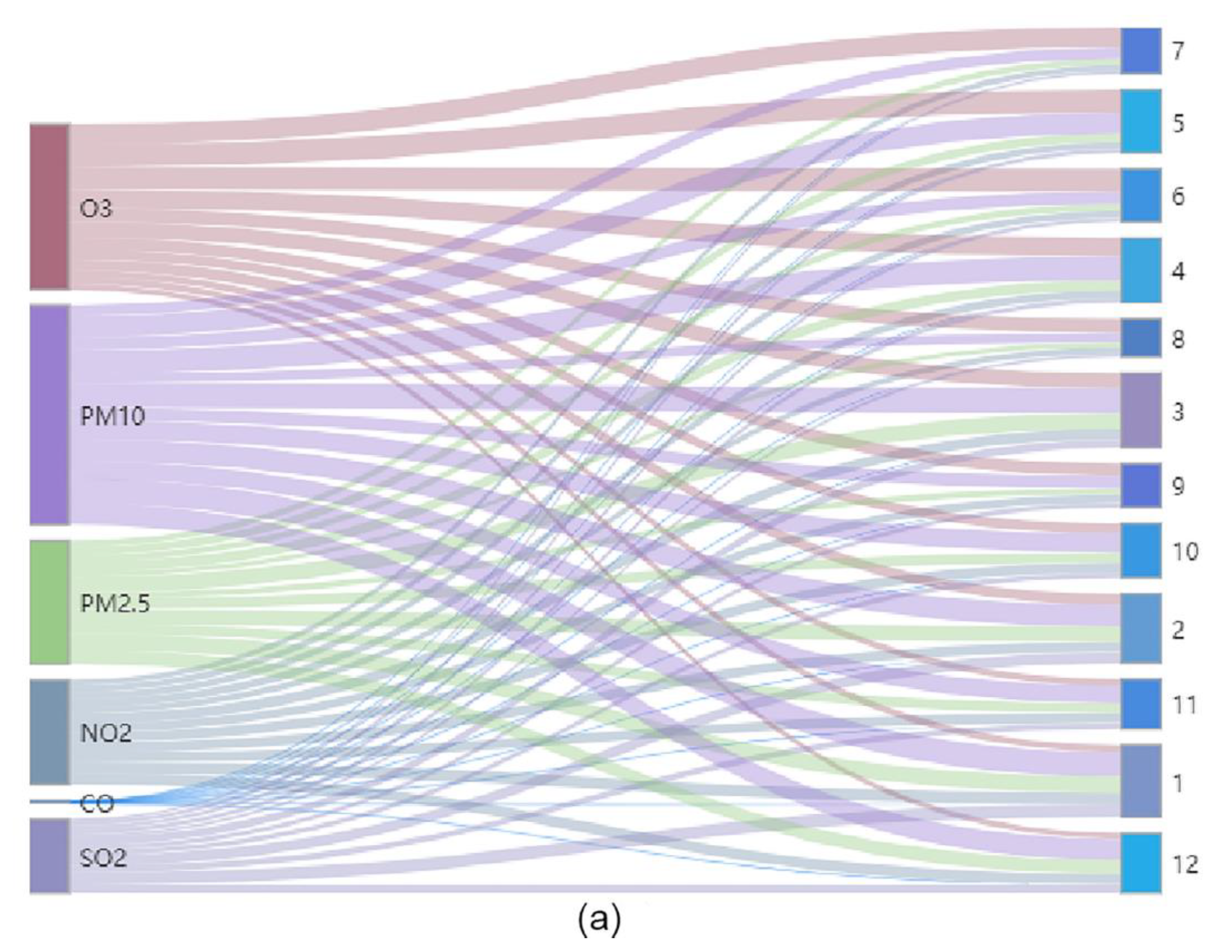
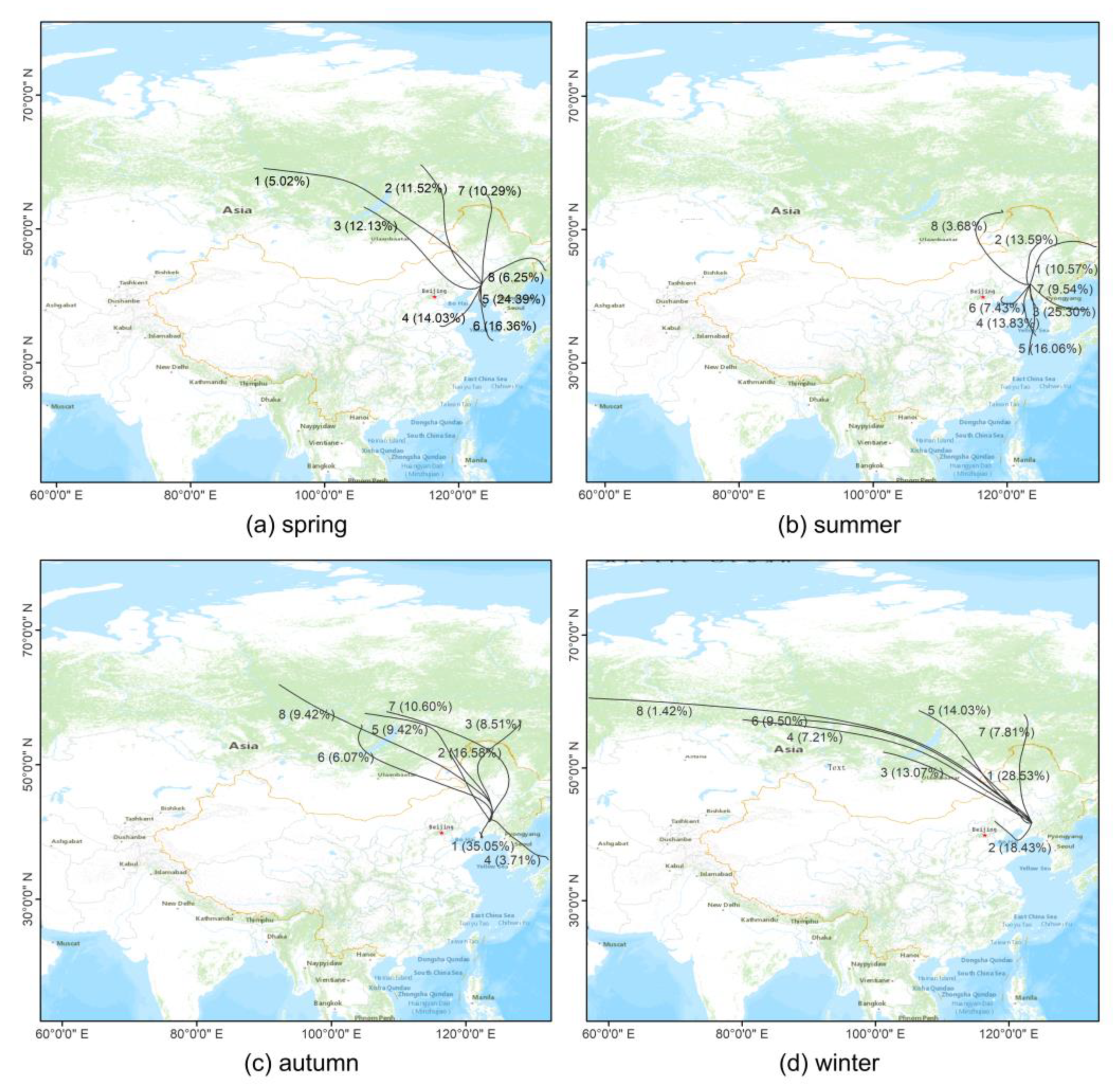
3.3. Backward Trajectory Clustering Analysis

The starting point of the simulation was the TYS monitoring point, close to the center of the main urban area of Shenyang. Taiyuan Street is located in the bustling business district in the center of Shenyang, and the above analysis results showed that the air pollution in TYS station was the most serious of the 11 monitoring sites. In order to facilitate the analysis of the backward trajectory of the airflow, this study made a cluster analysis of all the tracks affecting the site and divided them into eight categories. According to the results of clustering, the length of each track and its proportion to the total trajectory were calculated. An air flow with a higher percentage of the total trajectory has a great influence on air quality. Northeast China is a region with severe haze pollution, and the higher pollutant concentration in winter was mainly affected by coal combustion for heating purposes, as shown in the previous analysis. Therefore, PM2.5 and SO2 mass concentrations corresponding to each trajectory were calculated. The results are shown in Figure 8 and Table 1.
In all the trajectories of the four seasons, the average mass concentrations of SO2 and PM2.5 were the lowest in summer and the highest in winter, which was consistent with the analysis results in Section 3.1.2. Compared with other seasons, the air transport distance in winter was longer, which may be related to the winter monsoon [76]. In spring and summer, the coastal air current has a great influence on pollutant concentrations. In spring, the air flow from the southeast direction accounted for the largest proportion, accounting for 40.75% of the total air flow from the Yellow Sea to Shenyang via other cities in Liaoning Province. Cluster 5 has the highest probability of occurrence and has the greatest impact on the air quality of the study area. The average mass concentrations of SO2 and PM2.5 were 13.30 and 27.72 μg·m−3, respectively. The results show that the highest concentrations of SO2 and PM2.5 were in cluster 4, which came from Shandong Province and reached the study area through the Yellow Sea. The high concentrations of the two pollutants on the trajectory may be due to the developed industry, large population and more anthropogenic sources in Shandong Province. In summer, the southward air flow track accounts for the highest proportion, at 55.19%; cluster 3 has the highest probability of occurrence. The average mass concentrations of SO2 and PM2.5 were 8.66 and 19.89 μg·m−3, respectively. Cluster 2 had the highest concentration of SO2 and cluster 4 has the highest concentration of PM2.5.
Under the influence of the semi-permanent cold high pressure in the Mongolia–Siberia region, the pollution mainly came from northwest airflow in autumn and winter, and the pollutants reached the study area through Mongolia, Inner Mongolia and other places. The northwest track accounts for 52.72% in autumn and 73.76% in winter. The desert area of Mongolia and Inner Mongolia is large, and the airflow from the northwest comes from close to the desert, so transports more dust aerosols in the transportation process. In addition, the northwest direction airflow path area’s agriculture is more developed, and crop burning in the open air produces is more common. At the same time, these areas are cold in winter, and the demand for coal for heating is greater. Therefore, more pollutants were carried in the air transport process, and the pollutant concentrations were higher in winter than in other seasons. In autumn, the average SO2 concentration of all tracks was 13.14 μg·m−3, and the average PM2.5 mass concentration was 20.15 μg·m−3. In winter, the average SO2 concentration of all tracks was 48.18 μg·m−3, and the average PM2.5 mass concentration was 22.62 μg·m−3. Affected by the sea–land breeze circulation, the air quality in the study area was affected by air flow trajectory 1 in autumn and air flow trajectory 2 in winter.

4. Conclusions

This work presents an in-depth study of the characteristics of pollutants in Shenyang and the purpose was to provide scientific support to make an effective air pollution control plan for Shenyang city and other similar urban areas. The results were as follows:
(1)
Affected by vegetation coverage, the concentrations of CO, SO2, NO2, PM10, and PM2.5 in the northern part of Shenyang were relatively low, while the trend of O3 concentration was the inverse. The high concentrations of CO, SO2, and NO2 were located in the central urban area. Because Tiexi (northeast old industrial base) was located in the southwest, the high concentrations area of PM10 and PM2.5 were located in the southwest.
(2)
Affected by coal combustion for heating purposes and rainfall, the accumulated concentrations of the six pollutants were higher from January to March and lower from July to September and November. In terms of the daily variation characteristics, the concentrations of CO, SO2, and O3 were of the “single peak” type, while NO2, PM10, and PM2.5 were of the “double peak and double valley” type. The study area belongs to the northeast old industrial base, with many industrial point sources. There was a significant positive correlation between CO, NO2, SO2, PM2.5, and PM10. Because the precursors were consumed and produced by photochemical reactions, the concentrations of NO2 and O3 showed a significant negative correlation. Low temperature increases the activity of emission sources; thus, the temperature was negatively correlated with the concentration of most pollutants.
(3)
The airflow transport distance was longer in winter due to the influence of the winter monsoon. The pollution in the main urban area in spring and summer was mainly affected by the ocean current from the Yellow Sea. In summer, the airflow pollution of SO2 and PM2.5 mainly originated in Shandong Province. Affected by the semi-permanent cold high in Mongolia–Siberia, the regional transport of pollutants in autumn and winter was mainly affected by the northwest airflow. Because the northwest airflow path area was close to the desert and the low temperature in winter leads to more anthropogenic emissions, the concentration of pollutants was highest in winter.
Overall, the spatial distributions of pollutant concentrations in this study area are similar to those in Changchun, Lanzhou, Toronto (Canada) and Lombardy (Italy) [39,40,41,45]; in terms of temporal variation, the results of this study are consistent with the previous studies in most parts of China (Fen Wei Plains, Sichuan Basin, Yangtze River Delta, Pearl River Delta, eastern Jianghan Plains) [51,58,60,63,64], Israeli and Kolkata (India) [56,59]; the conclusions of the study on the correlations between pollutant concentrations are similar to those in Jiangsu Province and Delhi (India) [69,70]; the correlations between pollutant concentration and meteorological factors are consistent with those in Yangtze River Delta, Beijing, Nagasaki (Japan) [71,72,74,75].

Supplementary Materials

The following are available online at https://www.mdpi.com/2073-4433/11/7/766/s1, Table S1: Mean annual concentrations of six pollutants at the 11 monitoring sites in 2017–2019.

Author Contributions

Data curation and methodology, C.F.; supervisors and directors, J.W.; conceptualization, original draft writing, review and editing, J.T.; field sampling and formal analysis, J.Q. All authors have read and agreed to the published version of the manuscript.

Funding

This research was funded by Ecology and Environment Department of Jilin Province. The project numbers are 2018-19 and 2019-08.

Acknowledgments

The authors would like to thank Shenyang ecological environment monitoring center of Liaoning Province for supporting us. Additionally, the authors would like to thank the group members of Laboratory 537 and 142 of Jilin University.

Conflicts of Interest

The authors declare no conflict of interest.

References

  1. Brauer, M.; Freedman, G.; Frostad, J.; van Donkelaar, A.; Martin, R.V.; Dentener, F.; Dingenen, R.; Estep, K.; Amini, H.; Apte, J.S.; et al. Ambient Air Pollution Exposure Estimation for the Global Burden of Disease 2013. Environ. Sci. Technol. 2016, 50, 79–88. [Google Scholar] [CrossRef] [PubMed]
  2. Cohen, A.J.; Brauer, M.; Burnett, R.; Anderson, H.R.; Frostad, J.; Estep, K.; Balakrishnan, K.; Brunekreef, B.; Dandona, L.; Dandona, R.; et al. Estimates and 25-year trends of the global burden of disease attributable to ambient air pollution: An analysis of data from the Global Burden of Diseases Study 2015. Lancet 2017, 389, 1907–1918. [Google Scholar] [CrossRef] [Green Version]
  3. Di, Q.; Wang, Y.; Zanobetti, A.; Wang, Y.; Koutrakis, P.; Choirat, C.; Dominici, F.; Schwartz, J.D. Air Pollution and Mortality in the Medicare Population. N. Engl. J. Med. 2017, 376, 2513–2522. [Google Scholar] [CrossRef] [PubMed]
  4. Kan, H.; Chen, R.; Tong, S. Ambient air pollution, climate change, and population health in China. Environ. Int. 2012, 42, 10–19. [Google Scholar] [CrossRef] [PubMed]
  5. Kim, K.H.; Jahan, S.A.; Kabir, E. A review on human health perspective of air pollution with respect to allergies and asthma. Environ. Int. 2013, 59, 41–52. [Google Scholar] [CrossRef]
  6. Hoek, G.; Krishnan, R.M.; Beelen, R.; Peters, A.; Ostro, B.; Brunekreef, B.; Kaufman, J.D. Long-term air pollution exposure and cardio- respiratory mortality: A review. Environ. Health 2013, 12. [Google Scholar] [CrossRef] [Green Version]
  7. Hu, J.; Huang, L.; Chen, M.; Liao, H.; Zhang, H.; Wang, S.; Zhang, Q.; Ying, Q. Premature Mortality Attributable to Particulate Matter in China: Source Contributions and Responses to Reductions. Environ. Sci. Technol. 2017, 51, 9950–9959. [Google Scholar] [CrossRef]
  8. Liu, J.; Han, Y.; Tang, X.; Zhu, J.; Zhu, T. Estimating adult mortality attributable to PM2.5 exposure in China with assimilated PM2.5 concentrations based on a ground monitoring network. Sci. Total Environ. 2016, 568, 1253–1262. [Google Scholar] [CrossRef]
  9. Clements, N.; Hannigan, M.P.; Miller, S.L.; Peel, J.L.; Milford, J.B. Comparisons of urban and rural PM10−2.5 and PM2.5 mass concentrations and semi-volatile fractions in northeastern Colorado. Atmos. Chem. Phys. 2016, 16, 7469–7484. [Google Scholar] [CrossRef] [Green Version]
  10. Van Donkelaar, A.; Martin, R.V.; Brauer, M.; Hsu, N.C.; Kahn, R.A.; Levy, R.C.; Lyapustin, A.; Sayer, A.M.; Winker, D.M. Global Estimates of Fine Particulate Matter using a Combined Geophysical-Statistical Method with Information from Satellites, Models, and Monitors. Environ. Sci. Technol. 2016, 50, 3762–3772. [Google Scholar] [CrossRef]
  11. Han, L.; Zhou, W.; Li, W.; Li, L. Impact of urbanization level on urban air quality: A case of fine particles (PM(2.5)) in Chinese cities. Environ. Pollut. 2014, 194, 163–170. [Google Scholar] [CrossRef] [PubMed]
  12. He, J.; Gong, S.; Yu, Y.; Yu, L.; Wu, L.; Mao, H.; Song, C.; Zhao, S.; Liu, H.; Li, X.; et al. Air pollution characteristics and their relation to meteorological conditions during 2014-2015 in major Chinese cities. Environ. Pollut. 2017, 223, 484–496. [Google Scholar] [CrossRef] [PubMed]
  13. Wang, B. The Spatial and Temporal Variation of Air Pollution Characteristics in China Adopting Air Pollution Index (API) Analysis. Master’s Thesis, Ocean University of China, Qingdao, China, 2008. [Google Scholar]
  14. Song, C.; Wu, L.; Xie, Y.; He, J.; Chen, X.; Wang, T.; Lin, Y.; Jin, T.; Wang, A.; Liu, Y.; et al. Air pollution in China: Status and spatiotemporal variations. Environ. Pollut. 2017, 227, 334–347. [Google Scholar] [CrossRef] [PubMed]
  15. Peng, J.; Chen, S.; Lü, H.; Liu, Y.; Wu, J. Spatiotemporal patterns of remotely sensed PM2.5 concentration in China from 1999 to 2011. Remote Sens. Environ. 2016, 174, 109–121. [Google Scholar] [CrossRef]
  16. World Health Organization. WHO Air Quality Guidelines for Particulate Matter, Ozone, Nitrogen Dioxide and Sulfur Dioxide (Global Update 2005): Summary of Risk Assessment; WHO Press: Geneva, Switzerland, 2005; pp. 9–11.
  17. Ma, Z.; Hu, X.; Sayer, A.M.; Levy, R.; Zhang, Q.; Xue, Y.; Tong, S.; Bi, J.; Huang, L.; Liu, Y. Satellite-Based Spatiotemporal Trends in PM2.5 Concentrations: China, 2004–2013. Environ. Health Perspect. 2016, 124, 184–192. [Google Scholar] [CrossRef] [Green Version]
  18. Li, T.; Wei, P.; Cheng, S.; Wang, W.; Xie, P.; Chen, Z.; Su, F.; ERen, Z. Air pollution characteristic and variation trend of Central Triangle urban agglomeration from 2005 to 2014. Chin. J. Environ. Eng. 2017, 11, 2977–2984. [Google Scholar]
  19. Nishanth, T.; Satheesh Kumar, M.K.; Valsaraj, K.T. Variations in surface ozone and NOx at Kannur: A tropical, coastal site in India. J. Atmos. Chem. 2012, 69, 101–126. [Google Scholar] [CrossRef]
  20. Ming, L.; Jin, L.; Li, J.; Fu, P.; Yang, W.; Liu, D.; Zhang, G.; Wang, Z.; Li, X. PM2.5 in the Yangtze River Delta, China: Chemical compositions, seasonal variations, and regional pollution events. Environ. Pollut. 2017, 223, 200–212. [Google Scholar] [CrossRef]
  21. Yao, L.; Yang, L.; Yuan, Q.; Yan, C.; Dong, C.; Meng, C.; Sui, X.; Yang, F.; Lu, Y.; Wang, W. Sources apportionment of PM2.5 in a background site in the North China Plain. Sci. Total Environ. 2016, 541, 590–598. [Google Scholar] [CrossRef]
  22. Zhou, J.; Wang, X.; Du, W.; Xue, Y. Analysis of Air Pollution Index and Its Influence Factors in Beijing. Environ. Monit. China 2015, 31, 53–56. [Google Scholar]
  23. He, J.; Yu, Y.; Xie, Y.; Mao, H.; Wu, L.; Liu, N.; Zhao, S. Numerical Model-Based Artificial Neural Network Model and Its Application for Quantifying Impact Factors of Urban Air Quality. Water Air Soil Pollut. 2016, 227. [Google Scholar] [CrossRef]
  24. Ma, Y.; Zhao, H.; Dong, Y.; Che, H.; Li, X.; Hong, Y.; Li, X.; Yang, H.; Liu, Y.; Wang, Y.; et al. Comparison of Two Air Pollution Episodes over Northeast China in Winter 2016/17 Using Ground-Based Lidar. J. Meteorol. Res. 2018, 32, 313–323. [Google Scholar] [CrossRef]
  25. Chen, W.; Liu, Y.; Wu, X.; Bao, Q.; Gao, Z.; Zhang, X.; Zhao, H.; Zhang, S.; Xiu, A.; Chen, T. Spatial and Temporal Characteristics of Air Quality and Cause Analysis of Heavy Pollution in Northeast China. Environ. Sci. 2019, 40, 4810–4823. [Google Scholar]
  26. Li, C.; Yuan, Z.; Wu, Y.; Ban, W.; Li, D.; Ji, C.; Gao, W. Analysis of Persistence and Intensification Mechanism of a Heavy Haze Event in Shenyang. Res. Environ. Sci. 2017, 30, 349–358. [Google Scholar]
  27. Hong, Y.; Li, C.L.; Li, X.L.; Ma, Y.J.; Zhang, Y.H.; Zhou, D.P.; Wang, Y.F.; Liu, N.W.; Chang, X.J. Analysis of Compositional Variation and Source Characteristics of Water-Soluble Ions in PM2.5 during Several Winter-Haze Pollution Episodes in Shenyang, China. Atmosphere 2018, 9, 280. [Google Scholar] [CrossRef] [Green Version]
  28. Yang, H.; Peng, Q.; Zhou, J.; Song, G.; Gong, X. The unidirectional causality influence of factors on PM2.5 in Shenyang city of China. Sci. Rep. 2020, 10, 8403. [Google Scholar] [CrossRef]
  29. Chang, D.; Song, Y.; Liu, B. Visibility trends in six megacities in China 1973–2007. Atmos. Res. 2009, 94, 161–167. [Google Scholar] [CrossRef]
  30. Sun, Y.; Zhou, Q.; Xie, X.; Liu, R. Spatial, sources and risk assessment of heavy metal contamination of urban soils in typical regions of Shenyang, China. J. Hazard. Mater. 2010, 174, 455–462. [Google Scholar] [CrossRef]
  31. Ministry of Ecology and Environment of the People’s Republic of China. HJ/T193-2005, Monitoring Regulation for Ambient Air Quality; China Environmental Science Press: Beijing, China, 2005.
  32. Ministry of Ecology and Environment of the People’s Republic of China. HJ 663-2013, Technical Regulation for Ambient Air Quality Assessment (on Trial); China Environmental Science Press: Beijing, China, 2013.
  33. China Meteorological Administration. Division of Climate Season QX/T 152—2012; China Meteorological Administration, Meteorological Publishing House: Beijing, China, 2012.
  34. Stein, A.F.; Draxler, R.R.; Rolph, G.D.; Stunder, B.J.B.; Cohen, M.D.; Ngan, F. NOAA’s hysplit atmospheric transport and dispersion modeling system. Bull. Am. Meteorol. Soc. 2015, 96. [Google Scholar] [CrossRef]
  35. Cao, Y.; Li, X.; Zhang, L. Analysis on dynamic evolution characteristics of vegetation in Liaoning Province from 2000 to 2014. Water Resour. Hydropower Eng. 2017, 48, 48–56. [Google Scholar]
  36. Yin, S.; Shen, Z.; Zhou, P.; Zou, X.; Che, S.; Wang, W. Quantifying air pollution attenuation within urban parks: An experimental approach in Shanghai, China. Environ. Pollut. 2011, 159, 2155–2163. [Google Scholar] [CrossRef] [PubMed]
  37. Vingarzan, R. A review of surface ozone background levels and trends. Atmos. Environ. 2004, 38, 3431–3442. [Google Scholar] [CrossRef]
  38. De Keijzer, C.; Agis, D.; Ambros, A.; Arevalo, G.; Baldasano, J.M.; Bande, S.; Barrera-Gomez, J.; Benach, J.; Cirach, M.; Dadvand, P.; et al. The association of air pollution and greenness with mortality and life expectancy in Spain: A small-area study. Environ. Int. 2017, 99, 170–176. [Google Scholar] [CrossRef] [PubMed]
  39. Wang, J.; Xie, X.; Fang, C. Temporal and Spatial Distribution Characteristics of Atmospheric Particulate Matter (PM10 and PM2.5) in Changchun and Analysis of Its Influencing Factors. Atmosphere 2019, 10, 651. [Google Scholar] [CrossRef] [Green Version]
  40. Arain, M.A.; Blair, R.; Finkelstein, N.; Brook, J.; Jerrett, M. Meteorological influences on the spatial and temporal variability of NO2 in Toronto and Hamilton. Can. Geogr. 2009, 53, 165–190. [Google Scholar] [CrossRef]
  41. Dommen, J.; Prevot, A.S.H.; Baertsch-Ritter, N.; Maffeis, G.; Longoni, M.G.; Gruebler, F.C.; Thielmann, A. High-resolution emission inventory of the Lombardy region: Development and comparison with measurements. Atmos. Environ. 2003, 37, 4149–4161. [Google Scholar] [CrossRef]
  42. Hassler, B.; McDonald, B.C.; Frost, G.J.; Borbon, A.; Carslaw, D.C.; Civerolo, K.; Granier, C.; Monks, P.S.; Monks, S.; Parrish, D.D.; et al. Analysis of long-term observations of NOx and CO in megacities and application to constraining emissions inventories. Geophys. Res. Lett. 2016, 43, 9920–9930. [Google Scholar] [CrossRef] [Green Version]
  43. Kong, S.F.; Ding, X.A.; Bai, Z.P.; Han, B.; Chen, L.; Shi, J.W.; Li, Z.Y. A seasonal study of polycyclic aromatic hydrocarbons in PM2.5 and PM2.5-10 in five typical cities of Liaoning Province, China. J. Hazard. Mater. 2010, 183, 70–80. [Google Scholar] [CrossRef] [PubMed]
  44. Wu, X.; Wu, Y.; Zhang, S.; Liu, H.; Fu, L.; Hao, J. Assessment of vehicle emission programs in China during 1998-2013: Achievement, challenges and implications. Environ. Pollut. 2016, 214, 556–567. [Google Scholar] [CrossRef] [PubMed]
  45. Zhang, K.; Yu, Z.; Gao, H.; Huang, T.; Ma, J.; Zhang, X.; Wang, Y. Gridded emission inventories and spatial distribution characteristics of anthropogenic atmospheric pollutants in Lanzhou valley. Acta Sci. Circumst. 2017, 37, 1227–1242. [Google Scholar]
  46. Yu, H.; Feng, J.; Su, X.; Li, Y.; Sun, J. A seriously air pollution area affected by anthropogenic in the central China: Temporal-spatial distribution and potential sources. Environ. Geochem. Health 2020. [Google Scholar] [CrossRef]
  47. Hu, J.; Wang, Y.; Ying, Q.; Zhang, H. Spatial and temporal variability of PM2.5 and PM 10 over the North China Plain and the Yangtze River Delta, China. Atmos. Environ. 2014, 95, 598–609. [Google Scholar] [CrossRef]
  48. Li, Y.; Chen, Q.; Zhao, H.; Wang, L.; Tao, R. Variations in PM10, PM2.5 and PM1.0 in an Urban Area of the Sichuan Basin and Their Relation to Meteorological Factors. Atmosphere 2015, 6, 150–163. [Google Scholar] [CrossRef] [Green Version]
  49. Sinha, S.; Basant, A.; Malik, A.; Singh, K.P. Iron-induced oxidative stress in a macrophyte: A chemometric approach. Ecotoxicol. Environ. Saf. 2009, 72, 585–595. [Google Scholar] [CrossRef] [PubMed]
  50. Xiong, Y.; McCormack, M.; Li, L.; Hall, Q.; Xiang, C.; Sheen, J. Glc-TOR signaling leads transcriptome reprogramming and meristem activation. Nature 2013, 496, 181–186. [Google Scholar] [CrossRef] [PubMed] [Green Version]
  51. Shen, F.; Zhang, L.; Jiang, L.; Tang, M.; Gai, X.; Chen, M.; Ge, X. Temporal variations of six ambient criteria air pollutants from 2015 to 2018, their spatial distributions, health risks and relationships with socioeconomic factors during 2018 in China. Environ. Int. 2020, 137, 105556. [Google Scholar] [CrossRef] [PubMed]
  52. Fernández-Fernández, M.I.; Gallego, M.C.; García, J.A.; Acero, F.J. A study of surface ozone variability over the Iberian Peninsula during the last fifty years. Atmos. Environ. 2011, 45, 1946–1959. [Google Scholar] [CrossRef]
  53. Xing, J.; Wang, S.X.; Jang, C.; Zhu, Y.; Hao, J.M. Nonlinear response of ozone to precursor emission changes in China: A modeling study using response surface methodology. Atmos. Chem. Phys. 2011, 11, 5027–5044. [Google Scholar] [CrossRef] [Green Version]
  54. Atkinson, R. Atmospheric chemistry of VOCs and NOx. Atmos. Environ. 2000, 34, 2063–2101. [Google Scholar] [CrossRef]
  55. Lal, S.; Naja, M.; Subbaraya, B.H. Seasonal variations in surface ozone and its precursors over an urban site in India. Atmos. Environ. 2000, 34, 2713–2724. [Google Scholar] [CrossRef]
  56. Boersma, K.F.; Jacob, D.J.; Trainic, M.; Rudich, Y.; DeSmedt, I.; Dirksen, R.; Eskes, H.J. Validation of urban NO2 concentrations and their diurnal and seasonal variations observed from the SCIAMACHY and OMI sensors using in situ surface measurements in Israeli cities. Atmos. Chem. Phys. 2009, 9, 3867–3879. [Google Scholar] [CrossRef] [Green Version]
  57. Lamsal, N.L.; Martin, R.V.; Donkelaar, A.; Celarier, E.A.; Bucsela, E.J.; Boersma, K.F.; Dirksen, R.; Luo, C.; Wang, Y. Indirect validation of tropospheric nitrogen dioxide retrieved from the OMI satellite instrument: Insight into the seasonal variation of nitrogen oxides at northern midlatitudes. J. Geophys. Res. Atmos. 2010, 115. [Google Scholar] [CrossRef]
  58. Zhang, F.; Wang, Z.W.; Cheng, H.R.; Lv, X.P.; Gong, W.; Wang, X.M.; Zhang, G. Seasonal variations and chemical characteristics of PM(2.5) in Wuhan, central China. Sci. Total Environ. 2015, 518, 97–105. [Google Scholar] [CrossRef] [PubMed]
  59. Karar, K.; Gupta, A.K. Seasonal variations and chemical characterization of ambient PM 10 at residential and industrial sites of an urban region of Kolkata (Calcutta), India. Atmos. Res. 2005, 81, 36–53. [Google Scholar] [CrossRef]
  60. He, K.B.; Yang, F.M.; Ma, Y.L.; Lv, X.P.; Gong, W.; Wang, X.M.; Zhang, G. The characteristics of PM2.5 in Beijing, China. Atmos. Environ. 2001, 35, 4959–4970. [Google Scholar] [CrossRef]
  61. Qu, W.J.; Arimoto, R.; Zhang, X.Y.; Zhao, C.H.; Wang, Y.Q.; Sheng, L.F.; Fu, G. Spatial distribution and interannual variation of surface PM10 concentrations over eighty-six Chinese cities. Atmos. Chem. Phys. 2010, 10, 5641–5662. [Google Scholar] [CrossRef] [Green Version]
  62. Feng, X.Y.; Wang, S.G. Influence of different weather events on concentrations of particulate matter with different sizes in Lanzhou, China. J. Environ. Sci. 2012, 24, 665–674. [Google Scholar] [CrossRef]
  63. Yang, G.; Liu, Y.; Li, X. Spatiotemporal distribution of ground-level ozone in China at a city level. Sci. Rep. 2020, 10, 7229. [Google Scholar] [CrossRef]
  64. Wang, Z.; Lv, J.; Tan, Y.; Guo, M.; Gu, Y.; Xu, S.; Zhou, Y. Temporospatial variations and Spearman correlation analysis of ozone concentrations to nitrogen dioxide, sulfur dioxide, particulate matters and carbon monoxide in ambient air, China. Atmos. Pollut. Res. 2019, 10, 1203–1210. [Google Scholar] [CrossRef]
  65. Jacob, D.J.; Winner, D.A. Effect of climate change on air quality. Atmos. Environ. 2009, 43, 51–63. [Google Scholar] [CrossRef] [Green Version]
  66. Li, J.; Zhao, Z.H. IOP, Comparative analysis of the variation characteristics of O3, NO2 and CO in the boundary layer in coastal cities and inland cities in the middle latitude regions in China. In Proceedings of the 2018 International Conference on Air Pollution and Environmental Engineering, Hong Kong, China, 26–28 October 2018; IOP Publishing Ltd.: Bristol, CT, USA, 2018; Volume 208. [Google Scholar] [CrossRef]
  67. Tang, G.; Zhang, J.; Zhu, X.; Song, T.; Münkel, C.; Hu, B.; Schäfer, K.; Liu, Z.; Zhang, J.; Wang, L.; et al. Mixing layer height and its implications for air pollution over Beijing, China. Atmos. Chem. Phys. 2016, 16, 2459–2475. [Google Scholar] [CrossRef] [Green Version]
  68. Han, L.; Zhou, W.; Li, W.; Meshesha, D.T.; Li, L.; Zheng, M. Meteorological and urban landscape factors on severe air pollution in Beijing. J. Air Waste Manag. Assoc. 2015, 65, 782–787. [Google Scholar] [CrossRef] [PubMed] [Green Version]
  69. Song, R.; Yang, L.; Liu, M.; Li, C.; Yang, Y. Spatiotemporal Distribution of Air Pollution Characteristics in Jiangsu Province, China. Adv. Meteorol. 2019, 2019, 1–14. [Google Scholar] [CrossRef] [Green Version]
  70. Mahato, S.; Pal, S.; Ghosh, K.G. Effect of lockdown amid COVID-19 pandemic on air quality of the megacity Delhi, India. Sci. Total Environ. 2020, 730, 139086. [Google Scholar] [CrossRef] [PubMed]
  71. Ding, A.J.; Fu, C.B.; Yang, X.Q.; Sun, J.N.; Zheng, L.F.; Xie, Y.N.; Herrmann, E.; Nie, W.; Petäjä, T.; Kerminen, V.M.; et al. Ozone and fine particle in the western Yangtze River Delta: An overview of 1 yr data at the SORPES station. Atmos. Chem. Phys. 2013, 13, 5813–5830. [Google Scholar] [CrossRef] [Green Version]
  72. An, J.; Wang, Y.; Sun, Y. Assessment of ozone variations and meteorological effects in Beijing. Ecol. Environ. Sci. 2009, 18, 944–951. [Google Scholar]
  73. He, H.D. Multifractal analysis of interactive patterns between meteorological factors and pollutants in urban and rural areas. Atmos. Environ. 2017, 149, 47–54. [Google Scholar] [CrossRef]
  74. Lv, Z.; Wei, W.; Zhou, Y.; Cheng, S.; Wang, X. Cause and Effect Evaluation of PM2.5 during Three Red Alerts in Beijing from 2015 to 2016. Huan Jing Ke Xue 2019, 40, 1–10. [Google Scholar] [CrossRef]
  75. Wang, J.; Ogawa, S. Effects of Meteorological Conditions on PM2.5 Concentrations in Nagasaki, Japan. Int. J. Environ. Res. Public Health 2015, 12, 9089–9101. [Google Scholar] [CrossRef] [PubMed]
  76. Jeong, J.I.; Park, R.J. Winter monsoon variability and its impact on aerosol concentrations in East Asia. Environ. Pollut. 2017, 221, 285–292. [Google Scholar] [CrossRef]
Figure 1. Air quality monitoring stations of Shenyang.
Atmosphere 11 00766 g001
Figure 2. Spatial distributions of annual average mass concentrations of the six pollutants from 2017 to 2019: (a) CO, (b) SO2, (c) NO2, (d) PM2.5, (e) O3, (f) PM10 (CO unit: mg·m−3; other pollutant units: μg·m−3).
Atmosphere 11 00766 g002aAtmosphere 11 00766 g002b
Figure 3. Cluster analysis of 11 monitoring stations based on pollutant concentrations: (a) CO, (b) SO2, (c) NO2, (d) PM2.5, (e) O3, (f) PM10.
Atmosphere 11 00766 g003
Figure 4. Diurnal variation of concentrations of the six pollutants in different seasons in 2019: (a) CO, (b) SO2, (c) NO2, (d) PM2.5, (e) O3, (f) PM10.
Atmosphere 11 00766 g004
Figure 5. Monthly changes in concentrations of the six pollutants from 2017 to 2019: (a) CO, SO2, NO2, PM2.5, O3, PM10, (b) PM2.5, O3, PM10, (c) CO, SO2, NO2.
Atmosphere 11 00766 g005aAtmosphere 11 00766 g005b
Figure 6. Diurnal variation of concentrations of six pollutants from 2017 to 2019: (a) CO, (b) SO2, (c) NO2, (d) PM2.5, (e) O3, (f) PM10.
Atmosphere 11 00766 g006
Figure 7. Correlation between pollutants and meteorological elements.
Atmosphere 11 00766 g007
Figure 8. Cluster distribution of backward trajectories in different seasons in Shenyang in 2019: (a) spring, (b) summer, (c) autumn, (d) winter.
Atmosphere 11 00766 g008
Table 1. Clustering results of backward trajectory.
SeasonCluster No.DirectionAreas of PathwaysPercentage of Total Trajectory (%)Trajectory Length (km)SO2 (μg·m−3)PM2.5 (μg·m−3)
Spring1NorthwestRussia, Mongolia, Inner Mongolia, Liaoning5.024938.454.7419.28
2NorthwestRussia, Inner Mongolia, Mongolia, Liaoning11.523422.359.6618.81
3NorthwestRussia, Mongolia, Inner Mongolia, Liaoning12.132957.1619.2933.82
4SouthwestShandong, Yellow Sea, Liaoning14.031199.3321.3343.49
5South by eastYellow Sea, Liaoning24.39573.5616.4133.25
6South by eastYellow Sea, Liaoning16.361231.9313.1028.34
7NorthRussia, Heilongjiang, Inner Mongolia, Jilin, Liaoning10.292322.1812.0627.75
8NortheastRussia, Heilongjiang, Jilin, Liaoning6.251456.869.8316.99
Summer1NortheastHeilongjiang, Russia, Jilin, Liaoning10.571788.608.619.28
2North by eastHeilongjiang, Jilin, Inner Mongolia, Liaoning13.591071.3810.9318.53
3SouthYellow Sea, Liaoning25.30 487.358.4323.10
4SouthYellow Sea, Liaoning13.831133.669.5528.90
5SouthYellow Sea, Liaoning16.061474.546.8823.81
6SouthwestHebei, Bohai, Liaoning7.43831.5610.6327.39
7SoutheastYellow Sea, Korea, North Korea, Liaoning9.541178.896.3915.00
8NorthwestRussia, Mongolia, Inner Mongolia, Liaoning3.682478.677.8413.07
Autumn1SouthwestYellow Sea, Liaoning35.05563.4117.3035.47
2NorthwestRussia, Inner Mongolia, Jilin, Liaoning16.581991.3617.8128.96
3Northeast-northwestRussia, Heilongjiang, Inner Mongolia, Jilin, Liaoning8.512805.979.8713.76
4SoutheastYellow Sea, Korea, North Korea, Liaoning3.711337.838.3712.66
5NorthwestRussia, Inner Mongolia, Liaoning9.423715.2815.7918.54
6NorthwestRussia, Mongolia, Inner Mongolia, Jilin, Liaoning6.703569.30 9.7812.32
7NorthwestRussia, Inner Mongolia, Heilongjiang, Jilin, Liaoning10.60 3888.9513.0115.79
8NorthwestRussia, Mongolia, Inner Mongolia, Jilin, Liaoning9.425243.2613.2023.73
Winter1NorthwestRussia, Mongolia, Inner Mongolia, Liaoning28.532050.534.0372.92
2West-southwestHebei, Inner Mongolia, Bohai, Liaoning18.431045.6129.15101.17
3NorthwestRussia, Mongolia, Inner Mongolia, Liaoning13.073043.5828.7557.72
4NorthwestRussia, Mongolia, Inner Mongolia, Liaoning7.215700.6216.0828.87
5NorthwestRussia, Mongolia, Inner Mongolia, Liaoning14.033559.6521.2128.01
6NorthwestRussia, Mongolia, Inner Mongolia, Liaoning9.504856.7621.3935.52
7NorthRussia, Heilongjiang, Inner Mongolia, Jilin, Liaoning7.812884.9318.5935.87
8NorthwestRussia, Mongolia, Inner Mongolia, Liaoning1.428501.8911.7325.34

