Gathering Pipeline Methane Emissions in Utica Shale Using an Unmanned Aerial Vehicle and Ground-Based Mobile Sampling


Abstract
1. Introduction
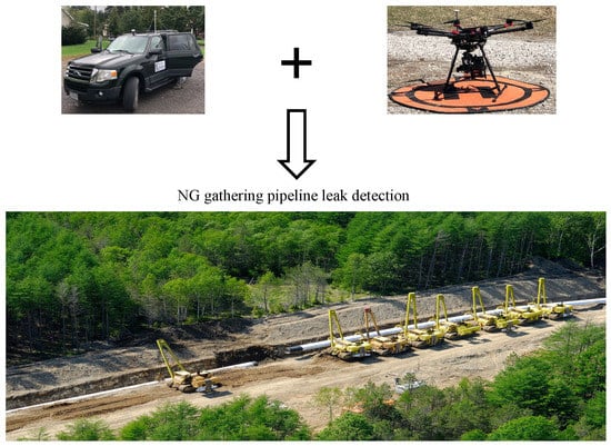
2. Methods
2.1. Access to Pipeline Location Data
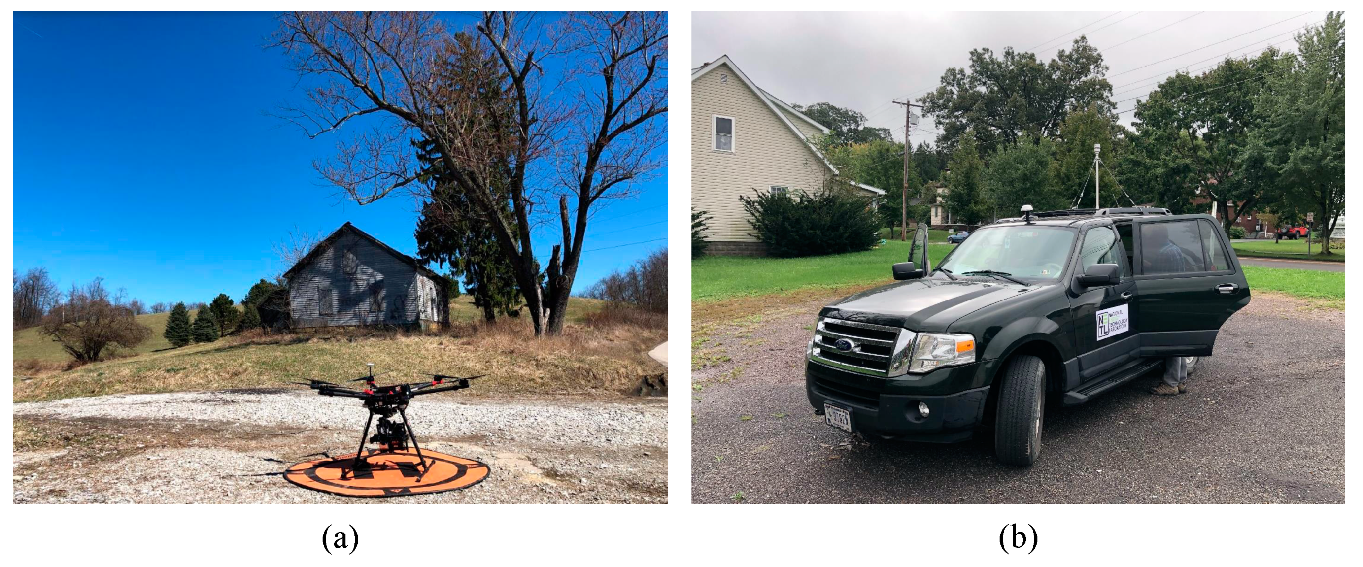
2.2. UAV Setup and Flight Plan
2.3. Ground-Based Vehicle Sampling Setup
2.4. Data Quality Control
2.5. Gaussian Dispersion Modeling
2.6. Controlled Release Experiment
3. Results and Discussion
3.1. TDLAS Minimum Detection Limit (MDL)
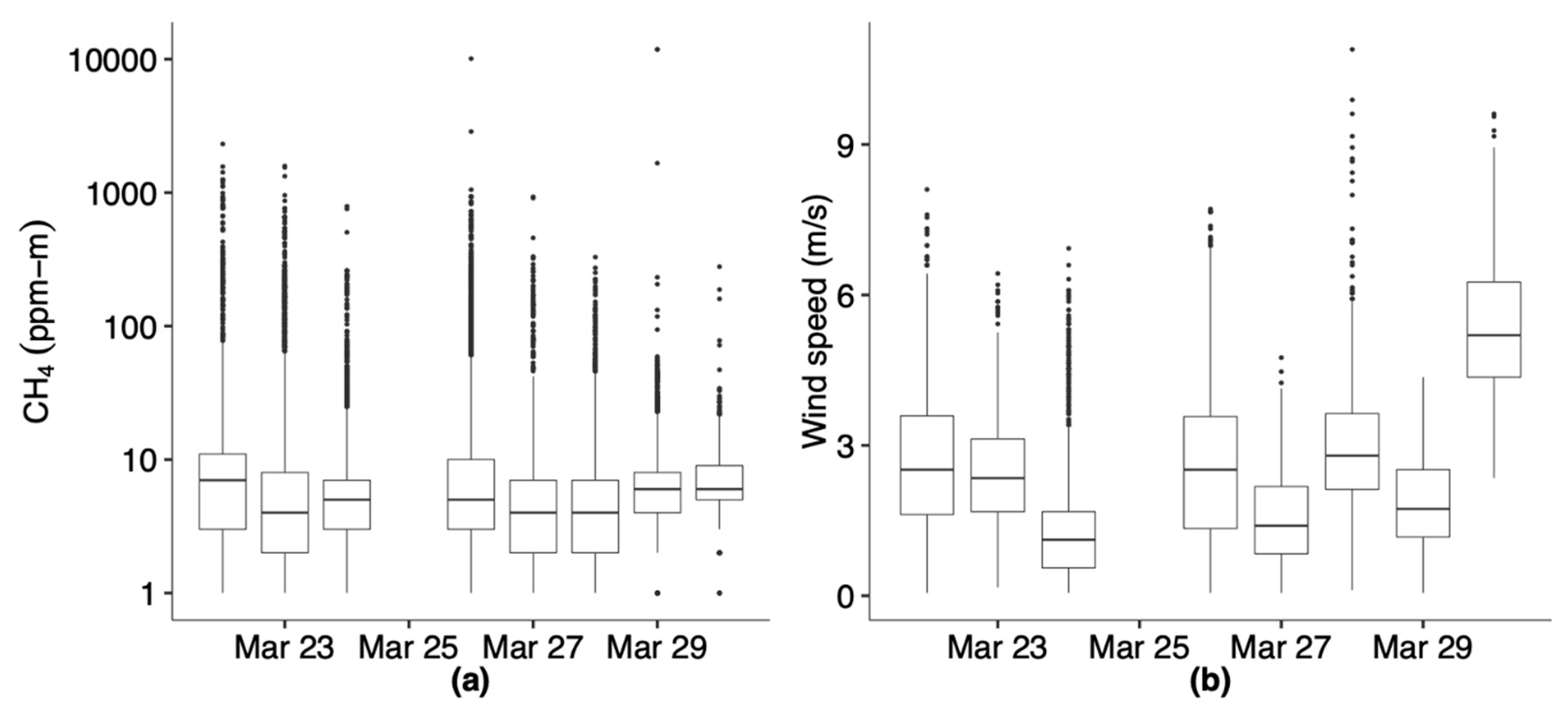
3.2. Low Pipeline Leak Frequency
4. Conclusions
Supplementary Materials
Author Contributions
Funding
Acknowledgments
Conflicts of Interest
References
- IPCC. Anthropogenic and Natural Radiative Forcing. In Climate Change 2013—The Physical Science Basis: Working Group I Contribution to the Fifth Assessment Report of the Intergovernmental Panel on Climate Change; Cambridge University Press: Cambridge, UK, 2014; pp. 659–740. ISBN 978-1-107-05799-9. [Google Scholar]
- US EPA Inventory of U.S. Greenhouse Gas Emissions and Sinks. Available online: https://www.epa.gov/ghgemissions/inventory-us-greenhouse-gas-emissions-and-sinks (accessed on 12 February 2019).
- EIA. EIA Carbon Dioxide Emissions Coefficients. Available online: https://www.eia.gov/environment/emissions/co2_vol_mass.php (accessed on 12 February 2019).
- EIA U.S. Dry Natural Gas Production (Million Cubic Feet). Available online: https://www.eia.gov/dnav/ng/hist/n9070us2A.htm (accessed on 3 July 2019).
- EIA. EIA Annual Energy Outlook. Available online: https://www.eia.gov/outlooks/aeo/ (accessed on 11 January 2019).
- EIA Natural Gas Imports and Exports—Energy Explained, Your Guide to Understanding Energy—Energy Information Administration. Available online: https://www.eia.gov/energyexplained/index.php?page=natural_gas_imports (accessed on 3 July 2019).
- Voulgarakis, A.; Naik, V.; Lamarque, J.-F.; Shindell, D.T.; Young, P.J.; Prather, M.J.; Wild, O.; Field, R.D.; Bergmann, D.; Cameron-Smith, P.; et al. Analysis of present day and future OH and methane lifetime in the ACCMIP simulations. Atmos. Chem. Phys. 2013, 13, 2563–2587. [Google Scholar] [CrossRef]
- Alvarez, R.A.; Pacala, S.W.; Winebrake, J.J.; Chameides, W.L.; Hamburg, S.P. Greater focus needed on methane leakage from natural gas infrastructure. Proc. Natl. Acad. Sci. USA 2012, 109, 6435–6440. [Google Scholar] [CrossRef] [PubMed]
- UNFCCC. The Paris Agreement|UNFCCC. Available online: https://unfccc.int/process-and-meetings/the-paris-agreement/the-paris-agreement (accessed on 24 June 2020).
- Alvarez, R.A.; Zavala-Araiza, D.; Lyon, D.R.; Allen, D.T.; Barkley, Z.R.; Brandt, A.R.; Davis, K.J.; Herndon, S.C.; Jacob, D.J.; Karion, A.; et al. Assessment of methane emissions from the U.S. oil and gas supply chain. Science 2018, eaar7204. [Google Scholar] [CrossRef] [PubMed]
- Campbell, L.M.; Campbell, M.V.; Epperson, D.L. Methane Emissions from the Natural Gas Industry. Undergr. Pipelines 1996, 9, 100. [Google Scholar]
- Zimmerle, D.J.; Pickering, C.K.; Bell, C.S.; Heath, G.A.; Nummedal, D.; Pétron, G.; Vaughn, T.L. Gathering pipeline methane emissions in Fayetteville shale pipelines and scoping guidelines for future pipeline measurement campaigns. Elem. Sci. Anthr. 2017, 5, 70. [Google Scholar] [CrossRef]
- PHMSA. Pipeline Incident 20 Year Trends. Available online: https://www.phmsa.dot.gov/data-and-statistics/pipeline/pipeline-incident-20-year-trends (accessed on 29 January 2019).
- Mitchell, A.L.; Tkacik, D.S.; Roscioli, J.R.; Herndon, S.C.; Yacovitch, T.I.; Martinez, D.M.; Vaughn, T.L.; Williams, L.L.; Sullivan, M.R.; Floerchinger, C.; et al. Measurements of Methane Emissions from Natural Gas Gathering Facilities and Processing Plants: Measurement Results. Environ. Sci. Technol. 2015, 49, 3219–3227. [Google Scholar] [CrossRef]
- Luck, B.; Zimmerle, D.; Vaughn, T.; Lauderdale, T.; Keen, K.; Harrison, M.; Marchese, A.J.; Williams, L.L.; Allen, D.T. Multi-day Measurements of Pneumatic Controller Emissions Reveal Frequency of Abnormal Emissions Behavior at Natural Gas Gathering Stations. Environ. Sci. Technol. Lett. 2019. [Google Scholar] [CrossRef]
- Subramanian, R.; Williams, L.L.; Vaughn, T.L.; Zimmerle, D.; Roscioli, J.R.; Herndon, S.C.; Yacovitch, T.I.; Floerchinger, C.; Tkacik, D.S.; Mitchell, A.L.; et al. Methane Emissions from Natural Gas Compressor Stations in the Transmission and Storage Sector: Measurements and Comparisons with the EPA Greenhouse Gas Reporting Program Protocol. Environ. Sci. Technol. 2015, 49, 3252–3261. [Google Scholar] [CrossRef]
- Li, H.Z.; Reeder, M.D.; Litten, J.; Pekney, N.J. Identifying under-characterized atmospheric methane emission sources in Western Maryland. Atmos. Environ. 2019, 117053. [Google Scholar] [CrossRef]
- Li, H.Z.; Dallmann, T.R.; Li, X.; Gu, P.; Presto, A.A. Urban Organic Aerosol Exposure: Spatial Variations in Composition and Source Impacts. Environ. Sci. Technol. 2017. [Google Scholar] [CrossRef]
- Omara, M.; Zimmerman, N.; Sullivan, M.R.; Li, X.; Ellis, A.; Cesa, R.; Subramanian, R.; Presto, A.A.; Robinson, A.L. Methane Emissions from Natural Gas Production Sites in the United States: Data Synthesis and National Estimate. Environ. Sci. Technol. 2018, 52, 12915–12925. [Google Scholar] [CrossRef] [PubMed]
- Omara, M.; Sullivan, M.R.; Li, X.; Subramanian, R.; Robinson, A.L.; Presto, A.A. Methane Emissions from Conventional and Unconventional Natural Gas Production Sites in the Marcellus Shale Basin. Environ. Sci. Technol. 2016, 50, 2099–2107. [Google Scholar] [CrossRef] [PubMed]
- von Fischer, J.C.; Cooley, D.; Chamberlain, S.; Gaylord, A.; Griebenow, C.J.; Hamburg, S.P.; Salo, J.; Schumacher, R.; Theobald, D.; Ham, J. Rapid, Vehicle-Based Identification of Location and Magnitude of Urban Natural Gas Pipeline Leaks. Environ. Sci. Technol. 2017, 51, 4091–4099. [Google Scholar] [CrossRef] [PubMed]
- Ye, Q.; Gu, P.; Li, H.Z.; Robinson, E.S.; Lipsky, E.; Kaltsonoudis, C.; Lee, A.K.Y.; Apte, J.S.; Robinson, A.L.; Sullivan, R.C.; et al. Spatial Variability of Sources and Mixing State of Atmospheric Particles in a Metropolitan Area. Environ. Sci. Technol. 2018, 52, 6807–6815. [Google Scholar] [CrossRef]
- Ren, X.; Salmon, O.E.; Hansford, J.R.; Ahn, D.; Hall, D.; Benish, S.E.; Stratton, P.R.; He, H.; Sahu, S.; Grimes, C.; et al. Methane Emissions From the Baltimore-Washington Area Based on Airborne Observations: Comparison to Emissions Inventories. J. Geophys. Res. Atmos. 2018, 123, 8869–8882. [Google Scholar] [CrossRef]
- Cui, Y.Y.; Henze, D.K.; Brioude, J.; Angevine, W.M.; Liu, Z.; Bousserez, N.; Guerrette, J.; McKeen, S.A.; Peischl, J.; Yuan, B.; et al. Inversion Estimates of Lognormally Distributed Methane Emission Rates From the Haynesville-Bossier Oil and Gas Production Region Using Airborne Measurements. J. Geophys. Res. Atmos. 2019, 124, 3520–3531. [Google Scholar] [CrossRef]
- Vaughn, T.L.; Bell, C.S.; Pickering, C.K.; Schwietzke, S.; Heath, G.A.; Pétron, G.; Zimmerle, D.J.; Schnell, R.C.; Nummedal, D. Temporal variability largely explains top-down/bottom-up difference in methane emission estimates from a natural gas production region. Proc. Natl. Acad. Sci. USA 2018, 115, 11712–11717. [Google Scholar] [CrossRef]
- Yang, S.; Talbot, R.; Frish, M.; Golston, L.; Aubut, N.; Zondlo, M.; Gretencord, C.; McSpiritt, J. Natural Gas Fugitive Leak Detection Using an Unmanned Aerial Vehicle: Measurement System Description and Mass Balance Approach. Atmosphere 2018, 9, 383. [Google Scholar] [CrossRef]
- Golston, L.; Aubut, N.; Frish, M.; Yang, S.; Talbot, R.; Gretencord, C.; McSpiritt, J.; Zondlo, M. Natural Gas Fugitive Leak Detection Using an Unmanned Aerial Vehicle: Localization and Quantification of Emission Rate. Atmosphere 2018, 9, 333. [Google Scholar] [CrossRef]
- Barbieri, L.; Kral, S.; Bailey, S.; Frazier, A.; Jacob, J.; Reuder, J.; Brus, D.; Chilson, P.; Crick, C.; Detweiler, C.; et al. Intercomparison of Small Unmanned Aircraft System (sUAS) Measurements for Atmospheric Science during the LAPSE-RATE Campaign. Sensors 2019, 19, 2179. [Google Scholar] [CrossRef]
- Lee, T.; Buban, M.; Dumas, E.; Baker, C. On the Use of Rotary-Wing Aircraft to Sample Near-Surface Thermodynamic Fields: Results from Recent Field Campaigns. Sensors 2018, 19, 10. [Google Scholar] [CrossRef] [PubMed]
- Nolan, P.; McClelland, H.; Woolsey, C.; Ross, S. A Method for Detecting Atmospheric Lagrangian Coherent Structures Using a Single Fixed-Wing Unmanned Aircraft System. Sensors 2019, 19, 1607. [Google Scholar] [CrossRef] [PubMed]
- Rautenberg, A.; Graf, M.; Wildmann, N.; Platis, A.; Bange, J. Reviewing Wind Measurement Approaches for Fixed-Wing Unmanned Aircraft. Atmosphere 2018, 9, 422. [Google Scholar] [CrossRef]
- Rautenberg, A.; Schön, M.; Zum Berge, K.; Mauz, M.; Manz, P.; Platis, A.; van Kesteren, B.; Suomi, I.; Kral, S.T.; Bange, J. The Multi-Purpose Airborne Sensor Carrier MASC-3 for Wind and Turbulence Measurements in the Atmospheric Boundary Layer. Sensors 2019, 19, 2292. [Google Scholar] [CrossRef]
- Schuyler, T.; Guzman, M. Unmanned Aerial Systems for Monitoring Trace Tropospheric Gases. Atmosphere 2017, 8, 206. [Google Scholar] [CrossRef]
- Schuyler, T.J.; Bailey, S.C.C.; Guzman, M.I. Monitoring Tropospheric Gases with Small Unmanned Aerial Systems (sUAS) during the Second CLOUDMAP Flight Campaign. Atmosphere 2019, 10, 434. [Google Scholar] [CrossRef]
- Schuyler, T.J.; Gohari, S.M.I.; Pundsack, G.; Berchoff, D.; Guzman, M.I. Using a Balloon-Launched Unmanned Glider to Validate Real-Time WRF Modeling. Sensors 2019, 19, 1914. [Google Scholar] [CrossRef]
- Witte, B.; Singler, R.; Bailey, S. Development of an Unmanned Aerial Vehicle for the Measurement of Turbulence in the Atmospheric Boundary Layer. Atmosphere 2017, 8, 195. [Google Scholar] [CrossRef]
- Gu, P.; Li, H.Z.; Ye, Q.; Robinson, E.S.; Apte, J.S.; Robinson, A.L.; Presto, A.A. Intracity Variability of Particulate Matter Exposure Is Driven by Carbonaceous Sources and Correlated with Land-Use Variables. Environ. Sci. Technol. 2018, 52, 11545–11554. [Google Scholar] [CrossRef]
- Li, H.Z.; Gu, P.; Ye, Q.; Zimmerman, N.; Robinson, E.S.; Subramanian, R.; Apte, J.S.; Robinson, A.L.; Presto, A.A. Spatially dense air pollutant sampling: Implications of spatial variability on the representativeness of stationary air pollutant monitors. Atmos. Environ. X 2019, 100012. [Google Scholar] [CrossRef]
- Li, H.Z.; Dallmann, T.R.; Gu, P.; Presto, A.A. Application of mobile sampling to investigate spatial variation in fine particle composition. Atmos. Environ. 2016, 142, 71–82. [Google Scholar] [CrossRef]
- Robinson, E.S.; Gu, P.; Ye, Q.; Li, H.Z.; Shah, R.U.; Apte, J.S.; Robinson, A.L.; Presto, A.A. Restaurant Impacts on Outdoor Air Quality: Elevated Organic Aerosol Mass from Restaurant Cooking with Neighborhood-Scale Plume Extents. Environ. Sci. Technol. 2018. [Google Scholar] [CrossRef]
- Phillips, N.G.; Ackley, R.; Crosson, E.R.; Down, A.; Hutyra, L.R.; Brondfield, M.; Karr, J.D.; Zhao, K.; Jackson, R.B. Mapping urban pipeline leaks: Methane leaks across Boston. Environ. Pollut. 2013, 173, 1–4. [Google Scholar] [CrossRef] [PubMed]
- Saha, P.K.; Zimmerman, N.; Malings, C.; Hauryliuk, A.; Li, Z.; Snell, L.; Subramanian, R.; Lipsky, E.; Apte, J.S.; Robinson, A.L.; et al. Quantifying high-resolution spatial variations and local source impacts of urban ultrafine particle concentrations. Sci. Total Environ. 2019, 655, 473–481. [Google Scholar] [CrossRef] [PubMed]
- Connolly, J.I.; Robinson, R.A.; Gardiner, T.D. Assessment of the Bacharach Hi Flow® Sampler characteristics and potential failure modes when measuring methane emissions. Measurement 2019, 145, 226–233. [Google Scholar] [CrossRef]
- McGill, R.; Tukey, J.W.; Larsen, W.A. Variations of Box Plots. Am. Stat. 1978, 32, 12. [Google Scholar] [CrossRef]
- Atherton, E.; Risk, D.; Fougère, C.; Lavoie, M.; Marshall, A.; Werring, J.; Williams, J.P.; Minions, C. Mobile measurement of methane emissions from natural gas developments in northeastern British Columbia, Canada. Atmos. Chem. Phys. 2017, 17, 12405–12420. [Google Scholar] [CrossRef]
- Turner, D.B. Workbook of Atmospheric Dispersion Estimates: An Introduction to Dispersion Modeling, Second Edition; CRC Press: Boca Raton, FL, USA, 1994; ISBN 978-1-56670-023-8. [Google Scholar]
- Lamb, B.K.; Edburg, S.L.; Ferrara, T.W.; Howard, T.; Harrison, M.R.; Kolb, C.E.; Townsend-Small, A.; Dyck, W.; Possolo, A.; Whetstone, J.R. Direct Measurements Show Decreasing Methane Emissions from Natural Gas Local Distribution Systems in the United States. Environ. Sci. Technol. 2015, 49, 5161–5169. [Google Scholar] [CrossRef]
- Caulton, D.R.; Li, Q.; Bou-Zeid, E.; Fitts, J.P.; Golston, L.M.; Pan, D.; Lu, J.; Lane, H.M.; Buchholz, B.; Guo, X.; et al. Quantifying uncertainties from mobile-laboratory-derived emissions of well pads using inverse Gaussian methods. Atmos. Chem. Phys. 2018, 18, 15145–15168. [Google Scholar] [CrossRef]
- AOGC. 2018 Arkansas Production & Well Data. Available online: http://www.aogc2.state.ar.us/welldata/default.aspx (accessed on 5 July 2019).
- Ohio DNR Ohio Oil & Gas Well Production Numbers. Available online: http://oilandgas.ohiodnr.gov/production#COMB (accessed on 5 July 2019).
- Ulrich, B.A.; Mitton, M.; Lachenmeyer, E.; Hecobian, A.; Zimmerle, D.; Smits, K.M. Natural Gas Emissions from Underground Pipelines and Implications for Leak Detection. Environ. Sci. Technol. Lett. 2019. [Google Scholar] [CrossRef]
- Nolan, P.; Pinto, J.; González-Rocha, J.; Jensen, A.; Vezzi, C.; Bailey, S.; de Boer, G.; Diehl, C.; Laurence, R.; Powers, C.; et al. Coordinated Unmanned Aircraft System (UAS) and Ground-Based Weather Measurements to Predict Lagrangian Coherent Structures (LCSs). Sensors 2018, 18, 4448. [Google Scholar] [CrossRef] [PubMed]
- Alaoui-Sosse, S.; Durand, P.; Medina, P.; Pastor, P.; Lothon, M.; Cernov, I. OVLI-TA: An Unmanned Aerial System for Measuring Profiles and Turbulence in the Atmospheric Boundary Layer. Sensors 2019, 19, 581. [Google Scholar] [CrossRef] [PubMed]
- Li, H.Z.; Reeder, M.D.; Pekney, N.J. Quantifying source contributions of volatile organic compounds under hydraulic fracking moratorium. Sci. Total Environ. 2020, 139322. [Google Scholar] [CrossRef] [PubMed]
- Gu, P.; Dallmann, T.R.; Li, H.Z.; Tan, Y.; Presto, A.A. Quantifying Urban Spatial Variations of Anthropogenic VOC Concentrations and Source Contributions with a Mobile Sampling Platform. Int. J. Environ. Res. Public. Health 2019, 16, 1632. [Google Scholar] [CrossRef]
- Shah, R.U.; Coggon, M.M.; Gkatzelis, G.I.; McDonald, B.C.; Tasoglou, A.; Huber, H.; Gilman, J.; Warneke, C.; Robinson, A.L.; Presto, A.A. Urban Oxidation Flow Reactor Measurements Reveal Significant Secondary Organic Aerosol Contributions from Volatile Emissions of Emerging Importance. Environ. Sci. Technol. 2020, acs.est.9b06531. [Google Scholar] [CrossRef] [PubMed]
- Ye, Q.; Li, H.Z.; Gu, P.; Robinson, E.S.; Apte, J.S.; Sullivan, R.C.; Robinson, A.L.; Donahue, N.M.; Presto, A.A. Moving beyond Fine Particle Mass: High-Spatial Resolution Exposure to Source-Resolved Atmospheric Particle Number and Chemical Mixing State. Environ. Health Perspect. 2020, 128, 017009. [Google Scholar] [CrossRef]
- Donahue, N.M.; Posner, L.N.; Westervelt, D.M.; Li, Z.; Shrivastava, M.; Presto, A.A.; Sullivan, R.C.; Adams, P.J.; Pandis, S.N.; Robinson, A.L. Where Did This Particle Come From? Sources of Particle Number and Mass for Human Exposure Estimates. In Issues in Environmental Science and Technology; Harrison, R.M., Hester, R.E., Querol, X., Eds.; Royal Society of Chemistry: Cambridge, UK, 2016; pp. 35–71. ISBN 978-1-78262-491-2. [Google Scholar]
- Robinson, E.S.; Shah, R.U.; Messier, K.; Gu, P.; Li, H.Z.; Apte, J.S.; Robinson, A.L.; Presto, A.A. Land-Use Regression Modeling of Source-Resolved Fine Particulate Matter Components from Mobile Sampling. Environ. Sci. Technol. 2019, 53, 8925–8937. [Google Scholar] [CrossRef]


| Date | Number of Flights | Weather | Distance Flown (km) |
|---|---|---|---|
| 3/22/2019 | 4 | Morning scattered rain with high winds in the afternoon | 2.3 |
| 3/23/2019 | 9 | Mostly sunny | 5.1 |
| 3/24/2019 | 9 | Mostly sunny | 7.2 |
| 3/25/2019 | 0 | Rain all day | 0 |
| 3/26/2019 | 8 | Sunny | 7.4 |
| 3/27/2019 | 8 | Sunny | 10 |
| 3/28/2019 | 8 | Partly cloudy | 9.6 |
| 3/29/2019 | 5 | Overcast, light winds | 11.7 |
| 3/30/2019 | 2 | Strong winds | 2.3 |
© 2020 by the authors. Licensee MDPI, Basel, Switzerland. This article is an open access article distributed under the terms and conditions of the Creative Commons Attribution (CC BY) license (http://creativecommons.org/licenses/by/4.0/).
Share and Cite
Li, H.Z.; Mundia-Howe, M.; Reeder, M.D.; Pekney, N.J. Gathering Pipeline Methane Emissions in Utica Shale Using an Unmanned Aerial Vehicle and Ground-Based Mobile Sampling. Atmosphere 2020, 11, 716. https://doi.org/10.3390/atmos11070716
Li HZ, Mundia-Howe M, Reeder MD, Pekney NJ. Gathering Pipeline Methane Emissions in Utica Shale Using an Unmanned Aerial Vehicle and Ground-Based Mobile Sampling. Atmosphere. 2020; 11(7):716. https://doi.org/10.3390/atmos11070716
Chicago/Turabian StyleLi, Hugh Z., Mumbi Mundia-Howe, Matthew D. Reeder, and Natalie J. Pekney. 2020. "Gathering Pipeline Methane Emissions in Utica Shale Using an Unmanned Aerial Vehicle and Ground-Based Mobile Sampling" Atmosphere 11, no. 7: 716. https://doi.org/10.3390/atmos11070716
APA StyleLi, H. Z., Mundia-Howe, M., Reeder, M. D., & Pekney, N. J. (2020). Gathering Pipeline Methane Emissions in Utica Shale Using an Unmanned Aerial Vehicle and Ground-Based Mobile Sampling. Atmosphere, 11(7), 716. https://doi.org/10.3390/atmos11070716