Article

Objective Identification and Multi-Scale Controlling Factors of Extreme Heat-Wave Events in Southern China

1
Department of Atmospheric & Oceanic Sciences and Institute of Atmospheric Sciences, Fudan University, Shanghai 200438, China
2
School of Atmospheric Sciences, Chengdu University of Information Technology, Chengdu 610225, China
3
Innovation Center of Ocean and Atmosphere System, Zhuhai Fudan Innovation Research Institute, Zhuhai 518057, China
*
Author to whom correspondence should be addressed.
Atmosphere 2020, 11(6), 668; https://doi.org/10.3390/atmos11060668
Submission received: 1 May 2020 / Revised: 17 June 2020 / Accepted: 19 June 2020 / Published: 23 June 2020

Abstract

:
Southern China (SC) is often subjected to the impacts of extreme heat-wave (EHW) events with hot days covering large areas and lasting extended periods in the boreal summer. The present study explores new objective identification methods of the EHW events and reveals the controlling factors of different spatial-temporal variations in shaping the EHW events over SC from 2000 to 2017 with in-situ observations and latest reanalysis. A compound index of the EHW (with impact area, duration, and magnitude) was defined to quantify the overall intensity of the EHW events in SC. It was found that synoptic variability and 10–30-day intra-seasonal variability (ISV) induce the onsets of the EHW events, while 30–90-day ISV shapes the durations. An innovative daily compound index was introduced to track the outbreak of the EHW events. The occurrences of the EHW in SC are coincident with the arrivals of intra-seasonal signals (e.g., the anomalies of outgoing long-wave radiation (OLR) and 500 hPa geopotential height) propagating from the east and south. About 12 days before the onset of the EHW in SC, the 10–30-day positive anomalies of 500 hPa geopotential height and OLR appear near the equatorial western Pacific, which then propagate northwestward to initiate the EHW in SC. At the same time, the 30–90-day suppressed phase propagates northeastward from the Indian Ocean to the SC to sustain the EHW events. On the interannual time scale, it was found that the EHW events in SC occurred in those years with robust warming of the western North Pacific in early summer (May and June) and warming of the equatorial eastern Pacific in the preceding winter (December, January, and February). An interannual sea surface temperature anomalous (SSTA) index, which adds together the SSTA over the above two regions, serves as a very useful seasonal predictor for the EHW occurrences in SC at least one-month ahead.

1. Introduction

A recent World Meteorological Organization report [1] has clearly shown that, in association with global warming, the occurrences of extreme meteorological events have increased steadily in past decades. These extreme events have caused tremendous economic and societal losses around the world and are threatening the sustainable development of global society. To better understand the processes controlling these extreme events and to develop advanced prediction capability for these extremes are forefront grand challenges faced by the global meteorological community.
In China, the frequent occurrences of large-scale events with air temperature exceeding 35 °C and the resulting disasters have drawn great attention of governments and the meteorological community [2,3]. Heat-waves, which have occurred in many places of China, with such high air temperature, widespread extent, and prolonged duration are extremely harmful,. For example, in the 2003 summer, a severe heat-wave occurred over a large area from the south of the Yangtze River to the middle of Southern China (SC), which caused tremendous stresses on the local transportation, water, electricity and other urban operational lifelines as well as societal and economic activities [2]. For such a heat-wave event, the days with maximum air temperature exceeding 38 °C are 5–20-days more than the climatology. In the 2013 summer, another severe heat-wave hit the Yangtze River Basin of China, resulting in direct economic loss amounting to 59 billion Chinese Yuan [3].
Unlike visible, destructive and violent extreme meteorological events (e.g., floods, tropical cyclones and tornadoes etc.), the Extreme-Heat-Wave (EHW) events exert great threats to society and human health in an unconscious way, thus gaining the nickname of “silent killer”. Due to the complex multi-scale processes involved in the making of extreme meteorological events [2,4,5,6,7] and the chaotic nature of the atmosphere, it is very difficult to predict the extreme events accurately with sufficient lead times, which brings many restrictions to effective disaster prevention and reduction [1]. Therefore, it is of great scientific and societal implication to better understand the controlling factors and predictability of the EHW. Many previous studies have investigated the respective impacts of synoptic weather systems, subseasonal-to-seasonal, and interannual-to-decadal variations on the heat-wave.
On the synoptic time scale, Ding and Qian [2] pointed out that the synoptic precursors of the heat-wave in China can be found from the 250 hPa continent-scale geopotential height anomalies, which move westward in low latitudes and east-southeastward in middle latitudes; for SC, the precursors from the northwest Pacific have an averaged lead time of 4.6 days, the precursors initiated over Europe and northwest China have lead times ranging from 2 to 15 days. Wang et al. [4] found that East-Asian EHW events are strongly associated with the “exit” and the “tail” regions of the East-Asian jet stream. Poleward displacement of the jet-exit region is associated with warming tropospheric air temperatures over East Asia and tends to be linked with high EHW frequency, while enhancement of the tail is associated with cooling tropospheric air temperatures in the northern Pacific and tends to be linked with low EHW frequency. Li et al. [8] attributed the 2013 summer heat-wave to a result of the westward extensions of the stable and strong western Pacific subtropical high. In this summer, there were four westward pulses of western Pacific subtropical high, which directly led to four heat-wave periods over the SC. Wang et al. [9] pointed out that the coupling between the westward-enhanced western Pacific subtropical high and the poleward-displaced East-Asian jet stream blocked the moisture supply from the southwest monsoon, resulting in the eastern China heat-wave in 2013. Chen et al. [10] found that when the atmosphere is in a quasi-barotropic state, it is easier to form widespread persistent high air temperature weather systems. Loikith and Broccoli [11] showed that warm extremes at most locations in North America are associated with wavy patterns: Positive 500 hPa geopotential height and sea level pressure anomalies in the downstream along with negative anomalies farther upstream.
On subseasonal-to-seasonal time scales, Chen et al. [5] pointed out that the daily air temperature and circulation anomalies over the SC exhibit fluctuations with a period of about 10 days, largely resulting from the influence of quasi-biweekly oscillation, which originates from the tropical western Pacific and propagates northwestward. The biweekly oscillation explains more than 50% of the 5–25-day variance of daily maximum air temperature and vorticity over SC and 80% of heat-wave onset timing. Gao et al. [12] found that when a significantly low-level anticyclonic anomaly associated with biweekly oscillation appears over the Yangtze River valley, air temperature rises sharply due to the adiabatic heating associated with subsidence and the enhanced downward solar radiation associated with reduced clouds. Diao et al. [13] pointed out that when the positive rainfall anomaly of the boreal-summer intraseasonal oscillation is primarily located over a northwest–southeast-oriented belt extending from India to Maritime Continent and a negative rainfall anomalous belt exists in southeast Asia and western North Pacific, the occurrence probability of EHW events in the Asian-Pacific sector is significantly elevated. Chen et al. [6] found that the fluctuating anomalies of daily maximum air temperature over SC and the western Pacific are intimately related to two intraseasonal modes, namely, the 5–25-day and 30–90-day oscillations, which originate from the tropical western Pacific and propagate northwestward. The 5–25-day oscillation is vital in triggering and terminating the heat-wave, accounting for approximately 50% transitions of the daily air temperature and circulation anomalies in the raw time series. The 30–90-day oscillation favors the persistent warming during heat-wave events, accounting for approximately one-third of the prolonged warming and anticyclonic anomalies. Chen and Zhai [14] indicated that the boreal-summer intraseasonal oscillation can simultaneously facilitate precipitation extremes in central-eastern China and EHW events in southern and southeast China. It is the overturning circulation of the boreal-summer intraseasonal oscillation, with ascending motion in the Yangtze-Huai River Basin and descending motion in the south, that results in the simultaneous, but opposite extremes.
On interannual-to-decadal time scales, Ding et al. [15] indicated that, over most of China except northwestern China, the frequency of the heat-wave exhibits a high-low-high fluctuating pattern, respectively, for the 1960s–1970s, 1980s, and afterwards. A remarkable upward trend of the heat-wave exists after the 1990s over entire China. It is also found that the interannual-to-interdecadal variations of the heat-wave are closely related to the variations of rainy days and atmospheric circulation patterns. On the decadal time scale, Chen et al. [16] found that the relationships among the SC air temperature, large-scale atmospheric circulation pattern over the Eurasia and the tropical sea surface temperature anomaly (SSTA) experienced a decadal shift around the early 1990s. Before the early 1990s, the warmer summer in SC largely originated from teleconnection from high latitude, which is featured by higher pressure over the Ural Mountains and the Korean Peninsula and lower pressure around Lake Baikal. After the early 1990s, the SC air temperature is primarily influenced by the tropical SSTA with the impact of high-latitude teleconnection considerably weakened.
Most of the aforementioned literature focuses on the impacts of a given time-scale variability on the EHW events. In fact, severe extreme weather events usually result from compound (combined) influences from multiscale variability. For example, Song and Wu [17] investigated the strong cold events over eastern China in the boreal winter. They found that the intra-seasonal oscillations and synoptic systems, respectively, explain about 55% and 20% of the total area-mean air temperature anomaly in eastern China. For EHW events, our understanding on the roles of multi-scale variability is still very limited.
This study targets the EHW events in China and reveals the associated multi-scale impacting factors. Since most EHW events in China occurred in SC [18], this study will specifically focus on the EHW events occurred between 2000 and 2017 in SC. The questions that we will address in this study include: how to objectively identify the EHW events in SC? What are the major multi-scale factors controlling the occurrences, onsets, and lifecycles of the EHW events in SC?
The remaining parts of this article are organized as following. The data used in this study, selection criteria of a heat-wave and the definition of a compound EHW index are given in Section 2. Section 3 applies the methods given in Section 2 to select all heat-waves and identify the EHW events between 2000 and 2017 in SC as our research targets. Section 4 unravels the controlling factors of multi-scale variations on the lifecycles of 11 top EHW events. The concluding remarks and discussions are given in Section 5.

2. Data and Methodology
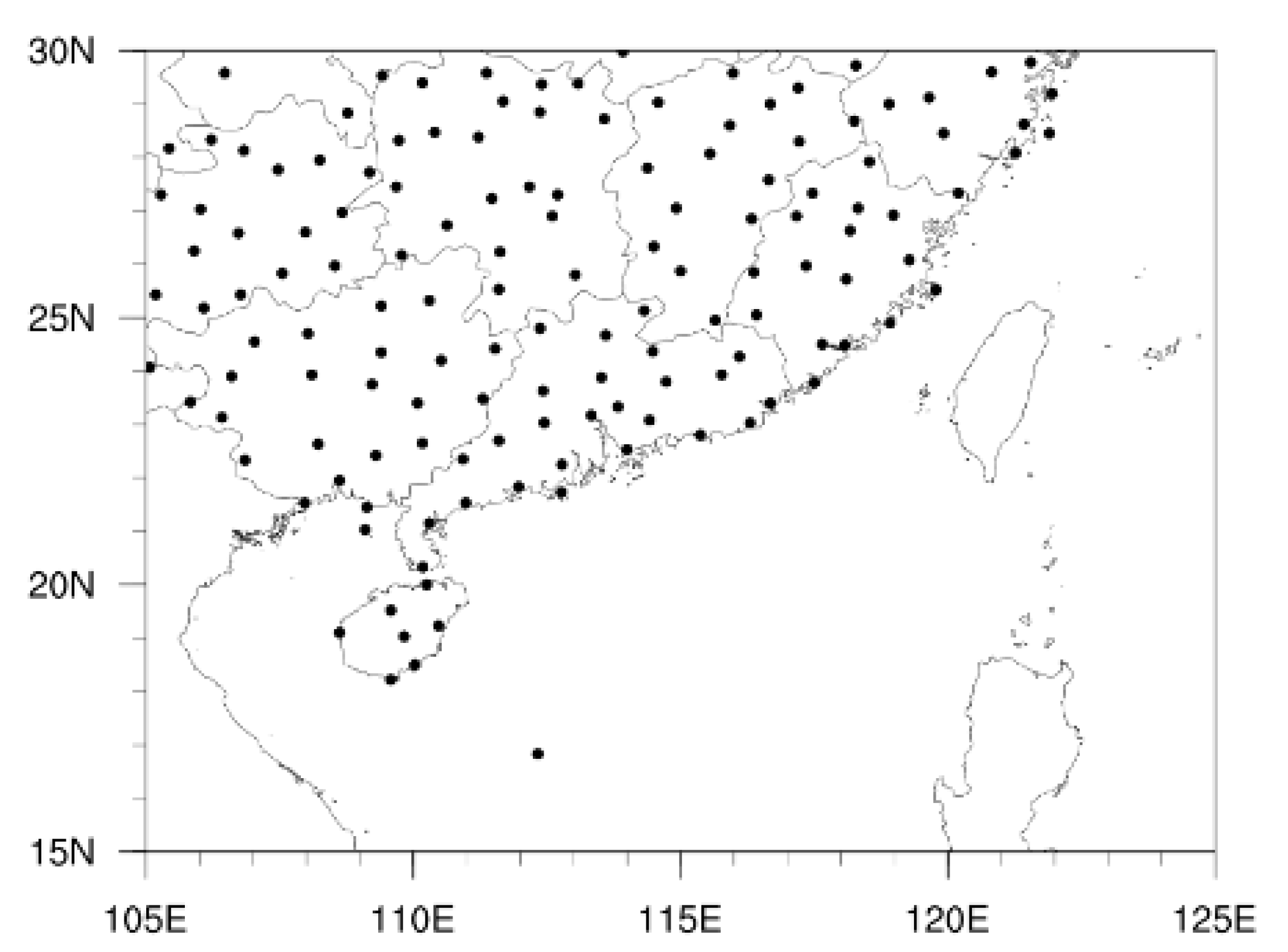
2.1. Data

The data used in this study include the daily measurements of basic meteorological stations in China, the ERA5 reanalysis, and outgoing longwave radiation (OLR). Station measurements include daily maximum air temperature. Among all the stations, 139 located in the domain of (15° N~30° N, 105° E~125° E) have been used to represent the SC (Chen et al. [5]). The spatial distribution of the 139 stations can be seen from Figure A1 in Appendix A. The ERA5 hourly reanalysis at a resolution of 0.25° × 0.25° is the latest reanalysis produced by the European Centre for Medium-Range Weather Forecasts (ECMWF) [19]. The variables of the ERA5 we used in this study include the zonal and meridional components of wind, geopotential height, 2 m air temperature, and sea surface temperature. The OLR daily mean data used in the study were acquired from the National Oceanic and Atmospheric Administration (NOAA), with a resolution of 2.5° × 2.5°. The ERA5 data were interpolated by mean onto a common horizontal resolution: 2.5° × 2.5°. All of these datasets span the 18 years from 2000 to 2017.

2.2. Method to Define Heat-Wave Events

In this study, the definition of heat-wave events basically follows Ding and Qian [18]. The impacts of heat-wave events not only depend on the instantaneous values of air temperature, but the daily maximum, as well as the duration and area covered. In order to define a compound heat-wave index to consider all the aforementioned factors, we first rank the daily maximum air temperatures of individual stations (139 in total) in SC from large to small in the 18 years to find out the threshold of the 90th percentile of each station (use all the daily values of the years). Then, we define an abnormal high air temperature day for each individual station if the daily maximum air temperature of the station exceeds the threshold of the 90th percentile.
Since the abnormal high air temperature of a given site need to last several days to have significant impact on human beings [18], the heat-wave events we targeted in this study were required to last at least one week. To be valid as a heat-wave event, its impact area should cover at least 10 adjacent stations in the same period [18]. The distance between any two stations, i and j, is estimated as:
D = [ lat ( i ) lat ( j ) ] 2 + [ lon ( i ) lon ( j ) ] 2 ,   i     j ,
where the lat(i) and lon(i) are the ith station’s latitude and longitude. If D ≤ 3, two stations were considered to be adjacent [18].
In summary, when there are more than 10 adjacent stations whose daily maximum air temperature exceeds its own threshold of 90th percentile and lasts for more than 7 days, this event is defined as a heat-wave event in SC. In addition, in order to facilitate the selection of events, if there is one day within the scope of definition that does not meet the requirements, it is determined as the end time of the event. In other words, the minimum interval between two events is one day.

2.3. Definition of Heat-Wave Compound Index

In several previous studies, there have been many works about the definition and identification of heat-wave events for other regions of the world [20,21,22,23]. For example, in the work of Stefanon et al. [20], they use a simple definition based on temperature only: a heat-wave event is defined when the temperature exceeds a given threshold, and they impose additional constraints on the spatial and temporal extensions. Researchers are generally aware that a heat-wave should be measured in terms of duration and extent of impact. However, the difference in heat intensity between different heat-wave events is ignored, which means that two events of the same length will be considered as equally severe, even if one of them has a higher air temperature values than the other. Therefore, there is a need to redefine a heat-wave index, which can account for the duration, impact extent, and intensity of the heat-wave. With such a compound index, the selected heat-wave events can be ranked quantitatively, which will facilitate the study of the controlling factors and the predictability of the most severe heat-wave events.
For all heat-wave events selected in Section 2.2, an integrated compound index is defined for individual heat-wave events based on their durations, the numbers of abnormal sites, and the degrees to which the daily maximum air temperature is higher than the threshold of the 90th percentile. The formula used to calculate the compound index of a given heat-wave event is the following:
C(i) = T(i) + A(i) + S(i),
The C(i) represents the compound index of the ith event. The T(i), A(i), and S(i), respectively, are the standardized duration index, area index and strength index by using the Z-score standardization [24]. The duration index T(i) is obtained by standardizing the duration of the ith event. The longer the event lasts, the greater the duration index. The area index A(i) reflects the spatial impact of the ith event, which is calculated by standardizing the number of abnormal stations whose daily maximum air temperature exceeds the threshold of the 90th percentile between the beginning and the end of the event. The larger the number of abnormal sites during the event, the wider the impact scope of the event and the larger the value of the area index. In order to avoid events with similar duration index and area index but larger difference in daily maximum air temperature being mistaken for an event of the same degree, the calculation method of the strength index S(i) is as follows: first, calculating the sum of the deviation between the daily maximum air temperature of each station and 35 °C for the ith event (including several days and stations), then averaging the sum for the number of days and stations, and finally standardizing. The larger the strength index, the stronger is this event.

3. The Objective Identification of the EHW Events

According to the definition of heat-wave events in Section 2.2, all the heat-wave events in SC from 2000 to 2017 were selected. During this period, there were 43 heat-wave events occurring in SC. Among these heat-wave events, the durations of some events can be as long as 30 days, the others can be as short as 7 days. The number of stations with abnormal high air temperature varies between 129 and 10. On average, there are 2.4 heat-wave events annually. During this period, each year has at least one heat-wave event, with a maximum of three events in some years. Among the 43 heat-wave events, there are eight events lasting more than 15 days (including 15 days); the others last less than 15 days. The events lasting more than 15 days occurred once, respectively, in 2003, 2007, 2013, 2014, 2016 and 2017, but twice in 2010 (Table A1 in Appendix A).
The compound indices of 43 selected heat-wave events are calculated. Their values vary between a maximum of 7.22 and a minimum of −4.02. The negative values indicate that the overall intensities of these events are below the median strength of all selected events. All events with a compound index smaller than one are categorized as normal. In this study, we simply lumped all events with the compound index larger than one as EHW events. Among all the 43 heat-wave events, there are 11 heat-wave events with a compound index greater than 1.0 (Table 1), which will serve as the target EHW events in this study. Among these top 11 EHW events, there are six events that last longer than 15 days and five events that last less than 15 days. Ten of 11 EHW events have their onset days in July. The two most severe EHW events occurred, respectively, in 2003 and 2013. These two ultra-extreme cases lasted much longer than 15 days and have drawn much attention and been widely studied as mentioned in introduction [2,3].

4. The Multi-Scale Controlling Factors of the EHW Events

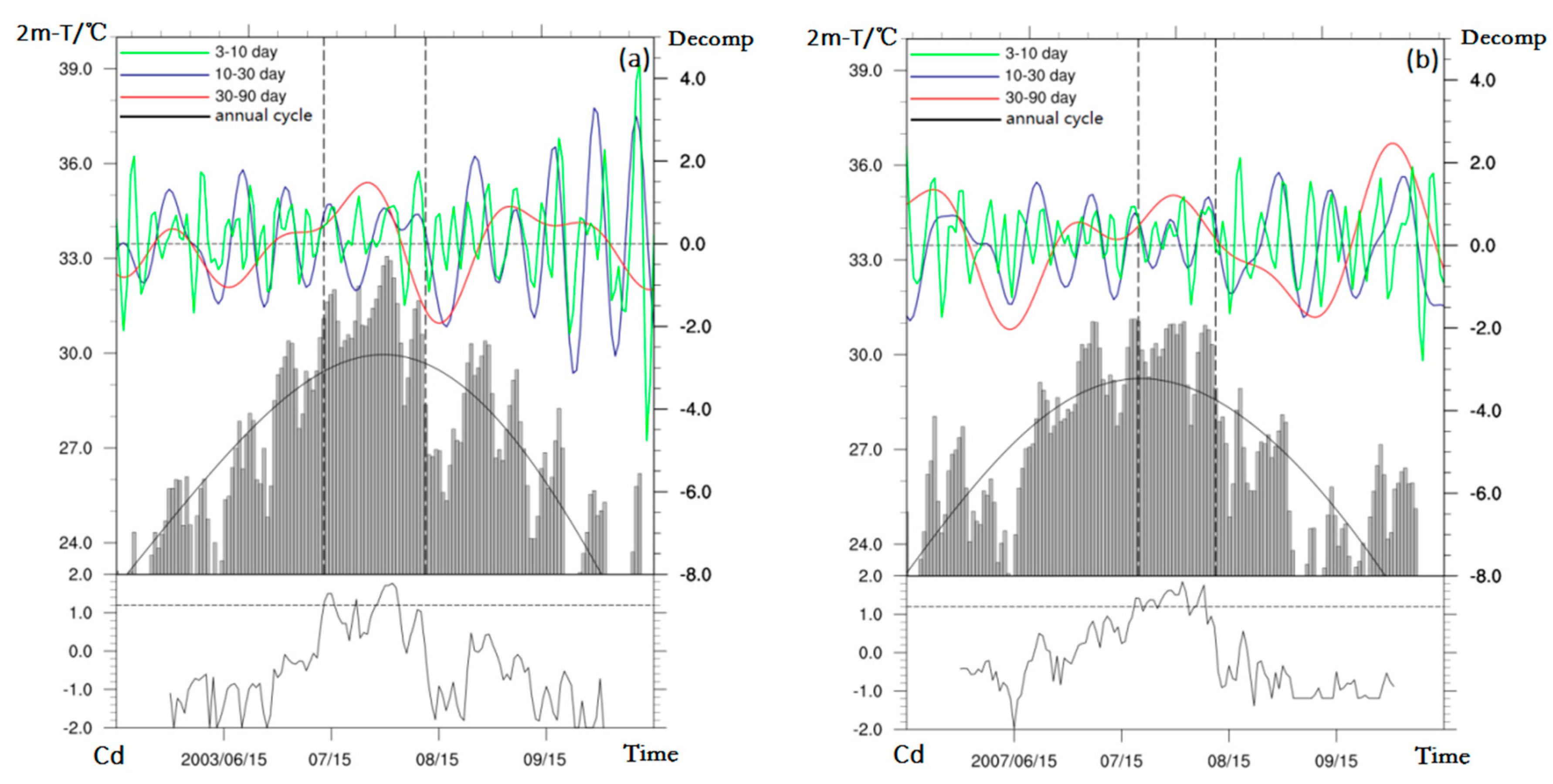
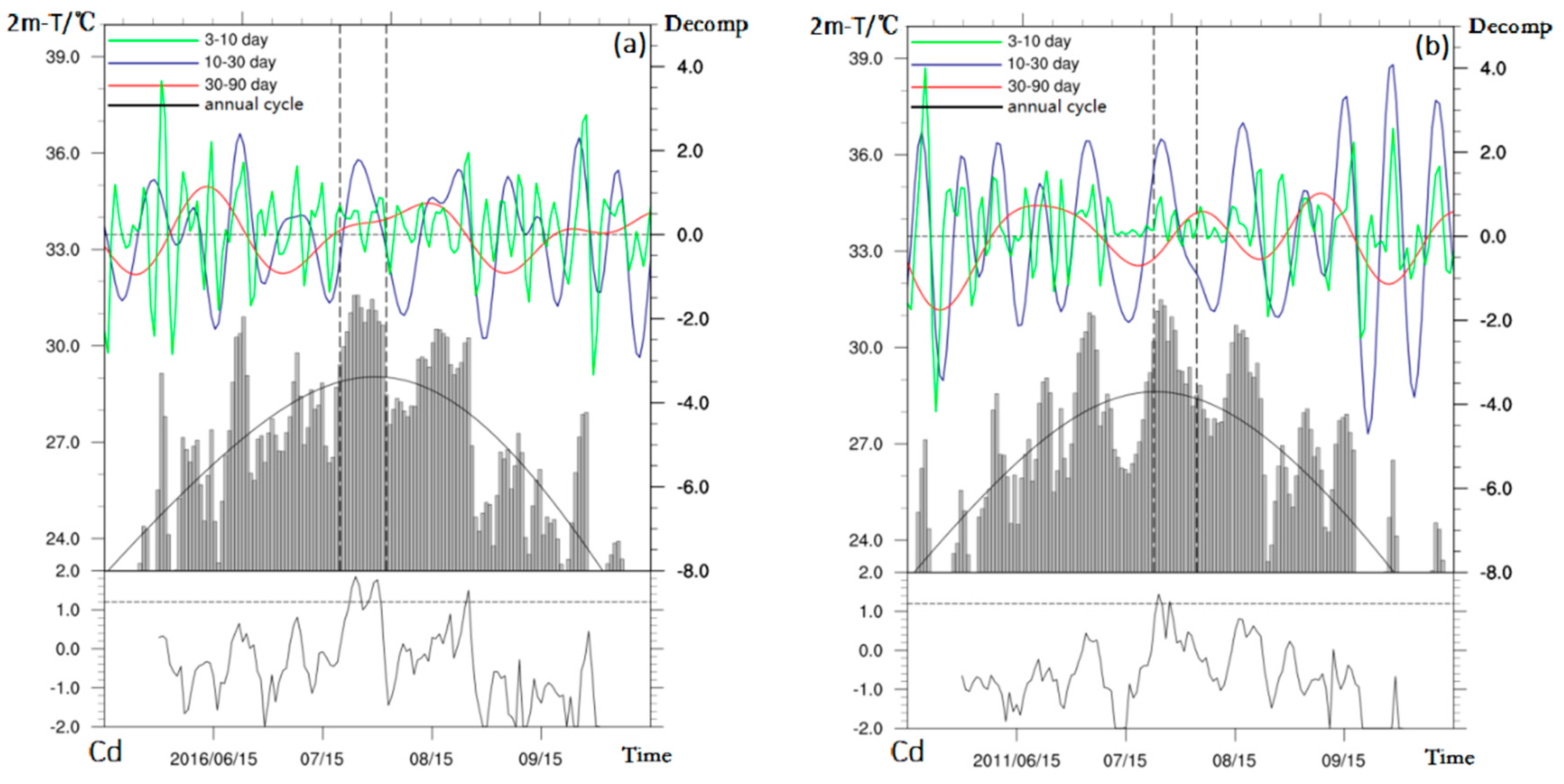
4.1. Multi-Scale Features Associated with the EHW Events

There have been many previous studies on various aspects of extreme heat-waves [25,26,27,28,29,30]. However, little is known on how variability of different time-scales acts synthetically to produce the most severe extreme heat-wave in SC as identified in the preceding section. To unravel the controlling factors of different time-scale variability on the 11 EHW events, the 2 m air temperature of the year in which the EHW occurred was decomposed into 3–10-day synoptic disturbances, 10–30-day, and 30–90-day intra-seasonal variability (ISV) by using the Butterworth band-pass filter [31]. For long-term events persisting longer than 15 days (Figure 1), the onsets of the EHW events largely correspond to the peaks or negative-to-positive transitions of both the 3–10-day and 10–30-day variability, which is consistent with the previous composite results of Chen et al. [5,6]. This result suggests that, in addition to synoptic disturbances, the 10–30-day ISV plays an important role in the onsets of long-term EHW events in SC, offering potential predictability on extended-range time-scale. At the same time, robust positive 30–90-day ISV signals exist during the course of the long-term EHW events. The ends of the long-term EHW events largely correspond to the positive-to-negative transitions of both the 30–90-day and 10–30-day ISV, which is consistent with the previous composite results of Chen et al. [5,6]. This result suggests that the persistence of long-term EHW events is dominated by 30–90-day ISV.
For short-term EHW events less than 15 days (Figure 2), the multi-scale controlling factors are different from that of long-term events. Both the 3–10-day synoptic disturbances and 10–30-day ISV contribute to the onsets and durations with the latter (former) playing a major (minor) role. This finding is also consistent with the composites of Chen et al. [5]. The time scale of 30–90 days does not seem to have much effect on short-term events, whether in the onset or in the duration.
However, the ISV signals alone could not be used to detect the occurrences of the EHW events because they exist year-around no matter what (Figure 1 and Figure 2). In order to detect the occurrence and track the temporal evolution of an EHW event in SC, a daily compound index was introduced. Unlike the integrated compound index defined in Section 2.3, the EHW daily compound index here only considers the spatial extent and intensity of individual events. Specifically, the daily compound index is defined as:
Cd = Ad + Sd,
where Cd, Ad, and Sd are, respectively, the daily compound index, and its two components: standardized daily area index and strength index. The Ad is the number of all stations with daily maximum air temperature larger than the threshold of the 90th percentile of a station (no need to be adjacent points but within the SC domain), which needs to be standardized with the standard deviation used to standardize the A(i) in Equation (2). Along the same line, Sd is the daily strength index formed by accumulating the differences between the maximum daily air temperature and 35 °C for all stations exceeding the threshold of 90th percentile (if the maximum daily air temperature is below 35 °C, then providing a negative value and the stations in this case do not need to be adjacent), then divided by the number of the stations and standardized by the value used to the S(i) in Equation (2).
The standardized values of Ad and Sd are between −1 and 1. Therefore, the value of the EHW daily compound index fluctuates between −2 and 2. The higher the daily compound index, the greater the heat-wave area and intensity in SC on that day, the more likely an EHW event will occur. By analyzing the daily compound index of the top 11 EHW events, it was found that the probability of EHW events is extremely high when the daily compound index reaches to around 1.2. Figure 1 and Figure 2 indicate that when the daily compound index is greater than 1.2, it corresponds to the onset time of the EHW events in SC. In addition, the EHW daily compound index largely remains greater than 1.2 during the event, eventually dropping rapidly to negative values at the end of the event. Whether it is a long-term event greater than 15 days or a short-term event less than 15 days, the EHW daily compound index serves as a useful indicator for the occurrence and onset time of an EHW event.
EHW events in SC mainly occur in July and August. Although the regionally-averaged 2 m air temperature in July and August is always the highest in a year, during some periods of July and August, it may reach beyond the climatological annual cycle (Figure 1 and Figure 2), these periods do not automatically qualify as EHW events. It should be assessed in combination with other important factors: e.g., the daily compound index, synoptic and intra-seasonal variability. When the daily compound index reaches about 1.2, the regionally-averaged air temperature is apparently higher than the climatological annual cycle, the 3–10-day and 10–30-day variability is peaking or transitioning from negative to positive anomaly, the occurrence probability of EHW events in SC is extremely high.
Through decomposition and analysis of the air temperature in SC, it was found that the variability of different time scales may have complementary roles on shaping the EHW events. However, what are the precursory signals of the EHW events in SC? How will multi-scale variability act synthetically to affect the characteristics of the EHW events? The following subsections will be devoted to addressing these questions. Revealing the precursory signals of the EHW events and understanding their controlling factors are essential to the prediction of the EHW events and to mitigate their societal-economic impacts.

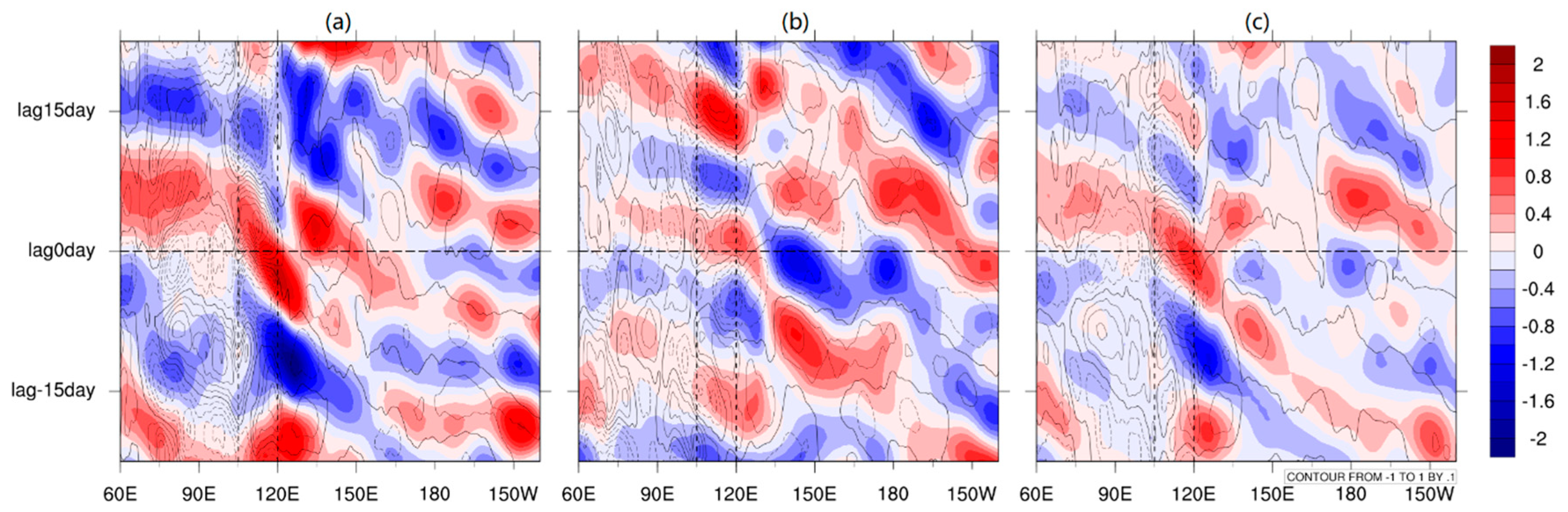
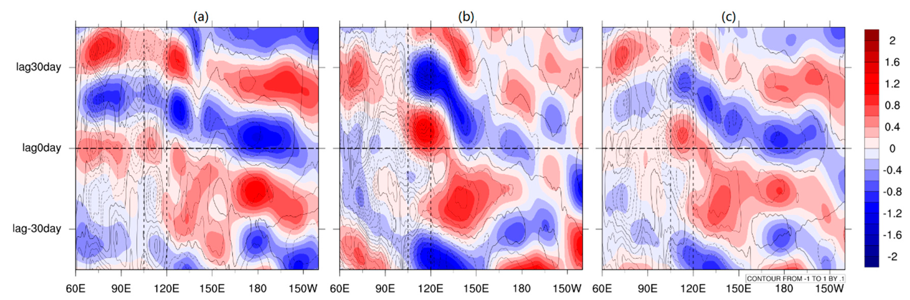
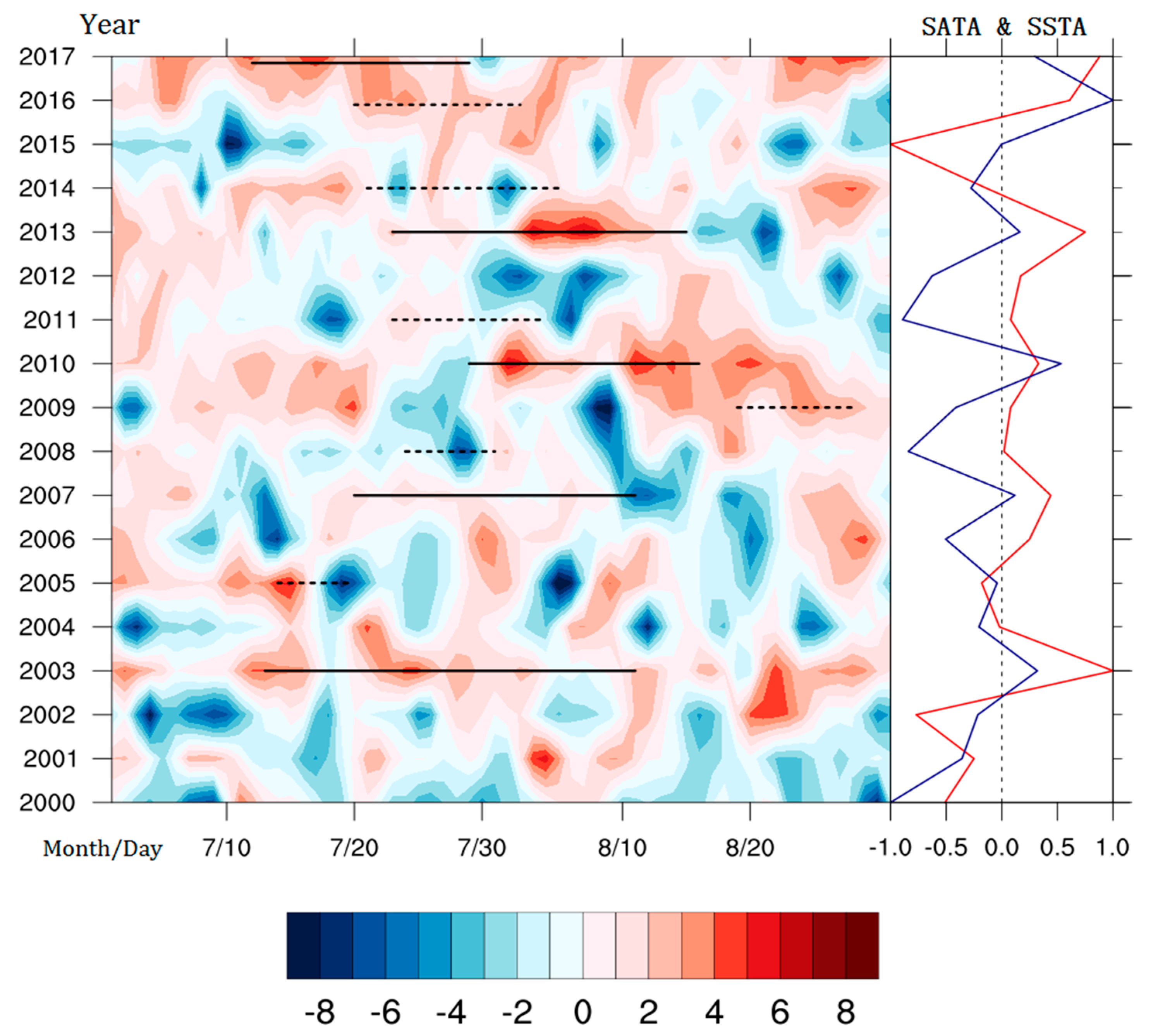
4.2. Impacts of Intra-Seasonal Variability on the Life-Cycle of the EHW Events

Previous studies with individual cases revealed that anticyclonic circulations associated with anomalous high-pressure systems are the major cause of EHW events [32,33]. Li et al. [14] found that the time series of 500 hPa geopotential height anomaly averaged over the middle and lower reaches of the Yangtze River (26.4° N~34.2° N, 105° E~122° E) had high positive correlation with the total heat-wave for all the stations in the region during 1979–2013 summers.
Since the air temperature anomaly in SC is well correlated with the 500 hPa geopotential height anomaly [2,3], it is interesting to see whether the early signals of EHW events can be found from the 500 hPa geopotential height anomaly. As indicated from the temporal analyses (Figure 1 and Figure 2), the EHW events in SC are strongly associated with ISV. We also know that the associated ISV may come from different sources [34,35,36]: The westward-propagating ISV from the western Pacific; the northward-propagating ISV from the equatorial region. In the following analyses, we make respective composites of surface air temperature and 500 hPa geopotential height anomalies associated with 10–30-day and 30–90-day ISV for the short-term only, long-term only, and all top 11 EHW events to explore how these known ISVs will impact the EHW events.
It was found that, during the onsets of short-term (Figure 3a), long-term (Figure 3b), and all EHW (Figure 3c) events, the composite positive surface air temperature anomalies in SC coincide with the positive 500 hPa geopotential height anomalies on the 10–30-day time scale. The positive anomaly of short-term events is the strongest (Figure 3a), and the duration of short-term events is basically controlled by the positive anomaly of 500 hPa geopotential height associated with the 10–30-day ISV. It is worth mentioning that for long-term events, 15 days after the onsets of the events, another positive anomaly of geopotential height reemerges in the study region, which helps maintain the long-term EHW events. For both the short-term and long-term composites (Figure 3a,b), particularly the all-case composite (Figure 3c), the positive 500 hPa geopotential height anomalies can be traced back into the western Pacific. In the composition of all events (Figure 3c), the signal of positive anomaly of 500 hPa geopotential height exists more than 15 days before the event onset. The positive anomaly at about 150° W propagates westward all the way to the study area on the EHW onset day. Apparently, westward-propagating 10–30-days ISV from the western Pacific is a potential precursory signal for the EHW events in SC with a lead time of one-to-two weeks [5,6].
The 500 hPa geopotential height anomalies of 30–90-day ISV have little effect on short-term EHW events (Figure 4a). However, for long-term EHW events, the 500 hPa geopotential height anomaly of 30–90-day affects the whole period (Figure 4b). The duration of the long-term EHW event is basically overlapped with the 500 hPa geopotential height positive anomalies of 30–90-day ISV. Averaging all the EHW events together, the positive anomaly of surface air temperature within the study area is also co-located with the positive anomaly of 500 hPa geopotential height (Figure 4c). Similar to the 10–30-day ISV, the westward-propagating 30–90-day ISV is also a potential precursory signal of the EHW events in SC with a lead time of about one month. In particular, the 30–90-day ISV has a strong effect on the persistence of long-term events [6].
In order to investigate whether the EHW events have precursory signals in the north–south directions, Figure 5 gives the hovmoller diagrams of the temporal-meridional distribution of the zonal mean surface air temperature and 500 hPa geopotential height anomalies of 10–30-day ISV in SC. For short-term EHW events, the positive anomalies of surface air temperature and 500 hPa geopotential height well match each other during the events (Figure 5a). The initial signal of positive geopotential height anomaly first appears at 20° N about 7 days before the onset. It gradually propagates northward to the study area to initiate the onsets of the EHW events. However, there is no apparent northward-propagating 10–30-day ISV signal in association with the onsets of long-term EHW events (Figure 5b). On the lag0 day of the events, there was a weak positive anomaly spreading between 10° N and 30° N. The positive anomalies of surface air temperature and 500 hPa geopotential height do mark the beginning of the EHW in the study area. It is noteworthy that, for the long-term events, there was another positive anomaly of the geopotential height in the lag15 day, which is consistent with that in Figure 3. For the composite of all events (Figure 5c), the onset process is primarily a reflection of the short-term events (Figure 5a) with robust northward-propagating precursory signal of 500 hPa geopotential height anomaly, but not another positive signal as shown in the long-term events. The above results suggest that, for short-term events, precursory signals from 10–30-day ISV exist in both the western Pacific and equatorial regions; while only over the western Pacific for long-term events.
Figure 6 examines the possible impacts of 30–90-day ISV on the EHW events in SC on the north–south direction. For the short-term events (Figure 6a), no apparent precursory signal exists; but the very weak positive anomaly of the 500 hPa geopotential height associated with the EHW events is significantly amplified on the way towards the middle and lower reaches of the Yangtze River. For the long-term events (Figure 6b), robust positive anomaly of geopotential height appears a few days before the onset, co-existing with the EHW events for more than 15 days, then propagating further north to impact the middle and lower reaches of the Yangtze River. The composite of all events (Figure 6c) also shows a moderate signal over the study region with amplified impact northward.
In the above analyses, we revealed that westward (northward)-propagating ISV from the western Pacific (equatorial region) plays a dominant (supportive) role in the occurrences of EHW events in SC. To what degree are these ISV signals connected with the eastward-propagating tropical planetary-scale Madden–Julian Oscillation [37]? Figure 7a,b shows the along-equatorial composite hovmoller diagrams of OLR and (200 hPa–850 hPa) velocity potential anomalies in association, respectively, with 10–30-day and 30–90-day ISVs averaged between 30° S and 30° N. On the 10–30-day time scale (Figure 7a), the onset period of the composite EHW events corresponds to the positive anomalies of OLR and (200 hPa–850 hPa) velocity potential. The action centers shift to the east of the SC, suggesting a strong connection with the western Pacific subtropical high. The strong subsidence in association with positive OLR and velocity potential anomalies favors clear sky and the formation of an extended heat-wave in SC. It is worth pointing out that the positive 10–30-day ISV signals affecting the SC in Figure 7a are mostly stationary, not resulting from any eastward-propagating precursor on this time scale. This may be connected with the suppressed phase of the 30–90-day MJO before the onset (Figure 7b) through the emanating westward (Figure 3)- and northward (Figure 5)-propagating intraseasonal disturbances [35,38].
There are robust eastward-propagating MJO signals in association with the EHW events in SC (Figure 7b). Two suppressed periods of MJO appear, respectively, before and after the onsets of the EHW events. Therefore, the direct contribution of MJO on EHW events in SC is not for initiation but for their maintenance in particular for the long-term events. At the same time, the 30–90-day MJO may also influence the EHW events in SC, indirectly, through emanating westward (Figure 4)- and northward (Figure 6)-propagating ISV disturbances, respectively, from the western Pacific and equatorial region [35,38].
To further reveal the possible connections among different ISV components and their impacts on the EHW events in SC, the composite spatial-temporal evolutions of OLR, (200 hPa–850 hPa) velocity potential, and divergent wind anomalies are given in Figure 8 and Figure 9, respectively, for 10–30-day and 30–90-day ISV. On 10–30-day time scale, at about 12 days before the EHW (Figure 8a), there is a positive anomalous center of OLR and velocity potential in the western equatorial Pacific near the island of New Guinea, which may be an emanated 10–30-day ISV disturbance from the eastward-propagating MJO suppressed phase (Figure 7 and Figure 9a). At the same time, a negative OLR anomalous belt presents at the northwest of the positive OLR anomalous center, extending from the eastern equatorial Indian Ocean to the east of the Philippines with negative anomalies of potential velocity over a broader region. Consistent with Figure 3c, the positive anomalies in the western equatorial Pacific propagate northwestward in the following days (Figure 8b,c). About 3-days before the EHW onset (Figure 8d), the positive OLR and velocity potential anomalous center reaches 15° N around the Philippines and are significantly amplified by strong easterly shear of the Asian summer monsoon [39]. At the onset day of the EHW (Figure 8e), SC is in the center of positive anomalies of velocity potential and OLR, as well as the strong convergence of upper-level winds. Therefore, SC is controlled by subsidence. On the third day after the onset of the EHW events (Figure 8f), the positive anomalies of the 10–30-day ISV begin to weaken gradually. On the lag6 days (Figure 8g), the SC is already covered with the negative velocity potential and OLR anomalies.
For 30–90-day ISV (Figure 9), the associated velocity potential anomalies exhibit planetary-scale eastward propagation as has been shown in many previous studies [40,41,42]. Along with the eastward-propagating planetary-scale velocity potential anomalies, the alternative convective-and-suppressed phases move northeastward to modulate the evolutions of the Asian summer monsoon [13,14]. At about 10 days before the EHW onsets, the positive OLR and velocity potential anomalies in association with previous suppressed phase (Figure 7b), although very weak, have reached the SC (Figure 9a). As the negative velocity potential anomalies move eastward, the positive OLR anomalies persist over the SC until lag10 days (Figure 9b–e), significantly contributing to the onset and persistence of the EHW events [13,14]. In next two pentads (Figure 9f,g), the second suppressed phase of the 30–90-day ISV (Figure 7b) has propagated from the tropical Indian Ocean to directly affect the Asian continent, including the SC, which also contributes to the persistence of the EHW events.

4.3. Why Some Specific Years Are Favored for the Occurrences of the EHW Events?

Figure 10 shows the evolutions of domain-mean daily geopotential height anomalies over SC from 2000 to 2017 in July and August. It can be seen that the long-term EHW events correspond well with the positive anomalies of geopotential height. As can be seen from the right panel of Figure 10, the peak values of the standardized domain-mean air temperature of July and August in SC from 2000 to 2017 are well correlated to the years with long-term EHW events. The high correlation between the occurrences of long-term EHW events and regional inter-annual variability of air temperature and geopotential height motivated us to search for possible remote impact factors. After checking the global SSTA in the preceding 12 months of all 11 EHW events, we noticed that key common features are the positive SSTA over the western North Pacific in summer and the equatorial eastern Pacific in the preceding winter. For some EHW events, there is also precursory positive SSTA over the Indian Ocean. These findings are largely consistent with Deng et al. [7]. Based on these results, we defined a yearly SSTA index for 18 years from 2000 to 2017. The index standardizes the addition of the mean SSTA of the western North Pacific (averaged over 10° N–30° N, 120° E–140° E) in May and June as well as that of the eastern Pacific (averaged over 5° S–5° N, 130° W–170° W) in the preceding winter (December, January and February). From Figure 10, it can be seen that all the long-term EHW events occur in the years with the SSTA index greater than zero. Therefore, on the interannual time scale, the SSTA index defined here can serve as a potential seasonal predictor for the occurrences of long-term EHW events in a peak summer of SC. The underlying physical processes connecting the SSTA variability to the EHW events deserve further research, which is beyond the scope of the present study.

5. Concluding Remarks and Discussion

In this study, we described a new method to identify a heat-wave in SC, and then selected 43 heat-wave events in 2000–2017. Based on the impact area, duration, and strength of heat-wave events, a compound index of heat-waves was defined to quantify the overall intensity of heat-wave events in SC. The top 11 heat-wave events with the compound index greater than one were selected to study the multi-scale controlling factors of the EHW in SC. The 2 m air temperature, 500 hPa geopotential height, OLR, velocity potential anomalies and associated decompositions (annual cycle, 3–10-day synoptic disturbances, 10-to-30-day and 30-to-90-day ISV) were analyzed to reveal the multi-scale spatial-temporal variations shaping the EHW events. This pilot study provides a multi-scale perspective for further studies of the EHW events in China. The major findings of our study are summarized in the following:
(1) A daily compound index of heat-waves that combines the spatial extent and strength of the heat-wave was established to track the outbreak of the EHW events in SC. The higher the daily compound index, the greater the heat-wave area and intensity in SC on that day. The probability of EHW events is extremely high when the daily compound index reaches around 1.2. This daily compound index serves as a useful indicator for the occurrence and onset time of an EHW event.
(2) The synoptic variability and 10–30-day ISV induce the onsets of the EHW events in SC; the 30–90-day ISV is the key to the persistence of the EHW events [5,6]. About 12 days before the onset of the EHW in SC, the 10–30-day positive anomalies of velocity potential and OLR appear near the equatorial western Pacific, which then propagate northwestward. At the same time, the 30–90-day suppressed phase propagates northeastward from the Indian Ocean to the South China sector [13,14] to influence the development of the EHW events. The occurrence of the EHW in SC is coincident with the arrivals of 10–30-day and 30–90-day intra-seasonal signals (e.g., the anomalies of 500 hPa geopotential height and OLR) propagating from the east and south. Therefore, monitoring these precursory ISV signals and the daily compound index together can offer an expert early-warning system of the EHW events in SC on the extended-range time scale.
(3) On the interannual time scale, it was found that all long-term EHW events in SC occurred in the years with robust warming of the western North Pacific in early summer and warming of the equatorial eastern Pacific in the preceding winter [7]. An interannual SSTA index, which adds the SSTA over the above two regions together, could serve as a useful seasonal predictor of the EHW occurrence in SC at least one-month ahead. The underlying physical processes need further investigations.
These findings enrich our understanding of the objective identification and multi-scale controlling factors of the EHW events in SC. Further in-depth studies and numerical experiments are needed to reveal and quantify the respective roles of multi-scale processes in shaping individual EHW events. Empirical models based on our findings can be developed to quantitatively assess the forecasting capability of the EHW events in SC and to compare with the performances of state-of-art subseasonal-to-seasonal prediction models [43,44,45].
Under the impacts of global warming, EHW events are expected to further increase in China and around the world. The understanding of the processes driving the regional features of the EHW events under a changing climate has drawn much attention around the world [46,47,48,49,50,51]. It has been recognized that changes in regional circulation patterns may affect long-term variations of EHW over some regions [52]. In order to predict future EHW changes more reliably on a regional scale, it is necessary for models to reliably capture regional circulation changes and their relationship with surface air temperature. Since the territory of China covers vast longitudinal and latitudinal ranges with diverse weather and climate regimes, the major modes that affect extremes in different regions can be very different. Some previous studies have found that the EHW in specific regions can result from various types of circulation anomalies [53,54,55]. Even the key circulations affecting nearby sites could be quite different [56]. The bottom-up approach used in this study is a viable method that can be adopted to other regions to reveal the multi-scale factors in shaping regional EHW events and to develop multi-scale synthetic expert systems for the subseasonal-to-seasonal monitoring and prediction of regional EHW events.

Author Contributions

J.-X.F. and W.C. conceived and designed the study; W.C. analyzed the data and discussed the results with J.-X.F. and G.L.; W.C. and J.-X.F. wrote the paper. All authors have read and agreed to the published version of the manuscript.

Funding

This work was jointly supported by the startup fund of Fudan University, the China National Science Foundation under grant 41875064 and National Key Research Program and Development of China under grant 2017YFC1502302.

Acknowledgments

We heartily express our appreciation to the three reviewers for their insightful comments and suggestions, which helped to improve the manuscript significantly. We also would like to express our gratitude to the staff of the ECWMF for the ERA5. Without their diligent work, it would have been impossible for us to finish our study and this paper.

Conflicts of Interest

The authors declare no conflict of interest.

Appendix A

Figure A1. The study region and distribution of the stations.
Atmosphere 11 00668 g0a1
Table A1. The heat-wave events in southern China from 2000 to 2017.
NumberStartEndDuration (Days)Station (Number)Intensity-S(i)Index-C(i)
113 July 200311 August 2003301290.897.2171
223 July 201315 August 201324701.545.6005
320 July 200711 August 200723950.894.7251
420 July 20162 August 2016141060.893.4401
512 July 201729 July 201718790.93.2598
629 July 201016 August 201019700.873.0575
723 July 20114 August 2011131010.552.2596
821 July 20145 August 201416760.431.6505
924 July 200831 July 20088690.991.2695
1019 August 200928 August 200910990.331.1023
1114 July 200520 July 20057671.011.0619
1221 July 200029 July 20009840.570.969
1314 July 200923 July 200910451.030.8954
142 August 200410 August 20049740.620.7388
1526 July 20051 August 20057830.570.5626
1612 August 201119 August 20118550.860.4651
1710 August 201625 August 201616490.30.3902
1810 August 200619 August 200610680.40.1837
1926 June 20043 July 20048660.510.0074
2023 August 200329 August 20037560.730.0012
2123 July 200429 July 20047520.73−0.1391
221 July 201015 July 201015320.37−0.2229
2311 July 200218 July 20028650.39−0.3169
241 August 20157 August 20157370.84−0.4
2520 July 200130 July 200111410.46−0.433
2615 September 200521 September 20057360.73−0.7002
2713 August 200820 August 20088240.79−0.7908
283 July 200111 July 20019230.71−0.8331
2919 July 200626 July 20068630.08−1.1341
3011 August 200515 August 20055260.76−1.35
3127 June 20153 July 20157240.62−1.3862
322 September 20099 September 20098530.09−1.4608
3314 August 201721 August 20178360.32−1.5027
3410 July 201516 July 20157370.31−1.6774
3515 September 201021 September 20107320.17−2.1902
3622 August 201129 August 20118110.35−2.3072
3715 September 200823 September 2008926−0.05−2.5595
3820 August 200125 August 20016300.12−2.5665
3922 June 201628 June 20167300.02−2.6218
4022 July 201228 July 20127100.14−3.0341
414 September 200310 September 2003711−0.07−3.5051
4223 August 200231 August 2002927−0.54−3.7054
4311 August 201218 August 2012824−0.55−4.0203

References

  1. World Meteorological Organization (WMO). Seamless Prediction of the Earth System: From Minutes to Months; WMO-No1156; WMO: Geneva, Switzerland, 2015. [Google Scholar]
  2. Ding, T.; Qian, W.H. Statistical characteristics of heat wave precursors in China and model prediction. Chin. J. Geophys. 2012, 55, 1472–1486. (In Chinese) [Google Scholar]
  3. Tang, T.; Jin, R.H.; Peng, X.Y.; Niu, R.Y. The analysis of causes about extremely high temperature in the summer of 2013 year in the southern region. J. Chengdu Univ. Inf. Technol. 2014, 29, 652–659. (In Chinese) [Google Scholar]
  4. Wang, W.W.; Zhou, W.; Wang, X.; Fong, S.K.; Leong, K.C. Summer high temperature extremes in Southeast China associated with the East Asian jet stream and circumglobal teleconnection. J. Geophys. Res. Atmos. 2013, 118, 8306–8319. [Google Scholar] [CrossRef]
  5. Chen, R.D.; Wen, Z.P.; Lu, R.Y. Evolutions of the circulation anomalies and the quasi-biweekly oscillations associated with extreme heat events in South China. J. Clim. 2016, 19, 6909–6921. [Google Scholar] [CrossRef]
  6. Chen, R.D.; Wen, Z.P.; Lu, R.Y. Large-scale circulation anomalies and intraseasonal oscillations associated with long-lived extreme heat events in South China. J. Clim. 2018, 31, 213–232. [Google Scholar] [CrossRef]
  7. Deng, K.Q.; Yang, S.; Ting, M.F.; Zhao, P.; Wang, Z.Y. Dominant modes of China summer heat waves driven by global sea surface temperature and atmospheric internal variability. J. Clim. 2019, 32, 3761–3775. [Google Scholar] [CrossRef]
  8. Li, J.; Ding, T.; Jia, X.L.; Zhao, X.C. Analysis on the extreme heat wave over China around Yangtze River region in the summer of 2013 and its main contributing factors. Adv. Meteorol. 2015, 2015, 1–15. [Google Scholar] [CrossRef] [Green Version]
  9. Wang, W.W.; Zhou, W.; Liu, X.Z.; Wang, X.; Wang, D.X. Synoptic-scale characteristics and atmospheric controls of summer heat waves in China. Clim. Dyn. 2016, 46, 2923–2941. [Google Scholar] [CrossRef]
  10. Chen, S.Y.; Wang, J.S.; Guo, J.T.; Lu, X.D. Evolution characteristics of the extreme high temperature event in Northwest China from 1961 to 2009. J. Nat. Res. 2012, 27, 832–844. (In Chinese) [Google Scholar]
  11. Loikith, P.C.; Broccoli, A.J. Characteristics of observed atmospheric circulation patterns associated with temperature extremes over North America. J. Clim. 2012, 25, 7266–7281. [Google Scholar] [CrossRef]
  12. Gao, M.N.; Yang, J.; Wang, B.; Zhou, S.Y.; Gong, D.Y.; Kim, S.J. How are heat waves over Yangtze River valley associated with atmospheric quasi-biweekly oscillation? Clim. Dyn. 2018, 51, 4421–4437. [Google Scholar] [CrossRef]
  13. Diao, Y.F.; Li, T.; Hsu, P.C. Influence of the boreal summer intraseasonal oscillation on extreme temperature events in the northern hemisphere. J. Meteorol. Res. 2018, 32, 534–547. [Google Scholar] [CrossRef]
  14. Chen, Y.; Zhai, P.M. Simultaneous modulations of precipitation and temperature extremes in Southern parts of China by the boreal summer intraseasonal oscillation. Clim. Dyn. 2017, 49, 3363–3381. [Google Scholar] [CrossRef] [Green Version]
  15. Ding, T.; Qian, W.H.; Yan, Z.W. Changes in hot days and heat waves in China during 1961–2007. Int. J. Climatol. 2010, 30, 1452–1462. [Google Scholar] [CrossRef]
  16. Chen, R.D.; Wen, Z.P.; Lu, R.Y. Interdecadal change on the relationship between the mid-summer temperature in South China and atmospheric circulation and sea surface temperature. Clim. Dyn. 2018, 51, 2113–2126. [Google Scholar] [CrossRef]
  17. Song, L.; Wu, R.G.; Jiao, Y. Relative contributions of synoptic and intraseasonal variations to strong cold events over eastern China. Clim. Dyn. 2018, 50, 4619–4634. [Google Scholar] [CrossRef]
  18. Ding, T.; Qian, W.H. Geographical patterns and temporal variations of regional dry and wet heatwave events in China during 1960–2008. Adv. Atmos. Sci. 2011, 28, 322–337. [Google Scholar] [CrossRef]
  19. Hersbach, H.; de Rosnay, P.; Bell, B.; Schepers, D.; Simmons, A.; Soci, C.; Abdalla, S.; Alonso-Balmaseda, M.; Balsamo, G.; Bechtold, P.; et al. Operational Global Reanalysis: Progress, Future Directions and Synergies with NWP; ERA Report Series No. 27; ECMWF: Reading, UK, 2018. [Google Scholar]
  20. Stefanon, M.; D’Andrea, F.; Drobinski, P. Heatwave classification over Europe and the Mediterranean region. Environ. Res. Lett. 2012, 7, 1–9. [Google Scholar] [CrossRef]
  21. Zscheischler, J.; Mahecha, M.D.; Harmeling, S.; Reichstein, M. Detection and attribution of large spatiotemporal extreme events in Earth observation data. Ecol. Inform. 2013, 15, 66–73. [Google Scholar] [CrossRef]
  22. Russo, S.; Jana, S.; Fischer, E.M. Top ten European heatwaves since 1950 and their occurrence in the coming decades. Environ. Res. Lett. 2015, 10, 1–15. [Google Scholar] [CrossRef]
  23. Lyon, B.; Barnston, A.G.; Coffel, E.; Horton, R.M. Projected increase in the spatial extent of contiguous US summer heat waves and associated attributes. Environ. Res. Lett. 2019, 14, 1–10. [Google Scholar] [CrossRef]
  24. Zhang, L.J.; Yuan, N.W. Comparison and selection of index standardization method in linear comprehensive evaluation model. Stat. Inf. Forum 2010, 25, 10–15. (In Chinese) [Google Scholar]
  25. Zhai, P.M.; Pan, X.H. Trends in temperature extremes during 1951–1999 in China. Geophys. Res. Lett. 2003, 30, 169–172. [Google Scholar] [CrossRef]
  26. Wei, K.; Chen, W. Climatology and trends of high temperature extremes across China in summer. Atmos. Ocean. Sci. Lett. 2009, 2, 153–158. [Google Scholar]
  27. Huang, D.Q.; Qian, Y.F.; Zhu, J. Trends of temperature extremes in China and their relationship with global temperature anomalies. Adv. Atmos. Sci. 2010, 27, 937–946. [Google Scholar] [CrossRef]
  28. Qian, C.; Yan, Z.W.; Wu, Z.H.; Fu, C.B.; Tu, K. Trends in temperature extremes in association with weather-intraseasonal fluctuations in eastern China. Adv. Atmos. Sci. 2011, 28, 297–309. [Google Scholar] [CrossRef]
  29. Sun, J.Q.; Wang, H.J.; Yuan, W. Decadal variability of the extreme hot event in China and its association with atmospheric circulations. Clim. Environ. Res. 2011, 2, 199–208. (In Chinese) [Google Scholar]
  30. Wei, K.; Chen, W. An abrupt increase in the summer high temperature extreme days across China in the mid-1990s. Adv. Atmos. Sci. 2011, 5, 1023–1029. [Google Scholar] [CrossRef]
  31. Masato, M. Large-scale aspects of deep convective activity over the GATE area. Mon. Weather Rev. 1979, 107, 994–1013. [Google Scholar]
  32. Lu, R.Y.; Chen, R.D. A review of recent studies on extreme heat in China. Atmos. Ocean. Sci. Lett. 2016, 9, 114–121. [Google Scholar] [CrossRef] [Green Version]
  33. Wei, J.; Sun, J.H. The analysis of summer heat wave and sultry weather in north China. Clim. Environ. Res. 2007, 12, 453–463. (In Chinese) [Google Scholar]
  34. Xie, Y.B.; Chen, S.J.; Chang, I.L.; Huang, Y.L. A preliminarily statistic and synoptic study about the basic currents over southeastern Asia and the initiation of typhoons. Acta Meteorol. Sin. 1963, 33, 206–217. (In Chinese) [Google Scholar] [CrossRef]
  35. Wang, B.; Xie, X. A model for the boreal summer intraseasonal oscillation. J. Atmos. Sci. 1997, 54, 72–86. [Google Scholar] [CrossRef] [Green Version]
  36. Fu, J.X.; Wang, B.; Tao, L. Satellite data reveal the 3-D moisture structure of tropical intraseasonal oscillation and its coupling with underlying ocean. Geophys. Res. Lett. 2006, 33, L03705. [Google Scholar] [CrossRef] [Green Version]
  37. Madden, R.A.; Julian, P.R. Description of global-scale circulation cells in tropics with a 40–50 day period. J. Atmos. Sci. 1972, 29, 1109–1123. [Google Scholar] [CrossRef]
  38. Yasunari, T. Cloudiness fluctuations associated with the Northern Hemisphere summer monsoon. J. Meteorol. Soc. Jpn. 1979, 57, 227–242. [Google Scholar] [CrossRef] [Green Version]
  39. Teng, H.Y.; Wang, B. Interannual variations of the boreal summer intraseasonal oscillation in the Asian-Pacific region. J. Clim. 2003, 16, 3572–3584. [Google Scholar] [CrossRef] [Green Version]
  40. Lorenc, A.C. The evolution of planetary-scale 200-mb divergent flow during the FGGE year. Quart. J. R. Meteorol. Soc. 1984, 72, 401–412. [Google Scholar] [CrossRef]
  41. Knutson, T.R.; Weickmann, K.M.; Kutzbach, J.E. Global-scale intraseasonal oscillations of outgoing longwave radiation and 250mb zonal wind using Northern Hemisphere summer. Mon. Weather Rev. 1986, 114, 605–623. [Google Scholar] [CrossRef] [Green Version]
  42. Fu, J.X.; Wang, W.Q.; Ren, H.L.; Jia, X.L.; Shinoda, T. Three different downstream fates of the boreal-summer MJOs on their passages over the Maritime Continent. Clim. Dyn. 2017. [Google Scholar] [CrossRef] [Green Version]
  43. Fu, J.X.; Lee, J.Y.; Hsu, P.C.; Taniguchi, H.; Wang, B.; Wang, W.Q.; Weaver, S. Multi-model MJO forecasting during DYNAMO period. Clim. Dyn. 2013, 41, 1067–1081. [Google Scholar] [CrossRef] [Green Version]
  44. Vitart, F.; Robertson, A.W. The sub-seasonal to seasonal prediction project (S2S) and the prediction of extreme events. Npj Clim. Atmos. Sci. 2018. [Google Scholar] [CrossRef] [Green Version]
  45. Ren, P.; Ren, H.L.; Fu, J.X.; Wu, J.; Du, L. Impact of boreal summer intraseasonal oscillation on rainfall extremes in southeastern China and its predictability in CFSv2. J. Geophys. Res. Atmos. 2018, 123, 4423–4442. [Google Scholar] [CrossRef]
  46. Li, H.M.; Feng, L.; Zhou, T.J. Multi-model projection of July–August climate extreme changes over China under CO2 doubling. Part II: Temperature. Adv. Atmos. Sci. 2011, 28, 448–463. [Google Scholar] [CrossRef]
  47. Xu, Y.; Wu, J.; Shi, Y.; Zhou, B.T.; Li, R.K.; Wu, J. Change in extreme climate events over China based on CMIP5. Atmos. Ocean. Sci. Lett. 2015, 8, 185–192. [Google Scholar]
  48. Fischer, E.M.; Schär, C. Consistent geographical patterns of changes in high-impact European heatwaves. Nat. Geosci. 2010, 3, 398–403. [Google Scholar] [CrossRef]
  49. Russo, S.; Dosio, A.; Graversen, R.G.; Sillmann, J.; Carrao, H.; Dunbar, M.B.; Singleton, A.; Montagna, P.; Barbosa, P.; Vogt, J.V.; et al. Magnitude of extreme heat waves in present climate and their projection in a warming world. J. Geophys. Res. Atmos. 2014, 119, 12500–12512. [Google Scholar] [CrossRef] [Green Version]
  50. Zittis, G.; Hadjinicolaou, P.; Fnais, M.; Lelieveld, J. Projected changes in heat wave characteristics in the eastern Mediterranean and the Middle East. Reg. Environ. Chang. 2016, 16, 1863–1876. [Google Scholar] [CrossRef]
  51. Lelieveld, J.; Proestos, Y.; Hadjinicolaou, P.; Tanarhte, M.; Tyrlis, E.; Zittis, G. Strongly increasing heat extremes in the Middle East and North Africa (MENA) in the 21st century. Clim. Chang. 2016, 137, 245–260. [Google Scholar] [CrossRef] [Green Version]
  52. Horton, D.E.; Johnson, N.C.; Singh, D.; Swain, D.L.; Rajaratnam, B.; Diffenbaugh, N.S. Contribution of changes in atmospheric circulation patterns to extreme temperature trends. Nature 2015, 522, 465–469. [Google Scholar] [CrossRef] [Green Version]
  53. Cassou, C.; Terray, L.; Phillips, A.S. Tropical Atlantic influence on European heat waves. J. Clim. 2005, 18, 2805–2811. [Google Scholar] [CrossRef]
  54. Harpaz, T.; Ziv, B.; Saaroni, H.; Beja, E. Extreme summer temperatures in the East Mediterranean-Dynamical analysis. Int. J. Climatol. 2014, 34, 849–862. [Google Scholar] [CrossRef]
  55. Takane, Y.; Kusaka, H.; Kondo, H. Climatological study on mesoscale extreme high temperature events in the inland of the Tokyo Metropolitan Area, Japan, during the past 22 years. Int. J. Climatol. 2014, 34, 3926–3938. [Google Scholar] [CrossRef]
  56. Garcia-Herrera, R.; Díaz, J.; Trigo, R.; Hernández, E. Extreme summer temperatures in Iberia: Health impacts and associated synoptic conditions. Ann. Geophys. 2005, 23, 239–251. [Google Scholar] [CrossRef] [Green Version]
Figure 1. Temporal evolutions of area-mean (25° N–30° N, 113° E–118° E) daily 2 m air temperature (2 m-T) (°C, gray bars) and associated decompositions (Decomp): the climatological annual cycle across 2000–2017, 3-to-10-day synoptic disturbances, 10-to-30-day and 30-to-90-day intra-seasonal variability (the four solid lines in the top panel) along with (bottom panel) the daily compound indices (Cd) for two typical EHW events persisting more than 15 days, respectively, in (a) 2003 and (b) 2007 (Table 1). The time periods of two EHW events are highlighted within two vertical dashed lines in the two top panels of (a,b).
Atmosphere 11 00668 g001
Figure 2. Same as Figure 1, but for two typical EHW events persisting less than 15 days, respectively, in (a) 2016 and (b) 2011.
Atmosphere 11 00668 g002
Figure 3. Composite time-longitude sections of 10-to-30-day surface air temperature anomalies {contours (dashed: negative, solid: positive), CI: 0.1 °C} and 500-hPa geopotential height anomalies (shading, unit: dagpm) averaged between 20° N–30° N for the EHW events persisting less than 15 days (a), longer than 15 days (b) and (c) all EHW events. The “lag0 day” represents the onset time of individual EHW events over our study area. The domain within two vertical dashed lines highlights our study area.
Atmosphere 11 00668 g003
Figure 4. Same as Figure 3, but for 30-to-90-day intra-seasonal variability with doubled time scales for the ordinate. EHW events persisting less than 15 days (a), longer than 15 days (b) and (c) all EHW events.
Atmosphere 11 00668 g004
Figure 5. Composite time-latitude sections of 10-to-30-day surface air temperature anomalies {contours (dashed: negative, solid: positive), CI: 0.1 °C} and 500-hPa geopotential height anomalies (shading, unit: dagpm) averaged between 110° E–120° E for the EHW events persisting less than 15 days (a), longer than 15 days (b) and (c) all EHW events. The “lag0 day” represents the onset time of individual EHW events over our study area. The domain within two vertical dashed lines highlights our study area.
Atmosphere 11 00668 g005
Figure 6. Same as Figure 5, but for 30-to-90-day intra-seasonal variability with doubled time scales for the ordinate. EHW events persisting less than 15 days (a), longer than 15 days (b) and (c) all EHW events.
Atmosphere 11 00668 g006
Figure 7. Composite time-longitude sections of outgoing long-wave radiation (OLR) anomalies {contours (dashed: negative, solid: positive), CI: 1 W m−2} and (200 hPa–850 hPa) velocity potential anomalies (shading, 106 m2 s−1) of all EHW events averaged between 30° S–30° N in association with (a) 10-to-30-day and (b) 30-to-90-day intra-seasonal variability. The “lag0 day” represents the start time of individual EHW events over our target area. The domain within two vertical dashed lines highlights our target area.
Atmosphere 11 00668 g007
Figure 8. Composite horizontal spatial-temporal evolutions of 10-to-30-day OLR anomalies (shading, W m−2) and (200 hPa–850 hPa) velocity potential anomalies {contours (dashed: negative, solid: positive), CI: 0.5 106 m2 s−1} along with (200 hPa–850 hPa) divergent wind anomalies (vectors, m s−1) of all EHW events on lag days of −12 (a), −9 (b), −6 (c), −3 (d), 0 (e), 3 (f), 6 (g), 9 (h).
Atmosphere 11 00668 g008
Figure 9. Same as Figure 8, but for 30-to-90-day intra-seasonal variability on lag days of −10 (a), −5 (b), 0 (c), 5 (d), 10 (e), 15 (f), 20 (g), 25 (h) of all EHW events.
Atmosphere 11 00668 g009
Figure 10. Temporal evolutions (left part) of domain-averaged (25° N–30° N, 115° E–125° E) daily 500 hPa geopotential height anomalies in two peak summer months (July and August) from 2000 to 2017 (shading, dagpm); the horizontal black solid (dashed) lines, respectively, highlight 11 EHW events persisting longer (shorter) than 15 days. The two zig-zag lines on the right side are, respectively, standardized domain-mean (25° N–30° N, 115° E–125° E) surface air temperature anomalies (SATA) averaged through July and August (in red color) and the associated index of the sea surface temperature anomaly (SSTA) (in blue color, the detail definition of this SSTA index can be found in the context).
Atmosphere 11 00668 g010
Table 1. The top 11 extreme heat-wave (EHW) events in southern China from 2000 to 2017.
NumberStartEndDuration (Days)Station (Number)Intensity-S(i)Index-C(i)
113 July 200311 August 2003301290.897.2171
223 July 201315 August 201324701.545.6005
320 July 200711 August 200723950.894.7251
420 July 20162 August 2016141060.893.4401
512 July 201729 July 201718790.93.2598
629 July 201016 August 201019700.873.0575
723 July 20114 August 2011131010.552.2596
821 July 20145 August 201416760.431.6505
924 July 200831 July 20088690.991.2695
1019 August 200928 August 200910990.331.1023
1114 July 200520 July 20057671.011.0619

