High Resolution Air Quality Forecasting over Prague within the URBI PRAGENSI Project: Model Performance during the Winter Period and the Effect of Urban Parameterization on PM

 , , , ,
Abstract
1. Introduction
2. Methods
2.1. Models and Data
2.1.1. WRF
2.1.2. CAMx
2.1.3. Emissions
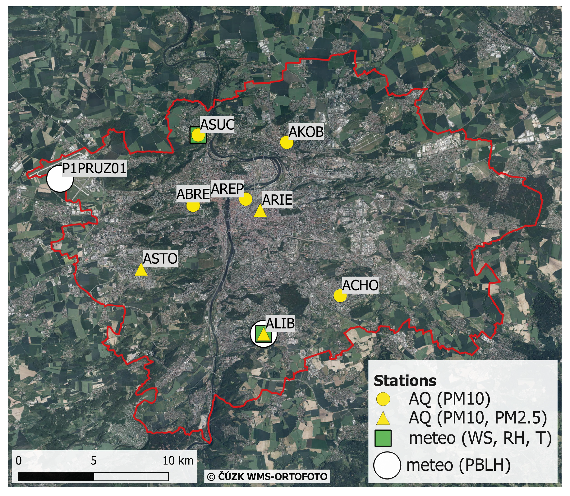
2.1.4. Air Quality Stations: Meteorology and Pollutants
2.1.5. PBL Height Retrieval from Ceilometers
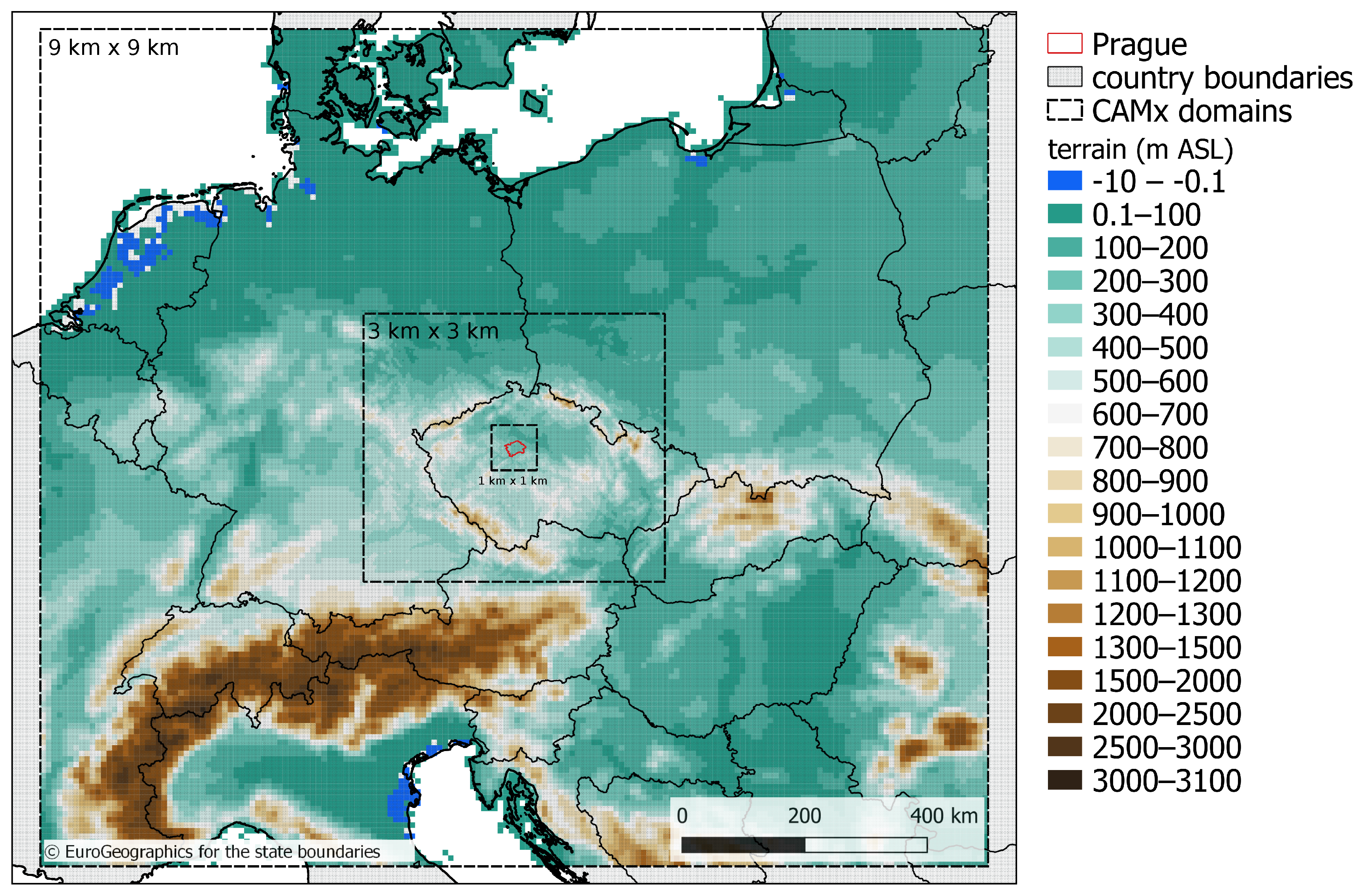
2.2. Experimental Setup
2.2.1. Model Configuration
- The “non-urbanized” configuration used the “BULK” (or SLAB) treatment of the urban land-surface. In the BULK treatment, the urban land-surface is regarded as any other flat surface with prescribed surface parameters (roughness, albedo, emissivity, etc.) representing zero-order effects of urban surfaces. It is clear that such an approach cannot fully resolve the 3D nature of the urban weather phenomenon (especially turbulence and radiation in street canyons [58]). The term “non-urbanized” here refers to the fact that these urban effects are largely ignored in the BULK approach. In this setup, there was no connection (restart) between any two successive 12 h runs described above, i.e., WRF adopted the so-called cold start concept [59].
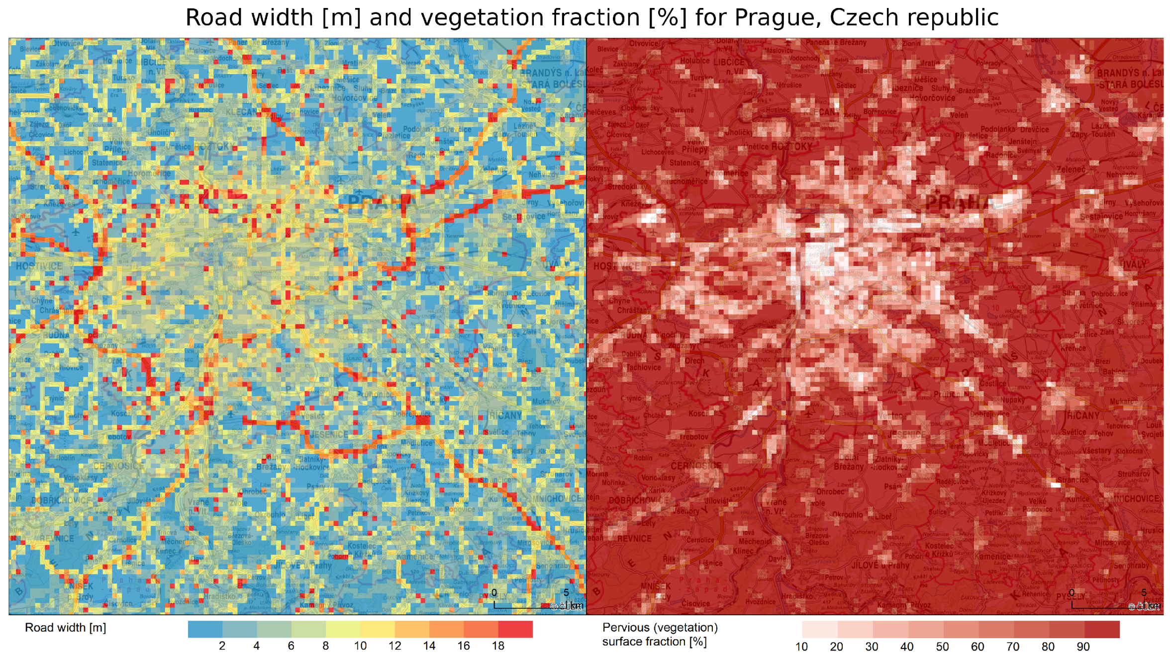
- The “urbanized” configuration of WRF had a more comprehensive treatment of the urban canopy. Instead of the BULK approach, the BEP+BEM urban canopy model was used (cf. 2.1.1). Moreover, significant changes to the land use data were made, resulting in more realistic values of variables describing the urban geometry and physical properties of surfaces (roofs, roads, walls), which influence the exchange between the urban canopy and the atmosphere. Since the state of the urban canopy submodel evolves in time, it was necessary to keep the continuity of its evolution throughout the simulation. Therefore, instead of a cold start as above, a restart was performed each 6 hours with the help of WRF’s restart capability. The restart files produced at the end of a run, needed for the restart of a successive simulation, were enriched with urban variables. Thus, the WRF run mimicked a longer term simulation, driven by analyses and keeping the continuous evolution of the variables that describe the physical state of the urban environment.
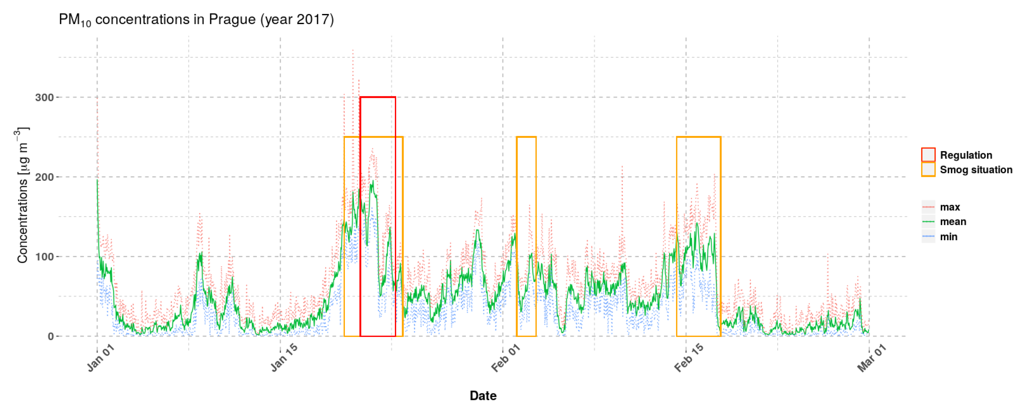
2.2.2. Simulated Period
3. Results
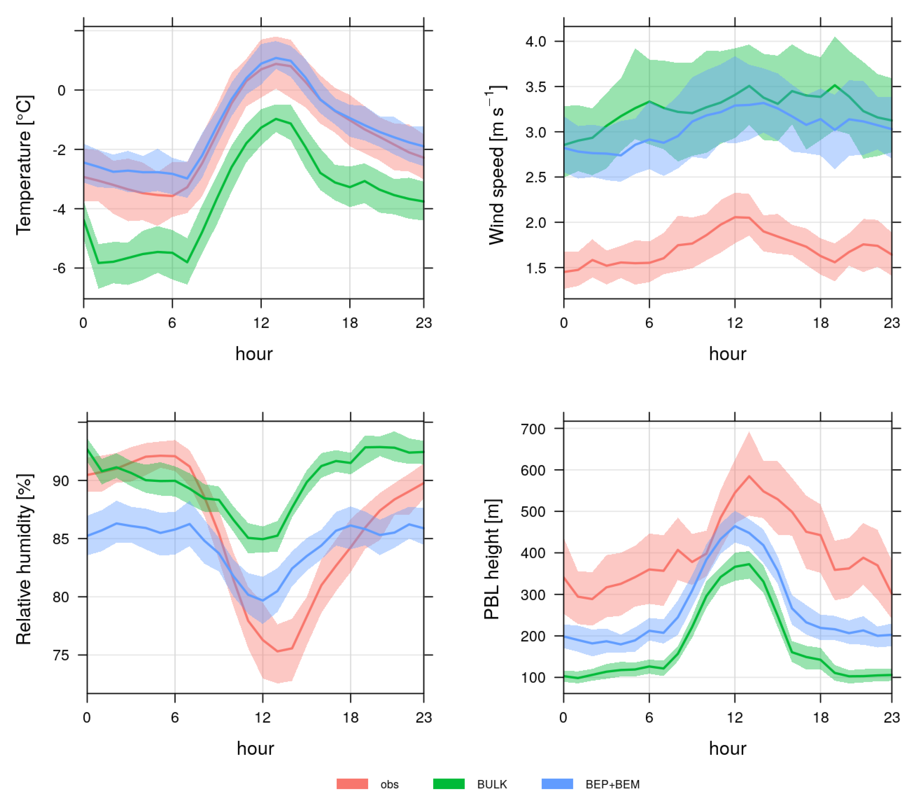
3.1. Meteorology
3.2. Air Quality
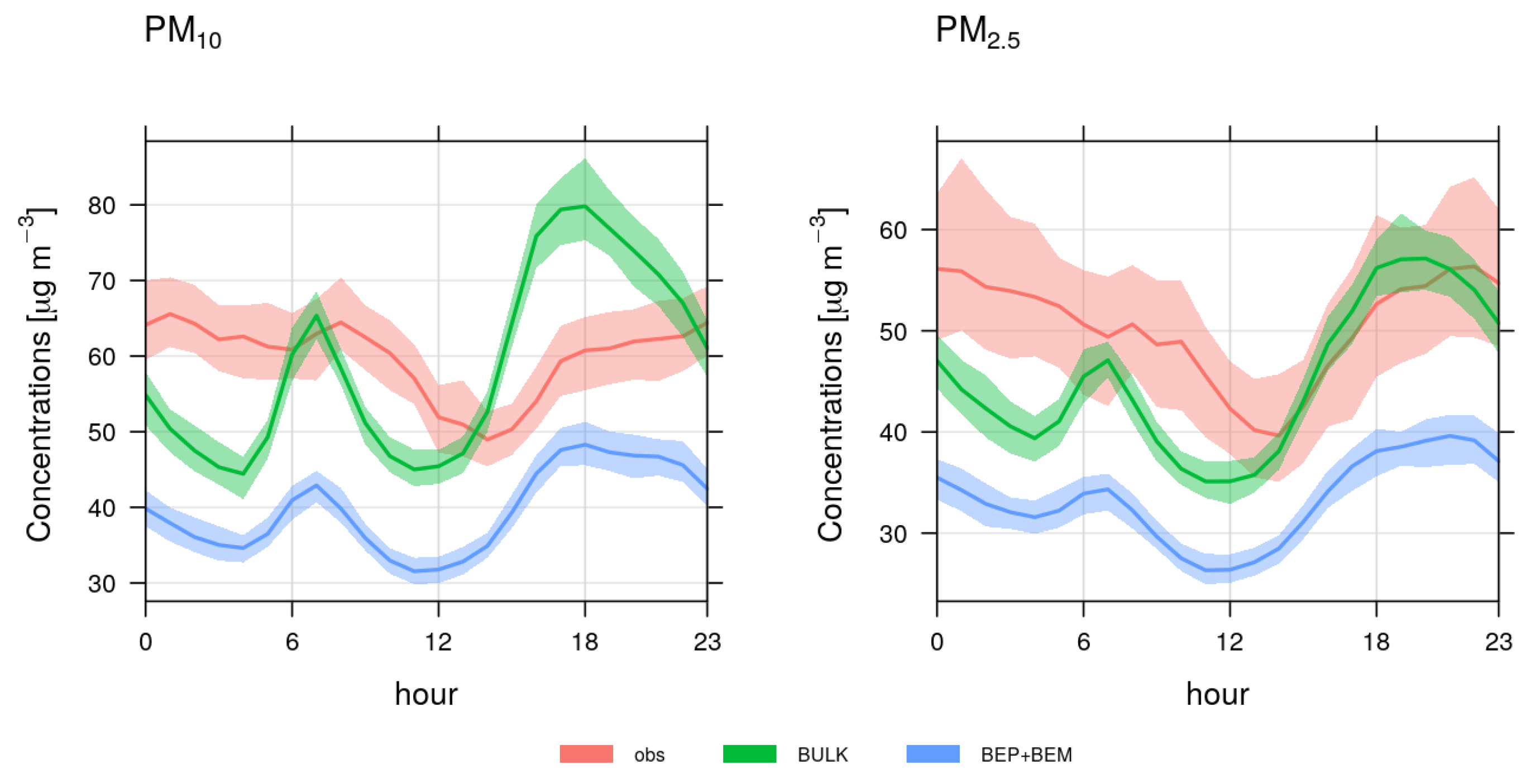
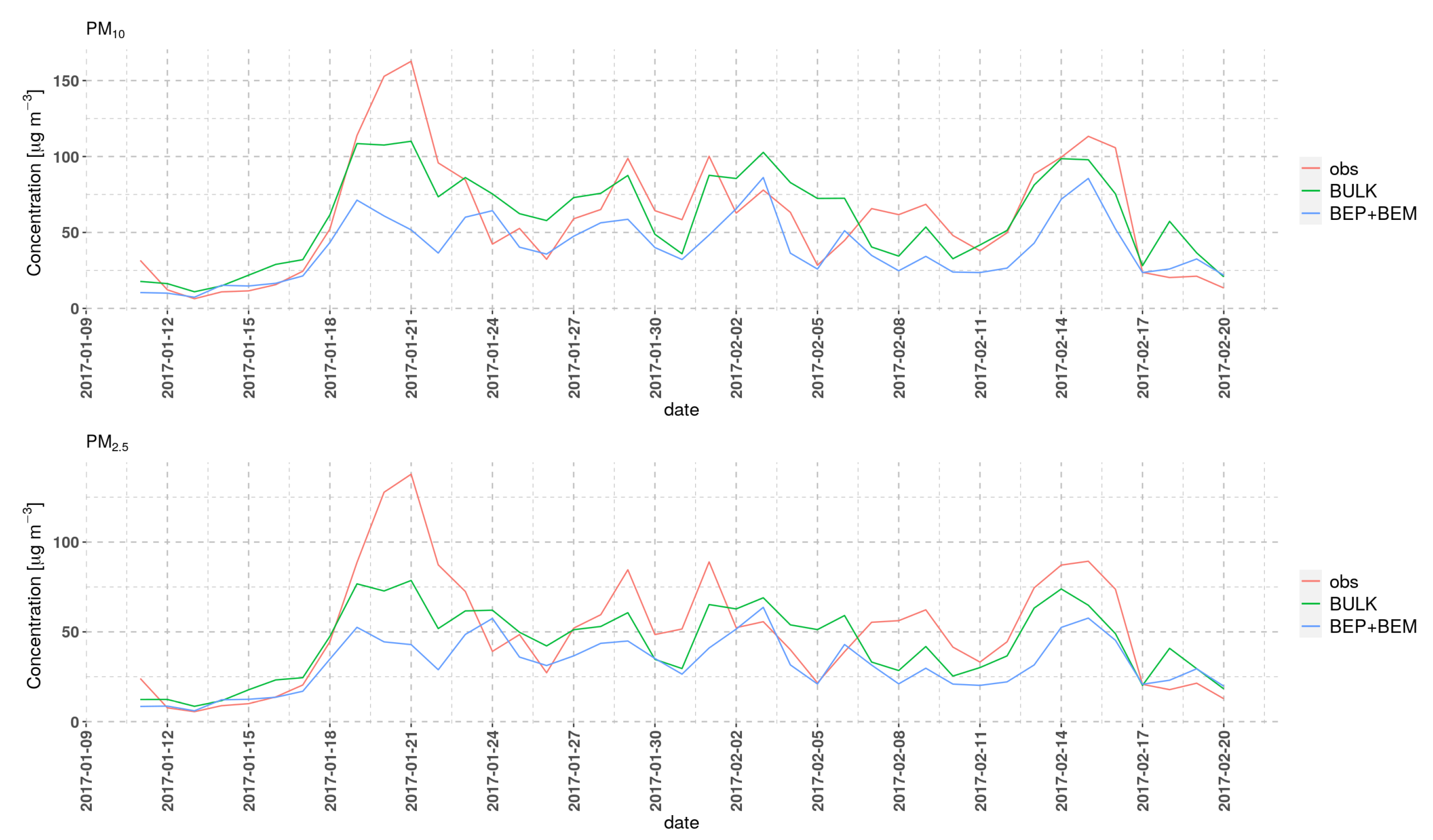
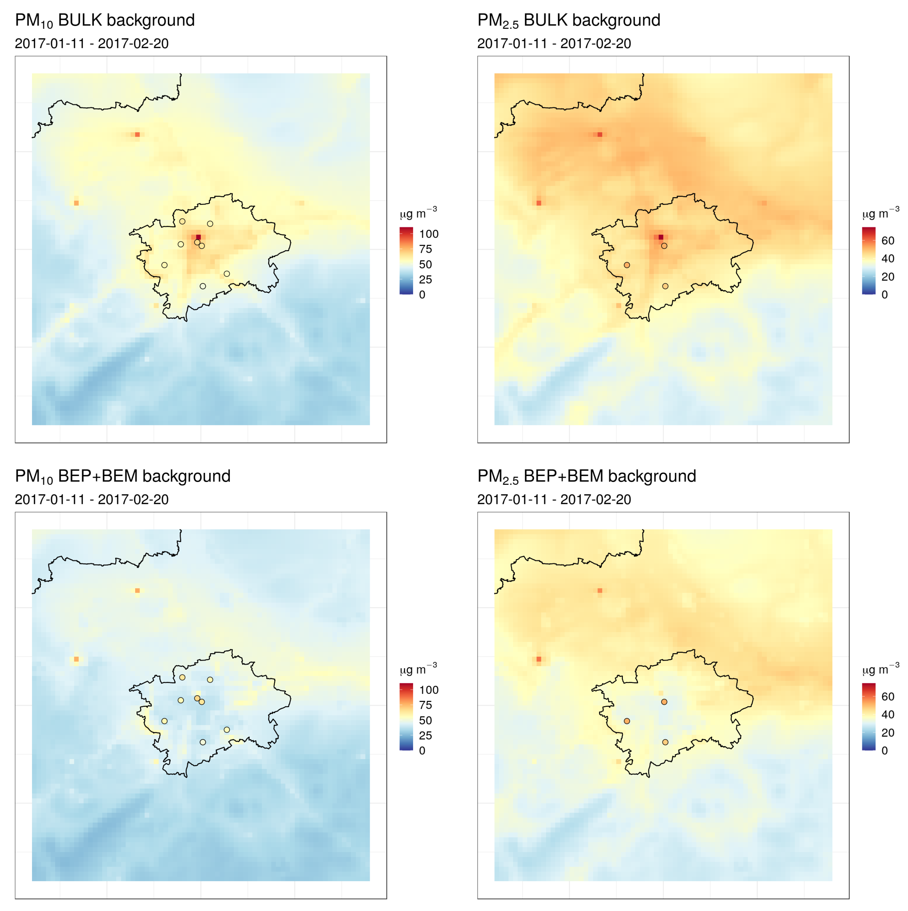
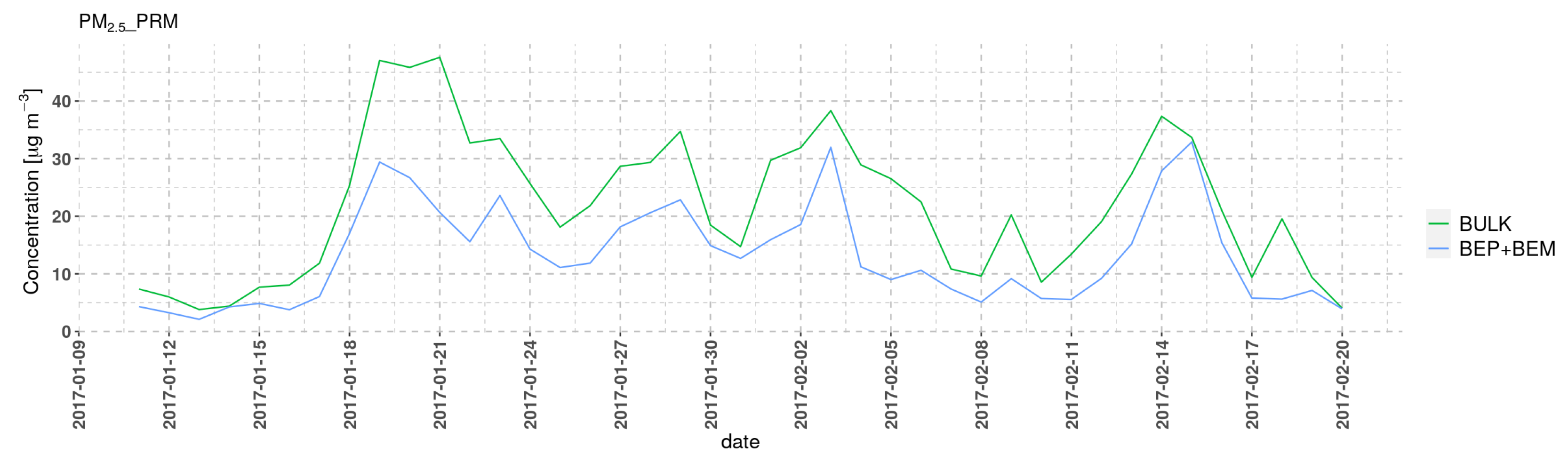
3.2.1. PM and PM
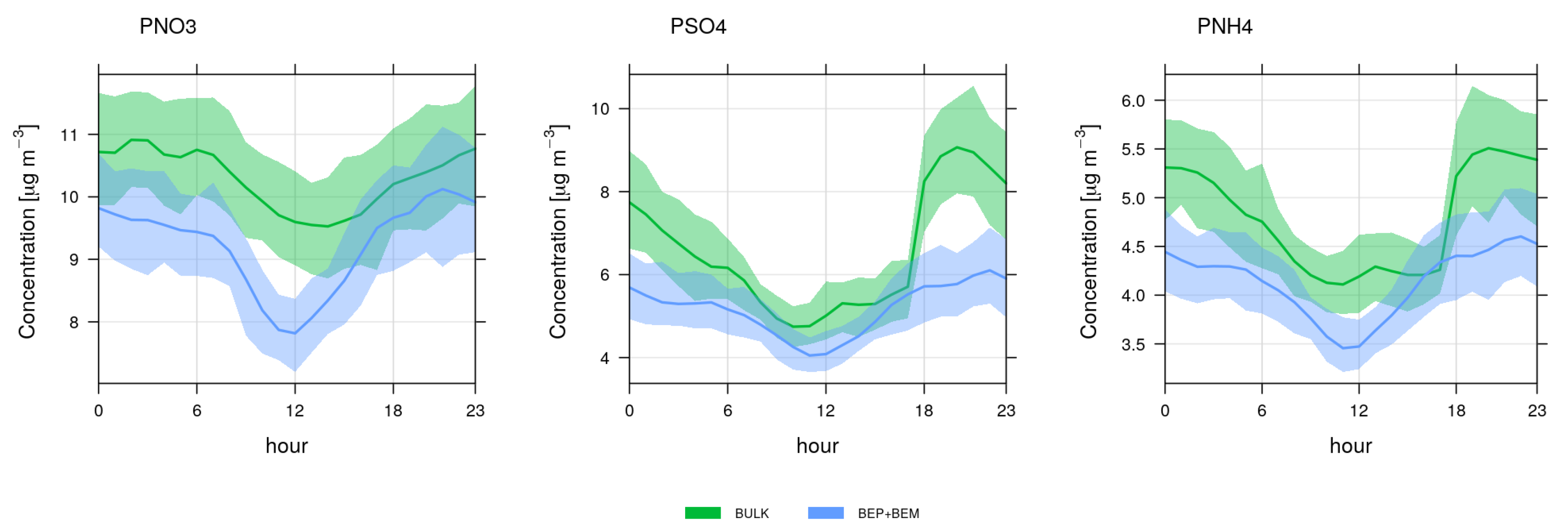
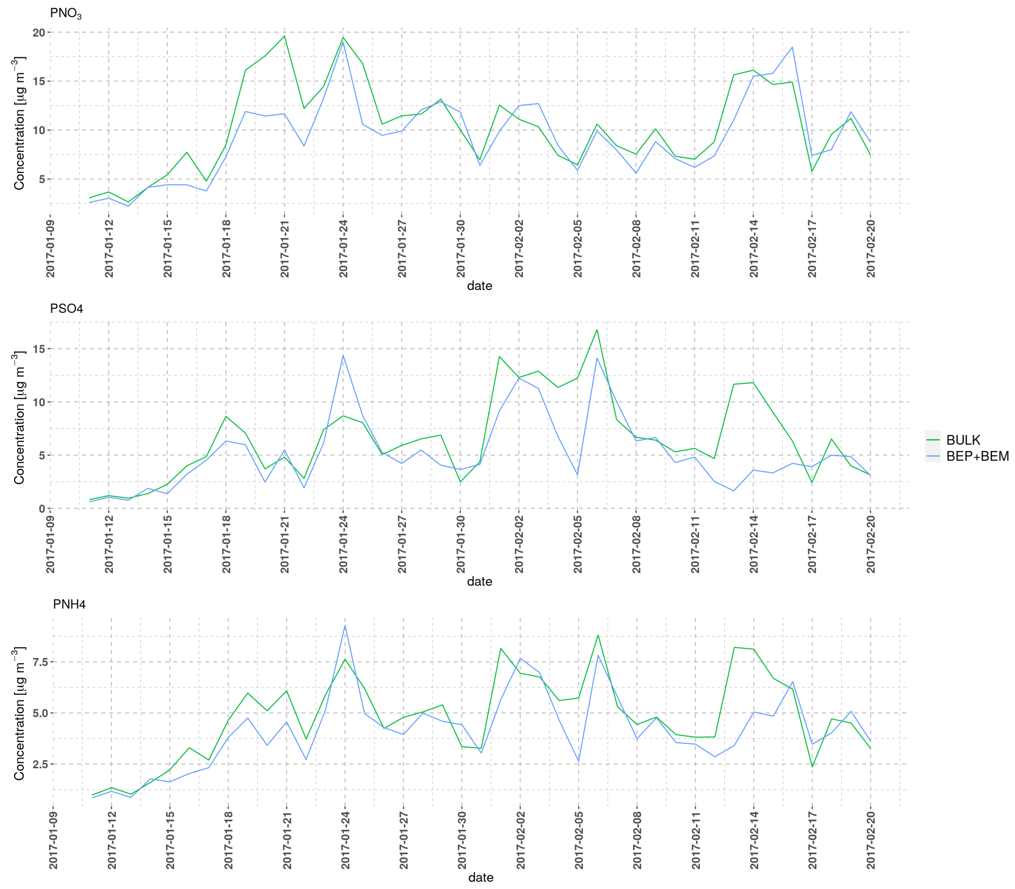
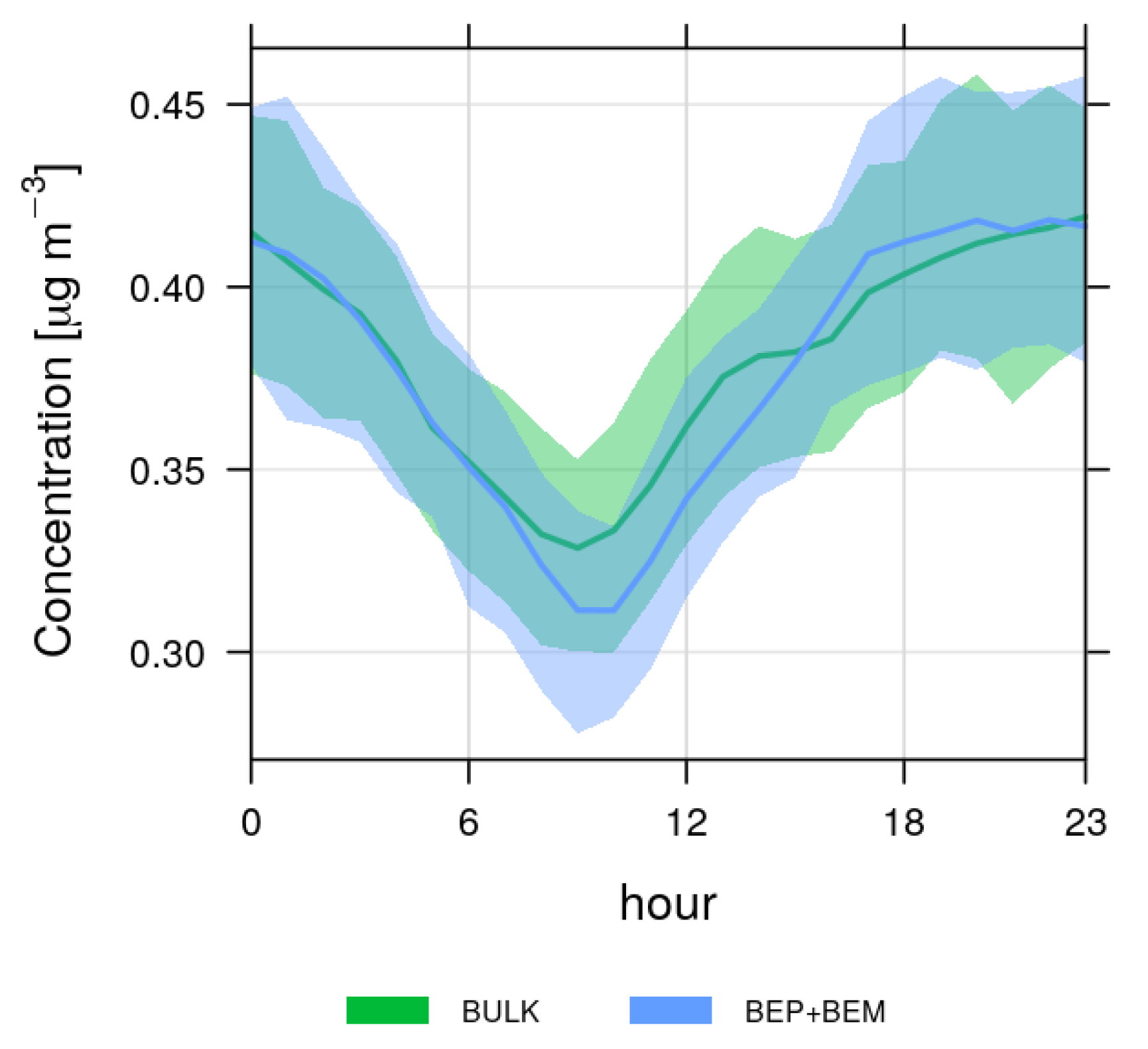
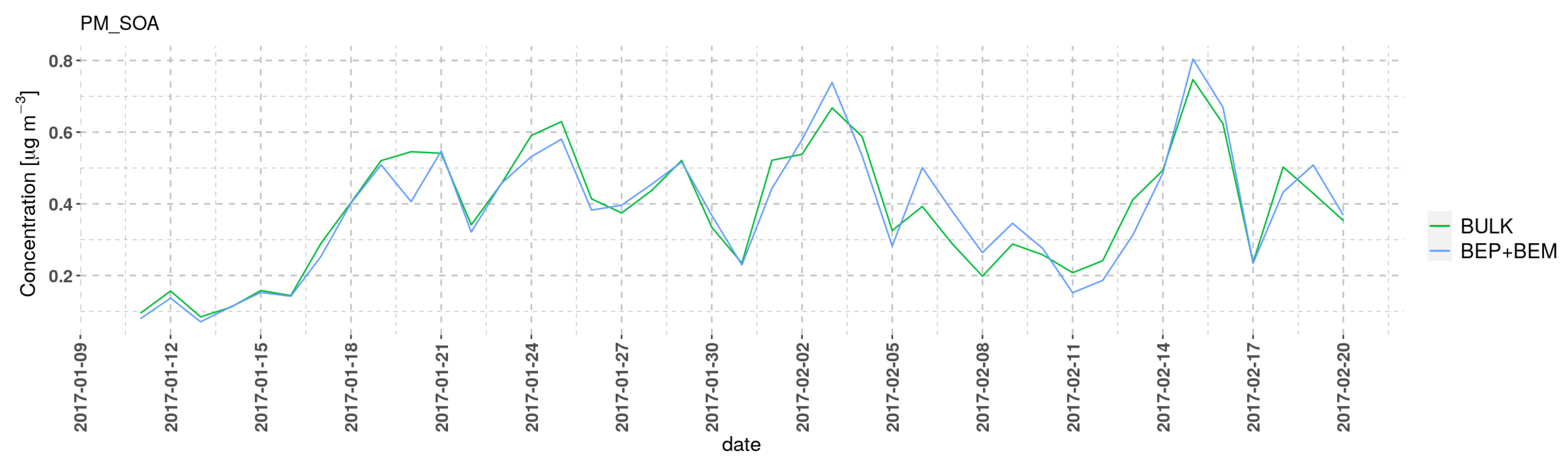
3.2.2. Analysis of the Aerosol Components
4. Discussion
5. Conclusions
Author Contributions
Funding
Acknowledgments
Conflicts of Interest
Appendix A. The Definition of the Statistical Scores
References
- Marlier, M.E.; Jina, A.S.; Kinney, P.L.; DeFries, R.S. Extreme Air Pollution in Global Megacities. Curr. Clim. Chang. Rep. 2016, 2, 15–27. [Google Scholar] [CrossRef]
- Folberth, G.A.; Butler, T.M.; Collins, W.J.; Rumbold, S.T. Megacities and climate change—A brief overview. Environ. Pollut. 2015, 203, 235–242. [Google Scholar] [CrossRef] [PubMed]
- Lawrence, M.G.; Butler, T.M.; Steinkamp, J.; Gurjar, B.R.; Lelieveld, J. Regional pollution potentials of megacities and other major population centers. Atmos. Chem. Phys. 2007, 7, 3969–3987. [Google Scholar] [CrossRef]
- Huszár, P.; Belda, M.; Halenka, T. On the long-term impact of emissions from central European cities on regional air quality. Atmos. Chem. Phys. 2016, 16, 1331–1352. [Google Scholar] [CrossRef]
- Huszár, P.; Belda, M.; Karlický, J.; Pišoft, P.; Halenka, T. The regional impact of urban emissions on climate over central Europe: Present and future emission perspectives. Atmos. Chem. Phys. 2016, 16, 12993–13013. [Google Scholar] [CrossRef]
- Huszár, P.; Halenka, T.; Belda, M.; Zak, M.; Sindelarova, K.; Miksovsky, J. Regional climate model assessment of the urban land-surface forcing over central Europe. Atmos. Chem. Phys. 2014, 14, 12393–12413. [Google Scholar] [CrossRef]
- Karlický, J.; Huszár, P.; Halenka, T.; Belda, M.; Žák, M.; Pišoft, P.; Mikšovský, J. Multi-model comparison of urban heat island modeling approaches. Atmos. Chem. Phys. 2018, 18, 10655–10674. [Google Scholar] [CrossRef]
- Kanakidou, M.; Mihalopoulos, N.; Kindap, T.; Im, U.; Vrekoussis, M.; Gerasopoulos, E.; Dermitzaki, E.; Unal, A.; Kocak, M.; Markakis, K.; et al. Megacities as hot spots of air pollution in the East Mediterranean. Atmos. Environ. 2011, 45, 1223–1235. [Google Scholar] [CrossRef]
- Im, U.; Kanakidou, M. Impacts of East Mediterranean megacity emissions on air quality. Atmos. Chem. Phys. 2012, 12, 6335–6355. [Google Scholar] [CrossRef]
- Han, W.; Li, Z.; Wu, F.; Zhang, Y.; Guo, J.; Su, T.; Cribb, M.; Chen, T.; Wei, J.; Lee, S.-S. Opposite Effects of Aerosols on Daytime Urban Heat Island Intensity between Summer and Winter. Atmos. Chem. Phys. Discuss. 2020. [Google Scholar] [CrossRef]
- Baklanov, A.; Korsholm, U.; Mahura, A.; Petersen, C.; Gross, A. ENVIRO-HIRLAM: On-line coupled modeling of urban meteorology and air pollution. Adv. Sci. Res. 2008, 2, 41–46. [Google Scholar] [CrossRef]
- Chen, F.; Kusaka, H.; Bornstein, R.; Ching, J.; Grimmond, C.S.B.; Grossman-Clarke, S.; Loridan, T.; Manning, K.W.; Martilli, A.; Miao, S.; et al. The integratedWRF/urban modeling system: Development, evaluation, and applications to urban environmental problems. Int. J. Climatol. 2011, 31, 273–288. [Google Scholar] [CrossRef]
- Sarrat, C.; Lemonsu, A.; Masson, V.; Guedalia, D. Impact of urban heat island on regional atmospheric pollution. Atmos. Environ. 2006, 40, 1743–1758. [Google Scholar] [CrossRef]
- Struzewska, J.; Kaminski, J.W. Impact of urban parameterization on high resolution air quality forecast with the GEM—AQ model. Atmos. Chem. Phys. 2012, 12, 10387–10404. [Google Scholar] [CrossRef]
- Fallmann, J.; Forkel, R.; Emeis, S. Secondary effects of urban heat island mitigation measures on air quality. Atmos. Environ. 2016, 25, 199–211. [Google Scholar] [CrossRef]
- Huszár, P.; Karlický, J.; Belda, M.; Halenka, T.; Pišoft, P. The impact of urban canopy meteorological forcing on summer photochemistry. Atmos. Environ. 2018, 176, 209–228. [Google Scholar] [CrossRef]
- Huszár, P.; Belda, M.; Karlický, J.; Bardachova, T.; Halenka, T.; Pišoft, P. Impact of urban canopy meteorological forcing on aerosol concentrations. Atmos. Chem. Phys. 2018, 18, 14059–14078. [Google Scholar] [CrossRef]
- Brasseur, G.; Jacob, D. Modeling of Atmospheric Chemistry; Cambridge University Press: Cambridge, UK, 2017. [Google Scholar] [CrossRef]
- Hidalgo, J.; Masson, V.; Gimeno, L. Scaling the Daytime Urban Heat Island and Urban-Breeze Circulation. J. Appl. Meteorol. Clim. 2010, 49, 889–901. [Google Scholar] [CrossRef]
- Ryu, Y.-H.; Baik, J.-J.; Kwak, K.-H.; Kim, S.; Moon, N. Impacts of urban land-surface forcing on ozone air quality in the Seoul metropolitan area. Atmos. Chem. Phys. 2013, 13, 2177–2194. [Google Scholar] [CrossRef]
- Ryu, Y.-H.; Baik, J.-J.; Lee, S.-H. Effects of anthropogenic heat on ozone air quality in a megacity. Atmos. Environ. 2013, 80, 20–30. [Google Scholar] [CrossRef]
- Jacobson, M.Z.; Nghiem, S.V.; Sorichetta, A.; Whitney, N. Ring of impact from the mega-urbanization of Beijing between 2000 and 2009. J. Geophys. Res. 2015, 120, 5740–5756. [Google Scholar] [CrossRef]
- De la Paz, D.; Borge, R.; Martilli, A. Assessment of a high resolution annual WRF-BEP/CMAQ simulation for the urban area of Madrid (Spain). Atmos. Environ. 2016, 144, 282–296. [Google Scholar] [CrossRef]
- Liao, J.; Wang, T.; Wang, X.; Xie, M.; Jiang, Z.; Huang, X.; Zhu, J. Impacts of different urban canopy schemes in WRF/Chem on regional climate and air quality in Yangtze River Delta, China. Atmos. Res. 2014, 145–146, 226–243. [Google Scholar] [CrossRef]
- Chen, B.; Yang, S.; Xu, X.D.; Zhang, W. The impacts of urbanization on air quality over the Pearl River Delta in winter: Roles of urban land use and emission distribution. Theor. Appl. Climatol. 2014, 117, 29–39. [Google Scholar] [CrossRef]
- Kim, Y.; Sartelet, K.; Raut, J.-C.; Chazette, P. Influence of an urban canopy model and PBL schemes on vertical mixing for air quality modeling over Greater Paris. Atmos. Environ. 2015, 107, 289–306. [Google Scholar] [CrossRef][Green Version]
- Ren, Y.; Zhang, H.; Wei, W.; Wu, B.; Cai, X.; Song, Y. Effects of turbulence structure and urbanization on the heavy haze pollution process. Atmos. Chem. Phys. 2019, 19, 1041–1057. [Google Scholar] [CrossRef]
- Tang, W.; Cohan, D.S.; Morris, G.A.; Byun, D.W.; Luke, W.T. Influence of vertical mixing uncertainties on ozone simulation in CMAQ. Atmos. Environ. 2011, 45, 2898–2909. [Google Scholar] [CrossRef]
- Huszár, P.; Karlický, J.; Ďoubalová, J.; Šindelářová, K.; Nováková, T.; Belda, M.; Halenka, T.; Žák, M.; Pišoft, P. Urban canopy meteorological forcing and its impact on ozone and PM2.5: Role of vertical turbulent transport. Atmos. Chem. Phys. 2020, 20, 1977–2016. [Google Scholar] [CrossRef]
- Wang, J.; Mao, J.; Zhang, Y.; Cheng, T.; Yu, Q.; Tan, J.; Ma, W. Simulating the Effects of Urban Parameterizations on the Passage of a Cold Front During a Pollution Episode in Megacity Shanghai. Atmosphere 2019, 10, 79. [Google Scholar] [CrossRef]
- CHMI: Air Pollution in the Czech Republic in 2018; CHMI: Prague, Czech Republic, 2019; ISBN 978--80-87577-95-0.
- CHMI: Air Pollution in the Czech Republic in 2017; CHMI: Prague, Czech Republic, 2018; ISBN 978-80-87577-83-7.
- Skamarock, W.C.; Klemp, J.B. A time-split nonhydrostatic atmospheric model for weather research and forecasting applications. J. Comput. Phys. 2008, 227, 3465–3485. [Google Scholar] [CrossRef]
- Iacono, M.J.; Delamere, J.S.; Mlawer, E.J.; Shephard, M.W.; Clough, S.A.; Collins, W.D. Radiative forcing by longlived greenhouse gases: Calculations with the AER radiative transfer models. J. Geophys. Res. 2008, 113, 2–9. [Google Scholar] [CrossRef]
- Chen, F.; Dudhia, J. Coupling an Advanced Land Surface-Hydrology Model with the Penn State-NCAR MM5 Modeling System. Part I: Model Implementation and Sensitivity. Mon. Weather Rev. 2001, 129, 569–585. [Google Scholar] [CrossRef]
- Thompson, G.; Field, P.R.; Rasmussen, R.M.; Hall, W.D. Explicit Forecasts of Winter Precipitation Using an Improved Bulk Microphysics Scheme. Part II: Implementation of a New Snow Parameterization. Mon. Weather Rev. 2008, 136, 5095–5115. [Google Scholar] [CrossRef]
- Bougeault, P.; Lacarrere, P. Parameterization of orography-induced turbulence in a mesobeta-scale model. Mon. Weather Rev. 1989, 117, 1872–1890. [Google Scholar] [CrossRef]
- Martilli, A.; Clappier, A.; Rotach, M.W. An urban surface exchange parameterisation for mesoscale models. Bound. Layer Meteorol. 2002, 104, 261–304. [Google Scholar] [CrossRef]
- Salamanca, F.; Krpo, A.; Martilli, A.; Clappier, A. A new building energy model coupled with an urban canopy parameterization for urban climate simulations—Part I. formulation, verification, and sensitivity analysis of the model. Theor. Appl. Climatol. 2009, 99, 331. [Google Scholar] [CrossRef]
- ENVIRON, CAMx User’s Guide, Comprehensive Air Quality Model with Extensions, Version 6.50; Ramboll: Los Angeles, CA, USA, 2018.
- Yarwood, G.; Rao, S.; Yocke, M.; Whitten, G.Z. Updates to the Carbon Bond Chemical Mechanism: CB05, Final Report Prepared for US EPA. 2015. Available online: http://www.camx.com/publ/pdfs/CB05_Final_Report_120805.pdf (accessed on 19 May 2020).
- Zhang, L.; Brook, J.R.; Vet, R. A revised parameterization for gaseous dry deposition in air-quality models. Atmos. Chem. Phys. 2003, 3, 2067–2082. [Google Scholar] [CrossRef]
- Seinfeld, J.H.; Pandis, S.N. Atmospheric Chemistry and Physics: From Air Pollution to Climate Change; Wiley: New York, NY, USA, 1998. [Google Scholar]
- Nenes, A.; Pandis, S.N.; Pilinis, C. ISORROPIA: A new thermodynamic equilibrium model for multiphase multicomponent inorganic aerosols. Aquat. Geochem. 1998, 4, 123–152. [Google Scholar] [CrossRef]
- Strader, R.; Lurmann, F.; Pandis, S.N. Evaluation of secondary organic aerosol formation in winter. Atmos. Environ. 1999, 33, 4849–4863. [Google Scholar] [CrossRef]
- Byun, D.W.; Ching, J.K.S. Science Algorithms of the EPA Model-3 Community Multiscale Air Quality (CMAQ) Modeling System; Office of Research and Development, U.S. EPA: Washington, DC, USA, 1999.
- Louis, J.F. A Parametric Model of Vertical Eddy Fluxes in the Atmosphere. Bound. Lay. Meteor. 1979, 17, 187–202. [Google Scholar] [CrossRef]
- Granier, C.S.; Darras, H.; Denier van der Gon, J.; Doubalova, N.; Elguindi, B.; Galle, M.; Gauss, M.; Guevara, J.-P.; Jalkanen, J.; Kuenen, C.; et al. The Copernicus Atmosphere Monitoring Service Global and Regional Emissions, Report April 2019 version [Research Report]; ECMWF: Reading, UK, 2019. [Google Scholar] [CrossRef]
- Benešová, N.; Belda, M.; Eben, K.; Geletič, J.; Huszár, P.; Juruš, P.; Krč, P.; Resler, J.; Vlček, O. New open source emission processor for air quality models. In Proceedings of the Abstracts 11th International Conference on Air Quality Science and Application, Barcelona, Spain, 12–16 March 2018; Sokhi, R., Tiwari, P.R., Gállego, M.J., Craviotto Arnau, J.M., Castells Guiu, C., Singh, V., Eds.; University of Hertfordshire: Hatfield, UK, 2018. [Google Scholar] [CrossRef]
- Passant, N. Speciation of UK Emissions of Non-Methane Volatile Organic Compounds; DEFRA: Oxon, UK, 2002.
- Builtjes, P.J.H.; van Loon, M.; Schaap, M.; Teeuwise, S.; Visschedijk, A.J.H.; Bloos, J.P. Project on the Modelling and Verification of Ozone Reduction Strategies: Contribution of TNO-MEP; TNO-report, MEP-R2003/166; TNO: Apeldoorn, The Netherlands, 2003. [Google Scholar]
- Van der Gon, H.D.; Hendriks, C.; Kuenen, J.; Segers, A.; Visschedijk, A. Description of Current Temporal Emission Patterns and Sensitivity of Predicted AQ for Temporal Emission Patterns. EU FP7 MACC Deliverable Report D_D-EMIS_1.3. 2011. Available online: http://www.gmes-atmosphere.eu/documents/deliverables/d-emis/MACC_TNO_del_1_3_v2.pdf (accessed on 19 May 2020).
- Guenther, A.B.; Jiang, X.; Heald, C.L.; Sakulyanontvittaya, T.; Duhl, T.; Emmons, L.K.; Wang, X. The Model of Emissions of Gases and Aerosols from Nature version 2.1 (MEGAN2.1): An extended and updated framework for modeling biogenic emissions. Geosci. Model Dev. 2012, 5, 1471–1492. [Google Scholar] [CrossRef]
- Vaisala’s Ceilometer CL31. Available online: https://www.vaisala.com/en/products/instruments-sensors-and-other-measurement-devices/weather-stations-and-sensors/cl31 (accessed on 19 May 2020).
- Vaisala’s Ceilometer CL51. Available online: https://www.vaisala.com/en/products/instruments-sensors-and-other-measurement-devices/weather-stations-and-sensors/cl51 (accessed on 19 May 2020).
- User’s Guide: Vaisala Boundary Layer View Software BL-VIEW; Vaisala Oyj: Helsinki, Finland, 2010.
- National Centers for Environmental Prediction/National Weather Service/NOAA/U.S. Department of Commerce. NCEP GFS 0.25 Degree Global Forecast Grids Historical Archive; National Center for Atmospheric Research, Computational and Information Systems Laboratory: Boulder, CO, USA, 2015. [CrossRef]
- Sharma, A.; Fern, H.J.; Hamlet, A.F.; Hellmann, J.J.; Barlage, M.; Chen, F. Urban meteorological modeling using WRF: A sensitivity study. Int. J. Climatol. 2017, 37, 1885–1900. [Google Scholar] [CrossRef]
- Warner, T.T. Numerical Weather and Climate, Prediction; Cambridge University Press: Cambridge, UK, 2011. [Google Scholar]
- Gillespie, A. Land Surface Emissivity. In Encyclopedia of Remote Sensing; Encyclopedia of Earth Sciences Series; Njoku, E.G., Ed.; Springer: New York, NY, USA, 2014. [Google Scholar]
- Madronich, S.; Flocke, S.; Zeng, J.; Petropavlovskikh, I.; Lee-Taylor, J. Tropospheric Ultraviolet-Visible Model (TUV), version 4.1.; National Center for Atmospheric Research: Boulder, CO, USA, 2002. [Google Scholar]
- Šopko, F.; Vlček, O.; Juras, R.; Škáchová, H. Meteorological analysis of the extensive smog situations in January and February 2017 in the Czech Republic. Meteorol. Bull. 2017, 70, 107–133. [Google Scholar]
- Oke, T.; Mills, G.; Christen, A.; Voogt, J. Urban Climates; Cambridge University Press: Cambridge, UK, 2017. [Google Scholar] [CrossRef]
- Richards, K. Observation and simulation of dew in rural and urban environments. Prog. Phys. Geogr. 2004, 28, 76–94. [Google Scholar] [CrossRef]
- Teixeira, J.C.; Fallmann, J.; Carvalho, A.C.; Rocha, A. Surface to boundary layer coupling in the urban area of Lisbon comparing different urban canopy models in WRF. Urban Clim. 2019, 28, 100454. [Google Scholar] [CrossRef]
- Zhu, K.; Xie, M.; Wang, T.; Cai, J.; Li, S.; Feng, W. A modeling study on the effect of urban land surface forcing to regional meteorology and air quality over South China. Atmos. Environ. 2017, 152, 389–404. [Google Scholar] [CrossRef]
- Dawson, J.P.; Adams, P.J.; Pandis, S.N. Sensitivity of PM 2.5 to climate in the Eastern US: A modeling case study. Atmos. Chem. Phys. 2007, 7, 4295–4309. [Google Scholar] [CrossRef]
- Grell, G.; Baklanov, A. Integrated modeling for forecasting weather and air quality: A call for fully coupled approaches. Atmos. Environ. 2011, 45, 6845–6851. [Google Scholar] [CrossRef]
- Baklanov, A.; Schlünzen, K.; Suppan, P.; Baldasano, J.; Brunner, D.; Aksoyoglu, S.; Carmichael, G.; Douros, J.; Flemming, J.; Forkel, R.; et al. Online coupled regional meteorology chemistry models in Europe: Current status and prospects. Atmos. Chem. Phys. 2014, 14, 317–398. [Google Scholar] [CrossRef]


| WRF | CAMx |
|---|---|
| Geographic Projection | |
| Lambert Conformal Conic, Center: 50.075 N 14.44 E, True Latitudes: 50.075 N/50.075 N | |
| Domains (centered on the projection center) | |
| 173 × 153 (9 km); 169 × 151 (3 km); 84 × 84 (1 km) as grid points | 172 × 152 (9 km); 164 × 146 (3 km); 74 × 74 (1 km) as grid boxes |
| 49 vertical levels (up to 50 mbar) | 20 vertical layers (up to 12 km) |
| PBL parameterization/vertical diffusivities’ calculation | |
| Boulac PBL [37] | CMAQ scheme [46] |
| Microphysics scheme/wet deposition | |
| Thompson scheme [36] | Seinfeld scheme [43] |
| Land surface processes/dry deposition | |
| Noah [35] | Zhang scheme [42] |
| Radiation/UV-photolysis | |
| RRTMG [34] | TUV [61] |
| Gas phase chemistry | |
| - | CB5 [41] |
| Inorganic aerosol chemistry | |
| - | ISORROPIA [44] |
| Organic aerosol chemistry | |
| - | SOAP [45] |
| Urban canopy model | |
| BULK/BEP + BEM[38,39] | - |
| Scheme | T2 (C) | WS (m s) | RH (%) | PBLH (m) | |
|---|---|---|---|---|---|
| BULK | bias | −1.9 | 1.5 | 3.3 | −229 |
| RMSE | 2.7 | 2.4 | 11.5 | 369 | |
| r | 0.91 | 0.79 | 0.34 | 0.5 | |
| p-value | <0.01 | <0.01 | <0.01 | <0.01 | |
| BEP+BEM | bias | 0.6 | 1.3 | −3.2 | −134 |
| RMSE | 2.7 | 2 | 11.4 | 322 | |
| r | 0.82 | 0.75 | 0.45 | 0.5 | |
| p-value | <0.01 | <0.01 | <0.01 | <0.01 |
| Scheme | PM | PM | PM Diurnal | PM Diurnal | |
|---|---|---|---|---|---|
| BULK | bias | 0.06 | −6.7 | −1 | −6.6 |
| hourly | RMSE | 36.4 | 28.7 | 12.69 | 8.9 |
| r | 0.62 | 0.66 | 0.06 | 0.55 | |
| p-value | <0.01 | <0.01 | <0.01 | <0.01 | |
| BEP+BEM | bias | −20.1 | −18.3 | −20.2 | −18.3 |
| hourly | RMSE | 41 | 35.8 | 21.1 | 18.7 |
| r | 0.59 | 0.58 | 0.3 | 0.69 | |
| p-value | <0.01 | <0.01 | <0.01 | <0.01 | |
| BULK | bias | 0.5 | −6.3 | ||
| daily | RMSE | 23.1 | 20.9 | ||
| r | 0.8 | 0.8 | |||
| p-value | <0.01 | <0.01 | |||
| BEP+BEM | bias | −19.7 | −18 | ||
| daily | RMSE | 34.5 | 30.5 | ||
| r | 0.7 | 0.7 | |||
| p-value | <0.01 | <0.01 |
© 2020 by the authors. Licensee MDPI, Basel, Switzerland. This article is an open access article distributed under the terms and conditions of the Creative Commons Attribution (CC BY) license (http://creativecommons.org/licenses/by/4.0/).
Share and Cite
Ďoubalová, J.; Huszár, P.; Eben, K.; Benešová, N.; Belda, M.; Vlček, O.; Karlický, J.; Geletič, J.; Halenka, T. High Resolution Air Quality Forecasting over Prague within the URBI PRAGENSI Project: Model Performance during the Winter Period and the Effect of Urban Parameterization on PM. Atmosphere 2020, 11, 625. https://doi.org/10.3390/atmos11060625
Ďoubalová J, Huszár P, Eben K, Benešová N, Belda M, Vlček O, Karlický J, Geletič J, Halenka T. High Resolution Air Quality Forecasting over Prague within the URBI PRAGENSI Project: Model Performance during the Winter Period and the Effect of Urban Parameterization on PM. Atmosphere. 2020; 11(6):625. https://doi.org/10.3390/atmos11060625
Chicago/Turabian StyleĎoubalová, Jana, Peter Huszár, Kryštof Eben, Nina Benešová, Michal Belda, Ondřej Vlček, Jan Karlický, Jan Geletič, and Tomáš Halenka. 2020. "High Resolution Air Quality Forecasting over Prague within the URBI PRAGENSI Project: Model Performance during the Winter Period and the Effect of Urban Parameterization on PM" Atmosphere 11, no. 6: 625. https://doi.org/10.3390/atmos11060625
APA StyleĎoubalová, J., Huszár, P., Eben, K., Benešová, N., Belda, M., Vlček, O., Karlický, J., Geletič, J., & Halenka, T. (2020). High Resolution Air Quality Forecasting over Prague within the URBI PRAGENSI Project: Model Performance during the Winter Period and the Effect of Urban Parameterization on PM. Atmosphere, 11(6), 625. https://doi.org/10.3390/atmos11060625