Abstract
The parameterization of the boundary layer is a challenge for regional climate models of the Arctic. In particular, the stable boundary layer (SBL) over Greenland, being the main driver for substantial katabatic winds over the slopes, is simulated differently by different regional climate models or using different parameterizations of the same model. However, verification data sets with high-resolution profiles of the katabatic wind are rare. In the present paper, detailed aircraft measurements of profiles in the katabatic wind and automatic weather station data during the experiment KABEG (Katabatic wind and boundary-layer front experiment around Greenland) in April and May 1997 are used for the verification of the regional climate model COSMO-CLM (CCLM) nested in ERA-Interim reanalyses. CCLM is used in a forecast mode for the whole Arctic with 15 km resolution and is run in the standard configuration of SBL parameterization and with modified SBL parameterization. In the modified version, turbulent kinetic energy (TKE) production and the transfer coefficients for turbulent fluxes in the SBL are reduced, leading to higher stability of the SBL. This leads to a more realistic representation of the daily temperature cycle and of the SBL structure in terms of temperature and wind profiles for the lowest 200 m.
1. Introduction
The near-surface climate of the ice sheets of Antarctica and Greenland is characterized by a stable boundary layer (SBL). This generally stable stratification leads to the development of a katabatic wind system over the slopes of the ice sheets with windspeeds of 20 m s−1 or more, which strongly influences the energy and momentum exchange at the air/snow interface.
Realistic simulation of the SBL and associated katabatic flow dynamics is still a challenge for regional climate models. In the present paper, the representation of katabatic flow structures over Greenland in a regional climate model is investigated using in situ aircraft data. The area of the Greenland ice sheet is about 1.75 × 10⁶ km², and its slopes are associated with katabatic winds, particularly during winter (Figure 1). Extreme katabatic wind events (katabatic storms, called “Piteraqs” by the Inuit in Greenland) can occur in connection with additional synoptic forcing on the katabatic winds [1,2].
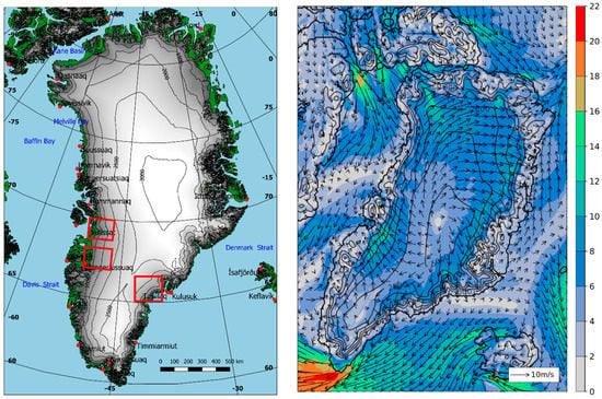
Figure 1.
Left: Map of Greenland with topography (isolines every 500 m). The red boxes mark the areas of the KABEG (Katabatic wind and boundary-layer front experiment around Greenland) experiment (shown in detail in Figure 2). Right: Topography (isolines every 500 m), 10 m wind speed (color shaded, in m/s), and 10 m wind vectors (every fifth grid point, scale in the lower right corner) of a CCLM simulation valid at 06:00 UTC 22 April 1997.
Data on the katabatic wind structure over the Greenland ice sheet are rare, particularly for wintertime conditions (no surface melting). Profile measurements of the katabatic wind over the West Greenland ice sheet were shown by [3] for a summertime situation during the Greenland Ice Margin Experiment (GIMEX) [4]. In the same area, the aircraft-based experiment KABEG (Katabatic wind and boundary-layer front experiment around Greenland) was performed in April/May 1997 [5]. Studies of the boundary-layer dynamics based on aircraft profiles yielded the results that the katabatic flow was always shooting (Froude number larger than 1) and that the katabatic force is the main driving mechanism for the flow regime [5]. The KABEG data represent a unique data set, since high-resolution profiles (a few meters vertically, approximately 5 km horizontally) for eight katabatic wind situations allow for a detailed picture of the katabatic wind structure along the slope. KABEG data have been used for the verification of weather forecast models in the past [6,7,8], but not for current regional climate models (RCMs) that are used, e.g., in the frame of Arctic Co-Ordinated Regional Downscaling Experiment (Arctic CORDEX) [9]. Recent comparisons between European Centre for Medium-Range Weather Forecasts (ECMWF) reanalyses [10], Arctic System reanalysis (ASR, [11]), and the COSMO-CLM regional climate model [12] have shown the largest differences for 10 m wind over the slopes of Greenland, i.e., the katabatic wind regions. On the other hand, verifications of the Regional Atmospheric Climate Model (RACMO) [13] using automatic weather station (AWS) data for Greenland show only a very small bias for the near-surface wind speed. Since katabatic wind is typically associated with a low-level jet (LLJ) near the top of the SBL [14,15], the vertical structure of the katabatic wind is of importance for the exchange between the surface and the free atmosphere.
2. Experimental Data and Model Description
2.1. The KABEG Experiment
The aircraft-based experiment KABEG was performed during April/May 1997 in the area of South Greenland (Figure 1). The main goals were the investigation of boundary-layer fronts over the Davis Strait [16] and the katabatic wind under high-pressure conditions [5]. In the present paper, only data of the katabatic wind flights are used. The aircraft was based at Kangerlussuaq, and area K1 close to Kangerlussuaq was the main investigation area (Figure 2). In this area, automatic weather stations (AWSs) were installed along a line oriented parallel to the fall line (Figure 3a): two surface energy balance stations over the ice (A3 and A4, measuring temperature and wind profiles, snow temperature profiles, and net radiation) and two wind recorders (A1 and A2). In addition, one AWS (U2 in Figure 3a) operated by the University of Utrecht (IMAU) is also located in area K1 (see [5] for detailed documentation). Six flights were performed in area K1 (see Table 1). Area K2 is at the eastern part of Greenland near Tasiilaq/Kulusuk, where pronounced valley structures with steep topographic gradients are present (Figure 3b). Area K3 is near Ilulissat over the Ilulissat glacier. Two AWSs (Swiss Camp and JAR1) of the Greenland Climate Network (GC-NET, [17]) lie inside the K3 area (Figure 3c).
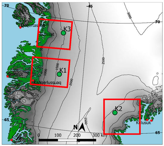
Figure 2.
Map of Greenland with topography (isolines every 500 m). The red boxes mark the areas of the KABEG experiment: K1 near Kangerlussuaq, K2 near Kulusuk, and K3 near Ilulissat. The green dots are the positions for the comparisons of vertical profiles.
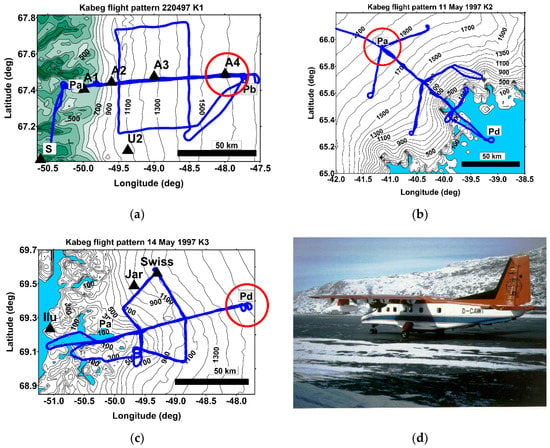
Figure 3.
Detailed maps of the areas of the KABEG experiment (see Figure 2) with superimposed flight tracks with reference points. (a) area K1, (b) area K2, (c) area K3. The red circles mark the positions for comparisons of vertical profiles (A4 for K1, Pa for K2, and Pd for K3). The black triangles mark positions with meteorological measurements. A picture of the aircraft POLAR2 is shown in panel (d).

Table 1.
KABEG flights and positions used for comparison with CCLM for April and May 1997.
The aircraft used was the research aircraft POLAR2 (Dornier 228, Figure 3d) owned by the Alfred Wegener Institute (Bremerhaven, Germany). The GPS-navigated aircraft measured position, wind vector, air temperature, and humidity via several instruments with sampling rates between 12 and 120 Hz (see [5] for details). The aircraft data used in this study are vertical profiles flown as slantwise aircraft profiles (ascents or descents). The horizontal distance of two consecutive vertical profiles is about 5 km. For comparison with simulations, locations in relatively homogeneous terrain were selected. These positions are marked in Figure 2 and Figure 3, and coordinates are given in Table 1. Since the aircraft data have a vertical resolution of a few meters, consecutive aircraft profiles around these positions were averaged in vertical bins of 10 m for the lowest 200 m and 20 m for between 200 m and 340 m. These horizontally and vertically averaged boundary-layer profiles are more appropriate for intercomparisons with model data.
Katabatic wind flights were performed on eight days (Table 1). For the six flights in area K1 (KA1–6, KA8), the profiles were flown at two different times (P1 and P2 in Table 1). In all flights, an LLJ was measured. For KA2 and KA4, the jet maximum was not fully covered by the aircraft profile, since the LLJ was too low (the lowest height of the aircraft was 30 m).
2.2. The CCLM Model
The regional climate model COSMO-CLM (CCLM, [18]) is the community model of the German regional climate research community. For the present paper, CCLM was used with a horizontal resolution of 15 km for the whole Arctic (Figure 4), and it covers the domain of Arctic CORDEX [19]. Initial and boundary data were taken from ERA-Interim reanalyses [10] with six-hourly resolution (ERA5 data [20] were not available when the simulations were performed). The model was used in daily forecast mode (spin-up time of 6 h) for the months of April and May 1997 (the KABEG period). Model output was available every 1 h. In the vertical, the model extends up to 22 km with 60 vertical levels; 12 of these levels are below 500 m in order to obtain a high resolution of the boundary layer. The sea ice concentration as shown in Figure 4 was taken from [21]. Topography data were taken from [22]. Full technical documentation of the CCLM model can be found in [23]. The modifications for the Arctic are described in the literature [12,24,25].
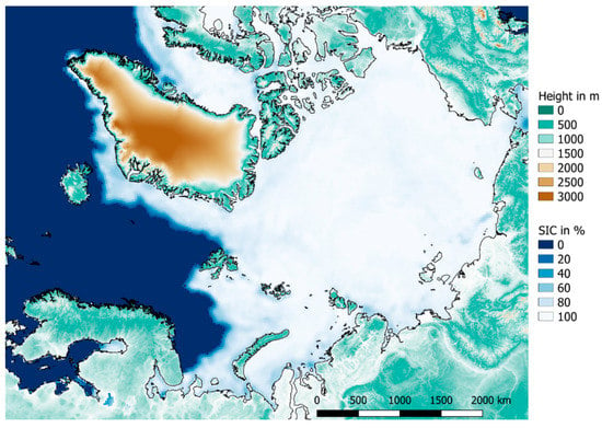
Figure 4.
Domain of the CCLM 15 km model domain with topography and sea ice concentration (SIC) for 22 April 1997.
Of particular interest for the present study are changes in the parameterization of turbulence in the stable boundary layer compared to the standard version of CCLM. For the very stable boundary layer over the Antarctic ice sheet, [26] found that CCLM strongly underestimates the strength of the surface inversion, which leads to a warm bias for the near-surface temperature over the Antarctic plateau. The main reason was that in the standard turbulence parameterization [23], the diffusion coefficients for heat and momentum are restricted to a minimal value of 0.4 m²/s. The use of minimum diffusion coefficients is common in operational weather forecast models. The motivation is to avoid too-low temperatures near the surface during the nighttime SBL with very weak winds [27]. In operational configurations of the turbulence scheme used for numerical weather prediction via the COSMO model by several national meteorological services, even higher values of 1.0 m²/s are used [27]. While the turbulent fluxes at the surface are computed by the scheme of [28], the diffusion coefficients are used for the parameterization of turbulent transports within the atmospheric boundary layer (ABL). The diffusion coefficients are computed by using the turbulent kinetic energy (TKE). CCLM uses a prognostic TKE scheme (1.5-order turbulence closure at level 2.5 [29]), where turbulent fluxes and transport terms are calculated from the diffusion coefficients and the respective gradients (see [23] for a full description). In addition, the standard CCLM uses parameterization for the generation of TKE by subgrid eddies via a thermal circulation term in the TKE equation [30], which increases the TKE production, particularly in the SBL. The authors of [30] and [27] concluded that the minimum turbulent diffusion coefficients and the thermal circulation term need to be reduced for simulations of the SBL. The authors of [27] recommend a minimal value of 0.01 m²/s, which is the same value as that used in an earlier version of the CCLM model by [31]. Souverijns et al. [32] used CCLM for the Antarctic with a minimal value of 0.03 m²/s and set the thermal circulation term to a very small value. The authors of [26] used a minimal value of 0.01 m²/s and neglected the thermal circulation term completely (as in [30]). In the following, the CCLM runs using the standard parameterizations are referred to as “default” (def), while the runs with parameterizations as used by [26] are referred to as “modified” (mod).
3. Results
3.1. CCLM Simulations for Greenland
In order to show the overall effect of the modified turbulence parameterization, Figure 5 shows the difference (mod–def) as the monthly average for April 1997 for the 2 m temperature and the 10 m wind speed. While the temperature over sea ice and ocean areas is almost unchanged, the run using the modified turbulence parameterization leads to up to 4 K lower temperatures over the Greenlandic ice sheet. The differences are largest over northern Greenland for elevations larger than 1000 m, while the changes over the slopes are around 1–2 K. The impact on the wind is small, but a general small increase of katabatic wind over the slopes of about 1 m/s can be seen. These findings agree with the results of [26] for the Antarctic for a long-year run, where a decrease of 7 K was simulated for the plateau during winter, while changes in the katabatic wind areas and over the sea ice were relatively small.
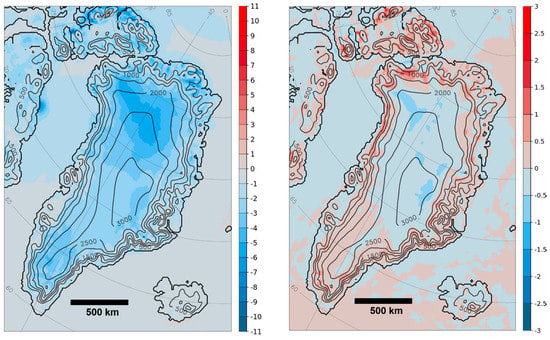
Figure 5.
Difference between runs using the different turbulence parameterizations (mod–def) as the monthly average for April 1997 for the 2 m temperature (in K, left) and the 10 m wind speed (in m/s, right).
3.2. Comparison with KABEG AWS Data
AWS measurements of KABEG station A4 were used for this comparison. A4 is located over the relatively homogeneous interior part of the ice sheet at a height of 1600 m (the height of the model grid point used for comparison is 1550 m). The time series for the full KABEG period from 16 April to 17 May 1997 is shown in Figure 6. The AWS data show a pronounced daily course of the temperature for almost all days, while the wind has a daily cycle only for periods with weak synoptic forcing (e.g., 26 April to 2 May 1997). The authors of [33] found a peak to peak amplitude of up to 5 m/s for the daily course of the wind speed during weak synoptic forcing. The strongest winds occur during strong synoptic forcing, e.g., for 21 April 1997 (flight KA2, see Table 1) and 22 April 1997 (flight KA3). Both simulations (def and mod) reproduced the near-surface wind speed for the whole period very well (Figure 6). For the temperature, the runs with the modified turbulence scheme reproduced the nighttime minima and the daily course better than the def run (see Table 2 for the overall statistics). This is illustrated more clearly in Figure 7 for the period 20–22 April 1997, where the mod run agrees almost perfectly with the AWS data, while the def run is too warm and shows a much weaker temperature amplitude. The near-surface wind speed and direction were simulated well by both model versions and were dominated by strong synoptic forcing.
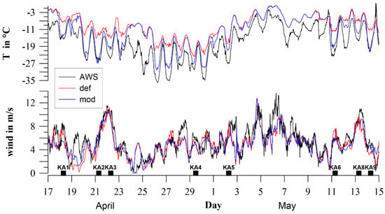
Figure 6.
Temperature (upper panel) and wind speed (lower panel) for the period 17 April to 15 May 1997 for automatic weather station (AWS) A4 (15 min values, black), the standard turbulence parameterization (def, red), and the modified turbulence parameterization (mod, blue). Wind and temperature for the AWS were taken at 2 m height; the simulated data are the 2 m temperature and the 10 m wind (hourly values). Black squares mark the times of the katabatic wind flights.

Table 2.
Comparison of CCLM simulations (sim) with AWS A4 for April and May 1997 for temperature and wind speed (RMSE: root mean square error, corr: correlation; AA: daily temperature amplitude, def: standard turbulence parameterization, mod: modified turbulence parameterization).
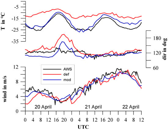
Figure 7.
Temperature (upper panel), wind direction (middle panel) and wind speed (lower panel) for the period 00:00 UTC 20 April 1997 to 12:00 UTC 22 April 1997 for AWS A4 (15 min values, black), the standard turbulence parameterization (def, red), and the modified turbulence parameterization (mod, blue).
Figure 8 shows the surface fluxes of net radiation (Q0) and sensible heat flux (H0) for the period 20–22 April 1997. The daily cycle of the net radiation was simulated well by both model runs, but the mod run is closer to the observations, particularly for the period with strong negative Q0 on 22 April. This is mainly a result of the stronger emission in the def run because of the higher temperature (the shortwave radiation balance was identical for both runs). Larger differences were found for the sensible heat flux. For the AWS, the turbulent fluxes were computed from the profiles of wind and temperature measured at three levels (0.3, 0.8, and 1.9 m) using the similarity theory (for details, see [33]). The def run strongly overestimated the (negative) sensible heat flux during the night, while the mod run agrees better with the measurements.
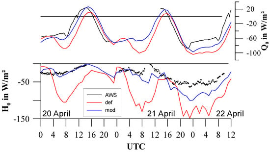
Figure 8.
Net radiation (Q0) and sensible heat flux (H0) for the period 00:00 UTC 20 April 1997 to 12:00 UTC 22 April 1997 for AWS A4 (15 min values, black), the standard turbulence parameterization (def, red), and the modified turbulence parameterization (mod, blue).
The overall statistics of the comparison with A4 wind and temperature data are presented in Table 2. For this comparison, AWS data were used as hourly values, and data were linearly detrended for the calculation of correlations. The bias in wind speed is very small for both model versions, and the root mean square error (RMSE) and correlations are almost the same. The differences for the temperature are larger. The bias is reduced by 2.5 K for the mod version, and the RMSE is reduced by more than 2 K. In order to quantify the daily amplitude, the AWS and model time series were low-pass filtered using a Gaussian filter with a filter width of 36 h. The daily variations were calculated by subtraction of the low-pass-filtered time series from the original time series. As a measure of the mean daily amplitude, the difference between the 90% and 10% percentiles of the daily variations was calculated. This average amplitude is almost 5 K larger than for the def run and agrees very well with the AWS data (Table 2).
3.3. Comparison with KABEG Aircraft Profiles
3.3.1. Case Study
The flight KA3 on 22 April 1997 was selected for this case study. The 10 m wind field simulated by CCLM (mod) for 06:00 UTC 22 April is shown in Figure 1. Strong katabatic winds with wind speeds of more than 10 m/s are present over the slopes of area K1. Good agreement with the AWS data was shown in the last section. The aircraft profiles P1 at location A4 on 22 April 1997 were flown at about 07:40 UTC (see Table 1). The CCLM simulations started at 18:00 UTC on 21 April. The simulated profiles shown are valid at 08:00 UTC (Figure 9) and 06:00 UTC (Figure 10). The aircraft profile shows a well-defined low-level jet (LLJ) at around 90 m height. The LLJ is associated with strong directional shear from 130° at low levels to southerly directions above the LLJ. The SBL is well developed, with coldest temperatures below 100 m. A similar structure can be seen in the humidity profile. The def run at the time of the observation (Figure 9) does not capture the observed temperature and humidity structure. A very broad wind maximum with much less vertical shear in speed and direction was simulated. In the mod run at 08:00 UTC, the temperature and humidity structure, as well as the directional shear, were simulated in a more realistic way. The representation of the LLJ structure is improved, but wind speeds are much lower than the observations. Taking the mod run at 06:00 UTC (Figure 10) leads to an LLJ with almost the right wind speed, but at a slightly greater height. No improvement can be seen for the def run at 06:00 UTC when compared to 08:00 UTC. The decrease in the strength of the LLJ can be seen also in the aircraft profile P2 flown at 11:00 UTC, which shows the LLJ speed to be about 5 m/s lower than for P1 (Table 1). The aircraft-measured profiles of the turbulent diffusion coefficients around the A4 position for flight P1 on 22 April 1997 (see Appendix A, Figure A1) show that with the exception of the lowest level, all coefficients are smaller than the threshold of 0.4 m² s−1 used in the def run. These low values for the turbulent diffusion coefficients are typical for the katabatic wind (Appendix A, Figure A2). This case study shows that although the wind comparison with AWS data at ground level shows good agreement for the def run, the development of the LLJ maximum might still not be captured well.
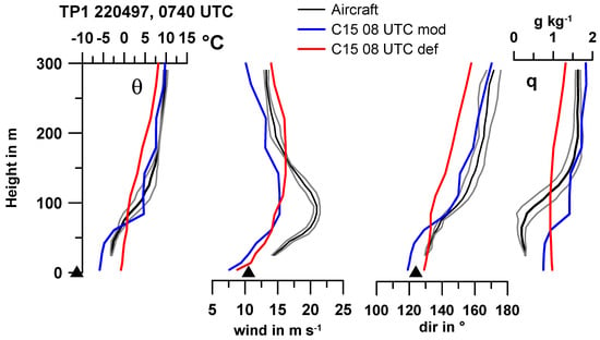
Figure 9.
Averaged aircraft profiles for 07:40 UTC (black line) and simulations (def: red, mod: blue) for 08:00 UTC 22 April 1997 for profile P1 (see Table 1). The grey lines associated with the aircraft data show the standard deviation of the data in the vertical bins. The displayed variables are potential temperature (θ), wind speed, wind direction, and specific humidity (q). The data of AWS A4 at 07:45 UTC are shown as triangles.
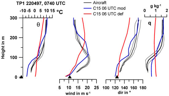
Figure 10.
Averaged aircraft profiles for 07:40 UTC (black line) and simulations (def: red, mod: blue) for 06:00 UTC 22 April 1997 for profile P1 (see Table 1). The grey lines associated with the aircraft data show the standard deviation of the data in the vertical bins. The displayed variables are potential temperature (θ), wind speed, wind direction, and specific humidity (q). The data of AWS A4 at 07:45 UTC are shown as triangles.
The case of 22 April 1997 represents a situation with strong synoptic forcing. The simulations show an SBL throughout the day resulting in a permanent katabatic force. The hodograph from the mod simulation at 140 m (height of the simulated LLJ) and at 270 m (Appendix A, Figure A3) shows that the decay of the LLJ is associated with decaying synoptic forcing. The analysis of the forces on the katabatic flow for the P1 profile by [5] showed that the synoptic forcing term is about 60% of the katabatic forcing term. Different behavior of the flow development can be seen for a case with medium synoptic forcing on 2 May 1997 (Appendix A, Figure A3).
3.3.2. ABL Statistics
Statistics of the comparisons of simulations with aircraft profiles were computed for all KABEG flights for wind speed below 350 m (Figure 11). The times of comparisons (as documented in Table 1) were chosen within a time window of about two hours around the time of the observation. For the bias, no improvement for the mod run can be seen, which results from the fact that even if the LLJ is not simulated at all by the def run, the wind speed underestimation in the lower part of the SBL is compensated by an overestimation in the upper part (see Figure 10). For the RMSE, an overall improvement for the mod run was found. The general better representation of the wind structure for the mod run is documented by the correlations (without detrending). For most profiles, the mod run shows correlations larger than 70%, while the def run shows weak or even negative correlations in most cases.
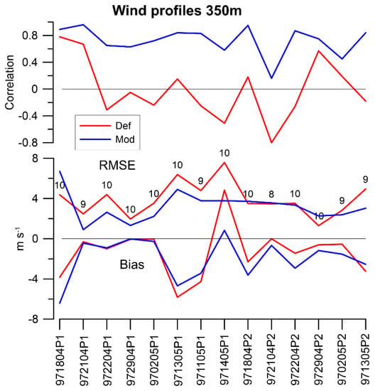
Figure 11.
Statistics of the comparisons of simulations (def: red, mod: blue) with aircraft profiles for all KABEG flights for wind speed below 350 m (x axis: date (YYDDMM) and profile (P1/P2)). Lower panel: Bias and RMSE (number of values indicated). Upper panel: Correlation.
In order to quantify the representation of the SBL structure in more detail, different gradients were computed for the simulations and aircraft profiles. An LLJ was observed in all KABEG flights (see Table 1). The SBL in the lowest 200 m is typically associated with distinct shear in wind direction and inversion (see Figure 10). The gradients of the potential temperature and wind direction were therefore computed for the lowest 200 m. In order to characterize the wind increase below and the wind decrease above the LLJ maximum, wind speed gradients were computed within 100 m above (as detected by the aircraft measurements) and below the LLJ, if the wind maximum was at least 40 m above the lowest height of the aircraft profile. For four profiles, the LLJ was too low to pass the latter criterion.
The gradients of the potential temperature and wind direction in the ABL (Figure 12) were generally much better simulated in the mod run than in the def run (see individual profiles and the average). A strong improvement for the mod run in representing the LLJ structure can be seen for the wind gradient above the LLJ (Figure 13a). In the average, the def run shows an opposite sign compared to the measurements, i.e., an increase in wind speed was simulated instead of a decrease. For wind gradient below the LLJ, the simulations show over- and underestimations, and no improvement by the mod run can be seen. A main difference between the two model runs and the observations is also the height of the LLJ (Figure 14), which was generally simulated at too-large heights in the def run, while the mod run shows much better agreement. When the wind speed gradients were calculated by taking LLJ heights individually from observations and from each simulation, the improvement for the mod run was even better (Figure 13b).
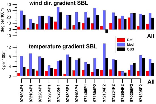
Figure 12.
Gradients in the ABL from aircraft profiles (black) and simulations (def: red, mod: blue) for all KABEG flights (see Table 1) and as an average for all profiles (All). Upper panel: Wind direction gradient in the lowest 200 m. Lower panel: Potential temperature gradient in the lowest 200 m (all values per 100 m). x axis as in Figure 11.
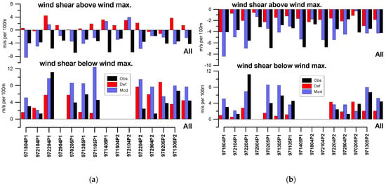
Figure 13.
(a) Wind speed gradients (all values per 100 m) from aircraft profiles (black) and simulations (def: red, mod: blue) for all KABEG flights (see Table 1) and as an average for all profiles (All). Upper panel: Gradients within 100 m above the observed low-level jet (LLJ), Lower panel: Gradients below the LLJ. (b) As Figure 13a, but for wind speed gradients taking LLJ heights individually from observations and from each simulation (see Figure 14 for LLJ heights).
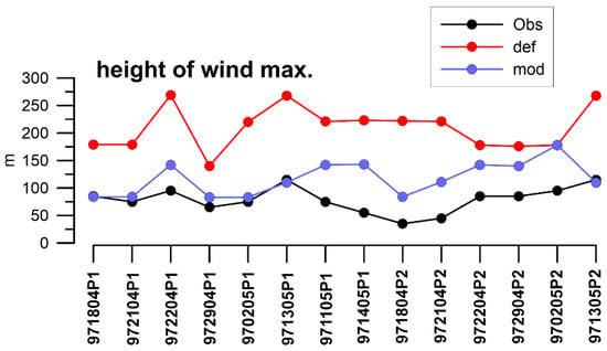
Figure 14.
Height of the wind maximum from aircraft profiles (black) and simulations (def: red, mod: blue) for all KABEG flights (see Table 1).
4. Discussion
There have been only few verification studies of the katabatic wind structure over the Greenland ice sheet. The main reason for this is that data sets of in situ or remote sensing measurements of the katabatic wind over the slopes of the ice sheet are rare. For the Antarctic, the authors of [34] measured wind profiles on 28 days over a slope south of Halley station using a Doppler sodar. They found LLJs at relatively low levels (below 60 m) and of medium strength (maximum winds of 8–10 m s−1), which were compared to idealized model simulations. The authors of [35] compared different SBL parameterizations of a 1D version of a global climate model with measurements of a 45 m tower over the Antarctic plateau. Here, the lack of topography gradients prevented the development of katabatic flows, but verifications could be performed for the very stable boundary layer during weak wind conditions.
In most verification studies on the boundary layer over the Greenland ice sheet, only near-surface AWS data were used for the verification (e.g., [13,36]). The KABEG data set is one of the most comprehensive data sets for the study of the structure of katabatic winds. Katabatic wind is typically associated with a fully turbulent SBL and a strong LLJ (up to 22 m s−1) near the top of the SBL [14,15]. Besides the strength and height of the LLJ, mesoscale katabatic winds differ from weaker slope winds in terms of the turbulence structure [37]. While studies of the turbulence in slope winds (e.g., [38]) show increasing TKE above the wind maximum, no or weak turbulence is found for deeper mesoscale katabatic flows [37]. This behavior of the TKE structure was also found for the KABEG cases [14] and is explained by the fact that the LLJ is embedded within the inversion [37].
Comparisons of KABEG profiles with the polar Mesoscale Meteorology Model 5 (MM5) [6], the Norwegian Limited Area model (NORLAM) [8], and the Lokal-Modell (LM) model [7] have shown that these models could reproduce the katabatic SBL relatively well, but deficits in the representation of physical processes in the SBL were found as well [6]. There has been fast development of regional climate models (RCMs) in the last two decades, and it is expected that these developments have led to improvements in the simulations. Recent comparisons of current regional climate models (including CCLM) with measurements over the Arctic ocean [9] have shown good quality of the simulations, but no large improvements compared to former RCM generations (e.g., [39]) were found. The authors of [26] showed that modification of the turbulence scheme in CCLM for the SBL yielded a better representation of the near-surface temperature and the SBL structure over the Antarctic plateau with relatively weak winds. No verification could be made for the katabatic wind region to show whether the modified parameterizations also yielded improved representation of the katabatic wind structure. The present study shows that deficits in SBL parameterization, even under conditions of strong winds, are present in the default parameterization of CCLM. A comparison of diffusion coefficients measured during KABEG with the 0.4 m² s−1 threshold for minimal diffusion coefficients used by the default parameterization showed that 95% of the kH values and 68% of the km values were lower than this threshold (Appendix A, Figure A2). Thus, the use of minimum diffusion coefficients, as in the operational configurations of weather forecast models, is not applicable for the SBL in situations with enough shear-generated turbulence [27], which is found over ice sheets [40] and particularly in katabatic winds.
The comparison with an automatic weather station (AWS) installed during KABEG (during April and May 1997) showed that the change in near-surface wind speed by the modified parameterizations (mod) is very small. In contrast, the simulations of daily temperature variations were largely improved in the mod runs. In addition, the sensible heat flux came close to the measured values.
The mod runs yielded a generally better representation of the wind, temperature, and moisture structure. In particular, the LLJ structure was simulated much better than in the def run, where the wind speed maximum was almost not present and the turning of the wind with height was largely underestimated. As in [6,8], a time shift of up to about 2 h was found between the time of the aircraft observation and the time of the best simulated profile. This indicates that correct simulation of the synoptic setting is also of high importance.
The KABEG profiles used in this study will be published in a database and can be used as a benchmark for other regional climate models.
5. Conclusions
The state-of-the-art RCM CCLM was evaluated for the representation of the katabatic wind structure over Greenland using the standard turbulence parameterization and a modified parameterization for the SBL allowing for a better representation of the surface inversion over polar ice sheets during weak wind conditions [26]. The main conclusions from this study are as follows:
- The modified parameterization (mod) yielded slightly higher katabatic winds near the surface for the monthly means of April and May 1997. The near-surface temperature in the katabatic wind regions was slightly colder.
- Comparison with an AWS for April and May 1997 showed much better simulation of the daily course of the temperature and the sensible heat flux for the mod run.
- Comparison with aircraft profiles showed that the mod run yielded more realistic profiles, particularly a better representation of the LLJ.
Overall, the improvements in the SBL parameterization, designed for better representation of the very stable boundary layer during weak wind conditions, also yielded better simulation of the katabatic wind structure, i.e., even for strong wind conditions. Since katabatic wind is a quasi-permanent system over polar ice sheets, and since it is of large importance for exchange between the surface and the free atmosphere, the representation of the katabatic SBL in state-of-the-art RCMs and in reanalyses [11,20] should be checked.
Funding
This research was partly funded by the Federal Ministry of Education and Research (BMBF) under grants 03F0776D and 03F0831C in the frame of German–Russian cooperation “WTZ RUS: Changing Arctic Transpolar System (CATS)”. The publication was funded by the Open Access Fund of the University of Trier and the German Research Foundation (DFG) within the Open Access Publishing funding programme.
Acknowledgments
Thanks go to Lukas Schefczyk (Environmental Meteorology, University of Trier) for performing the CCLM simulations. The author thanks the CLM Community and the German Meteorological Service for providing the basic COSMO-CLM model. The DKRZ (Hamburg) is acknowledged for providing computation time.
Conflicts of Interest
The author declares no conflict of interest.
Data
The data will be made available on PANGAEA.
Appendix A
The KABEG turbulence data were evaluated in [14]. Figure A1 shows the profiles of the turbulent diffusion coefficients for heat (kH) and momentum (km) from aircraft data around the A4 position for flight P1 on 22 April 1997 (see Figure 9). The coefficients were derived from eddy covariance measurements of the turbulent fluxes and gradients of the mean quantities on flight segments of 8 km at different heights. Statistics of the turbulent diffusion coefficients for all K1 flights are shown in Figure A2. A comparison with the 0.4 m² s−1 threshold for the minimal diffusion coefficients used by the default parameterization shows that 95% of the kH values and 68% of the km values are lower than this threshold, while 38% of the kH values and 18% of the km values are lower than 0.05 m² s−1.
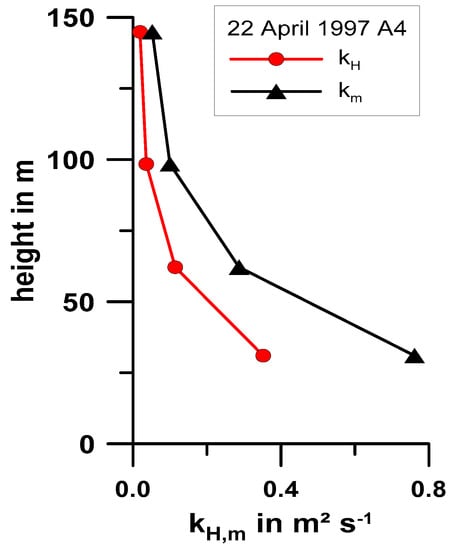
Figure A1.
Profiles of the turbulent diffusion coefficients for heat (kH) and momentum (km) from aircraft data around the A4 position for flight P1 on 22 April 1997.
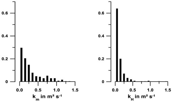
Figure A2.
Relative frequency distribution of the turbulent diffusion coefficients for heat (kH) and momentum (km) from aircraft data for all K1 flights (total number of values: 247; bins of 0.1 m² s−1).
Hodographs from simulations at two heights are shown in Figure A3 for a case with strong synoptic forcing (22 April 1997) and a case with medium synoptic forcing (2 May 1997). For both cases, the lower height is approximately at the height of the observed LLJ (see Figure 14), and the upper height can be regarded as free-atmosphere conditions. A negative u-component corresponds to a downslope wind. On 2 May, the downslope component at 85 m accelerated between 00 and 09 UTC (local midnight is around 03:00 UTC), while the flow at 180 m was almost constant from southerly directions. On 22 April 1997, the downslope component at 140 m decelerated between 00:00 and 10:00 UTC in a similar way to the flow at 270 m.
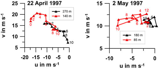
Figure A3.
Simulated hodographs (mod) for 00:00–10:00 UTC 22 April 1997 for heights of 140 m (red) and 270 m (black) and for 00:00–12:00 UTC 2 May (hourly values) for heights of 85 m (red) and 180 m (black). Labels are the time in UTC.
References
- Rasmussen, L. Greenland Winds and Satellite Imagery. Vejret Dan. Meteorol. Soc. 1989, 32–37. [Google Scholar]
- Heinemann, G.; Klein, T. Modelling and observations of the katabatic flow dynamics over Greenland. Tellus A Dyn. Meteorol. Oceanogr. 2002, 54, 542–554. [Google Scholar] [CrossRef]
- Van den Broeke, M.R.; Duynkerke, P.G.; Henneken, E.A.C. Heat, momentum and moisture budgets of the katabatic layer over the melting zone of the west Greenland ice sheet in summer. Bound. Layer Meteorol. 1994, 71, 393–413. [Google Scholar] [CrossRef]
- Oerlemans, J.; Vugts, H.F. A Meteorological Experiment in the Melting Zone of the Greenland Ice Sheet. Bull. Am. Meteor. Soc. 1993, 74, 355–365. [Google Scholar] [CrossRef]
- Heinemann, G. The KABEG’97 field experiment: An aircraft-based study of katabatic wind dynamics over the Greenland ice sheet. Bound. Layer Meteorol. 1999, 93, 75–116. [Google Scholar] [CrossRef]
- Bromwich, D.H.; Cassano, J.J.; Klein, T.; Heinemann, G.; Hines, K.M.; Steffen, K.; Box, J.E. Mesoscale Modeling of Katabatic Winds over Greenland with the Polar MM5*. Mon. Weather Rev. 2001, 129, 2290–2309. [Google Scholar] [CrossRef]
- Klein, T.; Heinemann, G.; Gross, P. Simulation of the katabatic flow near the Greenland ice margin using a high-resolution nonhydrostatic model. Meteorol. Z. 2001, 10, 331–339. [Google Scholar] [CrossRef]
- Klein, T.; Heinemann, G.; Bromwich, D.H.; Cassano, J.J.; Hines, K.M. Mesoscale modeling of katabatic winds over Greenland and comparisons with AWS and aircraft data. Meteorol. Atmos. Phys. 2001, 78, 115–132. [Google Scholar] [CrossRef][Green Version]
- Sedlar, J.; Tjernström, M.; Rinke, A.; Orr, A.; Cassano, J.; Fettweis, X.; Heinemann, G.; Seefeldt, M.; Solomon, A.; Matthes, H.; et al. Confronting Arctic troposphere, clouds, and surface energy budget representations in regional climate models with observations. J. Geophys. Res. 2020. [Google Scholar] [CrossRef]
- Dee, D.P.; Uppala, S.M.; Simmons, A.J.; Berrisford, P.; Poli, P.; Kobayashi, S.; Andrae, U.; Balmaseda, M.A.; Balsamo, G.; Bauer, P.; et al. The ERA-Interim reanalysis: Configuration and performance of the data assimilation system. Q. J. R. Meteorol. Soc. 2011, 137, 553–597. [Google Scholar] [CrossRef]
- Bromwich, D.H.; Wilson, A.B.; Bai, L.; Liu, Z.; Barlage, M.; Shih, C.-F.; Maldonado, S.; Hines, K.M.; Wang, S.-H.; Woollen, J.; et al. The Arctic System Reanalysis, Version 2. Bull. Am. Meteor. Soc. 2018, 99, 805–828. [Google Scholar] [CrossRef]
- Gutjahr, O.; Heinemann, G. A model-based comparison of extreme winds in the Arctic and around Greenland. Int. J. Clim. 2018, 38, 5272–5292. [Google Scholar] [CrossRef]
- Ettema, J.; van den Broeke, M.R.; van Meijgaard, E.; van de Berg, W.J.; Box, J.E.; Steffen, K. Climate of the Greenland ice sheet using a high-resolution climate model–Part 1: Evaluation. Cryosphere 2010, 4, 511–527. [Google Scholar] [CrossRef]
- Heinemann, G. Aircraft-Based Measurements of Turbulence Structures in The Katabatic Flow Over Greenland. Bound. Layer Meteorol. 2002, 103, 49–81. [Google Scholar] [CrossRef]
- Heinemann, G. Local Similarity Properties of the Continuously Turbulent Stable Boundary Layer over Greenland. Bound. Layer Meteorol. 2004, 112, 283–305. [Google Scholar] [CrossRef]
- Drüe, C.; Heinemann, G. Airborne Investigation of Arctic Boundary-Layer Fronts over the Marginal Ice Zone of the Davis Strait. Bound. Layer Meteorol. 2001, 101, 261–292. [Google Scholar] [CrossRef]
- Steffen, K.; Box, J.E.; Abdalati, W. Greenland Climate Network: GC-Net. US Army Cold Reg. Reatt. Eng. 1996, 98–103. [Google Scholar]
- Rockel, B.; Will, A.; Hense, A. The Regional Climate Model COSMO-CLM (CCLM). Meteorol. Z. 2008, 17, 347–348. [Google Scholar] [CrossRef]
- Akperov, M.; Rinke, A.; Mokhov, I.I.; Matthes, H.; Semenov, V.A.; Adakudlu, M.; Cassano, J.; Christensen, J.H.; Dembitskaya, M.A.; Dethloff, K.; et al. Cyclone Activity in the Arctic From an Ensemble of Regional Climate Models (Arctic CORDEX). J. Geophys. Res. 2018, 123, 2537–2554. [Google Scholar] [CrossRef]
- Hersbach, H.; de Rosnay, P.; Bell, B.; Schepers, D.; Simmons, A.; Soci, C.; Abdalla, S.; Alonso-Balmaseda, M.; Balsamo, G.; Bechtold, P.; et al. Operational Global Reanalysis: Progress, Future Directions and Synergies with NWP; European Centre for Medium Range Weather Forecasts: Reading, UK, 2018. [Google Scholar]
- OSI SAF. Global Sea Ice Concentration Climate Data Record v2.0-Multimission; EUMETSAT: Darmstadt, Germany, 2017. [Google Scholar]
- Hastings, D.A.; Dunbar, P.K. Global Land One-kilometer Base Elevation (GLOBE) Digital Elevation Model, Documentation. Natl. Ocean. Atmos. Adm. 1999, 325, 80305–83328. [Google Scholar]
- Zentek, R. COSMO Documentation (Archived Version from 2019, Uploaded with Permission of the DWD). 2019. Available online: https://zenodo.org/record/3339384 (accessed on 13 May 2020).
- Gutjahr, O.; Heinemann, G.; Preußer, A.; Willmes, S.; Drüe, C. Quantification of ice production in Laptev Sea polynyas and its sensitivity to thin-ice parameterizations in a regional climate model. Cryosphere 2016, 10, 2999–3019. [Google Scholar] [CrossRef]
- Kohnemann, S.H.E.; Heinemann, G.; Bromwich, D.H.; Gutjahr, O. Extreme Warming in the Kara Sea and Barents Sea during the Winter Period 2000–16. J. Clim. 2017, 30, 8913–8927. [Google Scholar] [CrossRef]
- Zentek, R.; Heinemann, G. Verification of the regional atmospheric model CCLM v5.0 with conventional data and lidar measurements in Antarctica. Geosci. Model Dev. 2020, 13, 1809–1825. [Google Scholar] [CrossRef]
- Buzzi, M.; Rotach, M.W.; Raschendorfer, M.; Holtslag, A.A.M. Evaluation of the COSMO-SC turbulence scheme in a shear-driven stable boundary layer. Meteorol. Z. 2011, 20, 335–350. [Google Scholar] [CrossRef]
- Louis, J.-F. A parametric model of vertical eddy fluxes in the atmosphere. Bound. Layer Meteorol. 1979, 17, 187–202. [Google Scholar] [CrossRef]
- Mellor, G.L.; Yamada, T. A Hierarchy of Turbulence Closure Models for Planetary Boundary Layers. J. Atmos. Sci. 1974, 31, 1791–1806. [Google Scholar] [CrossRef]
- Cerenzia, I.; Tampieri, F.; Tesini, S. Diagnosis of Turbulence Schema in Stable Atmospheric Conditions and Sensitivity Tests. COSMO Newsl. 2014, 14, 1–11. [Google Scholar]
- Hebbinghaus, H.; Heinemann, G. LM simulations of the Greenland boundary layer, comparison with local measurements and SNOWPACK simulations of drifting snow. Cold Reg. Sci. Technol. 2006, 46, 36–51. [Google Scholar] [CrossRef]
- Souverijns, N.; Gossart, A.; Demuzere, M.; Lenaerts, J.T.M.; Medley, B.; Gorodetskaya, I.V.; Vanden Broucke, S.; van Lipzig, N.P.M. A New Regional Climate Model for POLAR-CORDEX: Evaluation of a 30-Year Hindcast with COSMO-CLM 2 Over Antarctica. J. Geophys. Res. 2019, 124, 1405–1427. [Google Scholar] [CrossRef]
- Heinemann, G.; Falk, U. Surface Winds and Energy Fluxes Near the Greenland Ice Margin under Conditions of Katabatic Winds. Polarforschung 2002, 71, 15–31. [Google Scholar]
- Renfrew, I.A.; Anderson, P.S. Profiles of katabatic flow in summer and winter over Coats Land, Antarctica. Q. J. R. Meteorol. Soc. 2006, 132, 779–802. [Google Scholar] [CrossRef]
- Vignon, E.; Hourdin, F.; Genthon, C.; Gallée, H.; Bazile, E.; Lefebvre, M.-P.; Madeleine, J.-B.; van de Wiel, B.J.H. Antarctic boundary layer parametrization in a general circulation model: 1-D simulations facing summer observations at Dome C. J. Geophys. Res. 2017, 122, 6818–6843. [Google Scholar] [CrossRef]
- Box, J.E.; Rinke, A. Evaluation of Greenland Ice Sheet Surface Climate in the HIRHAM Regional Climate Model Using Automatic Weather Station Data. J. Clim. 2003, 16, 1302–1319. [Google Scholar] [CrossRef]
- Stiperski, I.; Holtslag, A.A.M.; Lehner, M.; Hoch, S.W.; Whiteman, C.D. On the turbulence structure of deep katabatic flows on a gentle mesoscale slope. Q. J. R. Meteorol. Soc. 2020, 146, 1206–1231. [Google Scholar] [CrossRef]
- Grachev, A.A.; Leo, L.S.; Di Sabatino, S.; Fernando, H.J.S.; Pardyjak, E.R.; Fairall, C.W. Structure of Turbulence in Katabatic Flows Below and Above the Wind-Speed Maximum. Bound. Layer Meteorol. 2016, 159, 469–494. [Google Scholar] [CrossRef]
- Rinke, A.; Dethloff, K.; Cassano, J.J.; Christensen, J.H.; Curry, J.A.; Du, P.; Girard, E.; Haugen, J.-E.; Jacob, D.; Jones, C.G.; et al. Evaluation of an ensemble of Arctic regional climate models: Spatiotemporal fields during the SHEBA year. Clim. Dyn. 2006, 26, 459–472. [Google Scholar] [CrossRef]
- Drüe, C.; Heinemann, G. Characteristics of intermittent turbulence in the upper stable boundary layer over Greenland. Bound. Layer Meteorol. 2007, 124, 361–381. [Google Scholar] [CrossRef]
© 2020 by the author. Licensee MDPI, Basel, Switzerland. This article is an open access article distributed under the terms and conditions of the Creative Commons Attribution (CC BY) license (http://creativecommons.org/licenses/by/4.0/).