Initial Results of Meteor Wind with Langfang Medium Frequency Radar

Abstract

We conducted meteor observations during the Leonid meteor shower on 16 November 2017 and 17 November 2018 with Langfang medium frequency (MF) radar (116° E, 40° N). This was the first nighttime meteor observation by MF radar in mid-latitude China. The observation period was 12:00–22:00 (UT) and the observation range was 78–150 km. By using broad vertical beams, totally 94 and 92 meteor echoes were obtained, along with their spatial, time and height distribution. Quite a few meteor echoes are within 30° zenith angles, from the southwest direction, and with a mean height of 107 km which is almost 10 km higher than traditional VHF (Very High Frequency) meteor radar observations. Initial bi-hourly and nightly averaged wind profiles were calculated, and well fitted the wind estimations by co-located VHF meteor radar at the altitude of 100–110 km. On the other side, echoes around 140 km are successfully detected in our observation, which may suggest that for most running MF radars, meteor echoes around 140 km altitude could be detected with a sampling pulse frequency less than 100 Hz.

1. Introduction

Medium frequency (MF) radars operating at 1.5–3 MHz are powerful tools for obtaining wind field and electron density profiles from 60 to 100 km using techniques such as full correlation analysis (FCA) and differential absorption experiment (DAE) methods, which both have greatly contributed to short- and long-term atmospheric dynamic studies in the middle atmosphere [1,2,3]. However, due to the transmitting frequency, total reflection occurs at higher altitudes instead of partial reflection, which limits the wind detection height [4]. Additionally, the FCA method itself shows large discrepancies at altitudes greater than 100 km [5]. Therefore, it is difficult for conventional MF radars to make precise wind estimates above approximately 100 km, despite that this region has complicated dynamic changes and is of great significance.

Meteor radars are another measurement to derive winds in the mesosphere and lower thermosphere (MLT) region using meteor echoes [6,7]. However, most meteor echoes detected are concentrated at 90 km, resulting in low accuracy or data missing when calculating horizontal wind above 100 km. Therefore, MF radar measurement of meteor echoes may be another technique that enables horizontal wind detection at altitudes above 100 km. The relatively lower radio frequency of MF radar helps for detecting more meteor echoes than meteor radar in this region, which has been verified by Olsson-Steel and Elford that meteor echoes can exist up to 140 km altitude [8]. In addition, it has an advantage of compensating for the known problems of MF radar FCA techniques above around 90 km [5]. However, it should be noted here that the observation can only be conducted during nighttime, because total reflection occurs during the daytime, which severely obscures the meteor echoes. Additionally, MF radar is usually affected by local radio frequency interference, which has similar amplitude characteristics to meteor echoes.

There are about 50 MF radars established in the world, and some observations have been made to obtain horizontal wind over 100 km using meteor echoes from MF radars. For example, Meek and Manson, 1990, demonstrated the great potential MF radar has for meteor wind measurement [9]. Tsutsumi and Holdsworth, 1999, conducting meteor echo observations with the Buckland Park MF radar, obtained bi-hourly wind profiles at altitudes of 94–114 km [4]. Tsutsumi and Aso, 2005, presented the first long-term meteor observation results from the Syowa MF radar off the coast of Antarctica [10]. By comparing wintertime meteor and full correlation analysis wind observations, they obtained results that agreed well at approximately 90 km, whereas the FCA winds tended to underestimate the meteor winds at higher altitudes. Stephen, 2003, made extensive nighttime observations of both sporadic meteors and meteor shower events at an altitude of 70–160 km using the Buckland Park MF radar over a two-and-a-half-year period, and evaluated a variety of meteor wind measurement techniques [11]. Based on the experience of the above experiments, we adjusted some parameters in our MF radar meteor observations, such as pulse repetition frequency (PRF) and sampling range, so as to get better wind results.

In this paper, we report nighttime meteor observations with Langfang MF radar at altitudes greater than 100 km, which is the first time such observations have been conducted in mid-latitude China. Averaged horizontal wind profiles obtained by MF radar and co-located meteor radar are also compared for further analysis. Section 2 describes the principles of meteor wind measurements as a theoretical support for observational studies. Section 3 shows the meteor observation setup. We changed the PRF to 80 Hz, in order to investigate whether it is possible to detect meteor echoes with PRF less than 100Hz. Section 4 describes the data processing steps in meteor echo detection, and Section 5 presents meteor echo detection results, including spatial, time and height distribution, to prepare for the next wind calculation. Following this, the initial horizontal wind profiles from 96 km to 115 km and comparisons with co-located MF radar are shown in Section 6. The conclusions are presented in Section 7.

2. Principles of Meteor Wind Measurement

When meteoroids enter Earth’s atmosphere, they interact with atmospheric molecules, forming a long cylindrical meteor trail through the processes of evaporation and ionization [12,13]. Based on the electron density of meteor trials, meteor echoes can be divided into underdense echoes and overdense echoes. For overdense echoes, electron line density is typically greater than $2.4\times {10}^{14}{\pi }^3{(r_0/\lambda )}^2$ electrons per meter (where $r_0$ is the meteor trail’s initial radius and $\lambda$ is the radar wavelength) [14], thus secondary scattering becomes more significant and ambipolar diffusion of plasma trails would affect the Doppler frequency shift. In contrast, for underdense echoes, secondary scatter is weak and the total scattered radiation can be seen as the sum of individual electrons, showing strong echo phase coherence [15]. Therefore, underdense echoes rather than overdense echoes are usually picked up to calculate horizontal wind. Based on radar equations [11], receiving power under ideal conditions can be represented as

$$P_R=P_T{G}_T{G}_R{\lambda }^3{q}^2{r}_e^2\frac{C^2+S^2}{64{\pi }^2{R}_0^3}$$

(1)

where $P_T$, $G_T$ and $G_R$ are transmitting power, transmitting antenna gain and receiving antenna gain, respectively; $q$, and $r_e$ are the linear electron density of the trail and electron radius of meteor trails, respectively; $R_0$ is the minimum range between the radar and the meteor trail; and $C$ and $S$ are Fresnel integrals. According to Equation (1), the amplitude of basic meteor trail shows a sudden increase and following exponential decrease, and the phase is Doppler frequency shifted.

As a result of ambipolar diffusion, the meteor trail would expand in the radial direction after its formation [14,15]. As height increases in thermosphere, the background pressure varies exponentially and the increment is greater than the squared value of temperature, which accelerates the meteor echo decay process and shortens the trail duration (related formulas can be referred to in Appendix A). Thus, MF radars have advantages over VHF radars, namely long wavelength and duration, which helps obtaining atmospheric wind at altitudes greater than 100 km. However, there is a disadvantage in that meteor observations for MF radars can only be conducted at nighttime, as the E-region of ionosphere is highly ionized during the day, especially after sunrise, causing total reflection of radio waves.

Echo phase differences between receiving antennas can be used to estimate angle of arrival (AOA), including azimuth angle and zenith angle. Meteor trails drift with atmospheric wind, therefore radars receive a signal producing a Doppler shift, which can be expressed as

$$\Delta f=\frac{2\times v}{\lambda }$$

(2)

where v is the Doppler velocity along radar’s line of sight. Combined with the zenith and azimuth angles estimated from AOA, a two-dimensional decomposition of Doppler velocity in the horizontal direction can be used to obtain mesospheric neutral wind—assuming vertical velocity w is much smaller than the horizontal velocity and can thus be ignored [16,17,18]—as follows:

$$V=ul+vm$$

(3)

here, u and v are the zonal and meridional velocities, respectively, and l and m are the x and y components of the directional cosines estimated by AOA (x refers to the zonal direction and y refers to the meridional direction). In principle, horizontal wind can thus be obtained using two sufficiently spatially separated meteor echoes.

3. Experimental Setup of Meteor Observations

In May 2009, the National Space Science Center of the Chinese Academy of Sciences installed a relocatable MF radar at Langfang observatory. Its data has been used to analyze the atmospheric dynamics and electron density of the mesosphere and lower thermosphere [19,20]. This radar system consists of a transmitter, receiver, antennas and a data processing system. The spaced antenna array shown in Figure 1 consists of four orthogonal half-wave dipole antennas located at the vertices and center of an equilateral triangle with 181 m sides. The antennas are all used for transmission and reception. An equilateral triangle configuration reduces deviations in the wind field inversion process, and the minimum distance between any two antennas is 0.7 times the wavelength, effectively avoiding mutual coupling effects between antennas [21].

We conducted meteor observations with the Langfang MF radar during the night of 16 November 2017 and 17 November 2018, using the observational parameters listed in

Table 1. Langfang MF meteor observation parameters and VHF meteor radar parameters.

Parameter	MF Radar	VHF Meteor Radar
Frequency	1.99 MHz	35 MHz
Transmitting Power	64 kW	20 kW
Pulse Repetition Frequency	80 Hz	440 Hz
Height Resolution	2 km	2 km
Time Resolution (the length of individual time series)	2 min	1 h
Number of Coherent Integrations	2	16
Sampling Range	78–150 km	70–110 km
Polarization	O Mode	O Mode

. Earth’s magnetic field causes differences in radio wave propagation characteristics, such as ordinary mode (O mode) and extraordinary mode (E Mode), which are functions of polarization [10]. To avoid the strong ionospheric echoes in E mode, we chose O mode as the radar’s transmitting signal polarization mode. As a result that meteor detection requires a high sampling frequency and signal-to-noise ratio, we set the PRF and number of coherent integration points to 80 Hz and two, respectively, and set the sampling range to 78–150 km to avoid ionospheric interference and improve detection height.

We also collected meteor wind using co-located VHF meteor radar, which usually obtains meteor echoes at altitude of 70–110 km with 2 km height resolution and 1 hour time resolution [22,23]. The parameters are listed in Table 1. We later compared meteor wind over 100–110 km of the two radars to verify the feasibility of MF meteor wind measurement techniques.

4. Meteor Echo Detection and Data Analysis

Meteor echo detection is a difficult task, which is performed using two successive steps: preliminary detection and confirmation of suspected meteor echoes. Parameter estimation is then performed to calculate meteor height, AOA and radial drifted velocity. The atmospheric wind profile is thus finally obtained using the above parameters.

4.1. Detection Algorithms

Langfang MF radar is usually affected by local RF interference, which has similar amplitude characteristics to meteor echoes; therefore, preprocessing the received raw data is the first step toward improving the signal-to-noise ratio and weakening interference. First, we reduced the sampling rate to 10 Hz by coherently integrating the original data from four receiving channels to improve the signal-to-noise ratio. Next, we used a two-dimensional notch filter to decrease interference effects as shown in Figure 2, where (b) is the result after filtering raw data (a).

After preprocessing, a “first-pass” examination is performed to detect suspected meteor echo signals. First, we divided data from each channel into several small segments and determined each segment’s coherence according to the zero-lag phase value of cross correlation functions between different channel pairs [24]. If found to be coherent, the segments are then coherently averaged across all four channels to enhance the echo amplitude for initial detection. Then amplitude threshold of four times the segment’s noise floor is used to detect suspected underdense meteor echoes. According to Equation (1), a typical meteor echo’s amplitude should peak within 1.5 s and decrease exponentially to the noise floor after at least 3 s due to ambipolar diffusion. If the increase is slow, the echo is rejected as an E-region echo or other type of contamination. The suspected echo’s phase, which plays an important role in calculating horizontal wind, is also checked, as it should exhibit smooth change with constant slope [4]. Additionally, a suspected echo’s adjacent range cells are also checked, as most meteor echoes come from the first Fresnel zone with a length of $\sqrt{2\lambda R}$ ($R$ is the echo range) [9,14], approximately 5.5 km at 100 km altitude for the Langfang MF radar, thus meteor echoes should appear in at least two range gates. Suspected meteor echoes can be initially detected based on the above characteristics, and the start time, peak time, and end time can be obtained simultaneously. Finally, data associated with meteor echoes are saved to Preliminary Event Files (PEVs).

With a “second pass” examination, we can further determine the validity of meteor echoes in PEVs using more rigorous testing [25]. Phase differences between channels are recalculated based on the theory of cross correlation. Data from all four channels are recombined if coherent, or removed if not coherent. Local peak time can then be determined by two-point average, and end time is obtained when the signal decreases below the amplitude threshold. Parameters such as time, range, peak amplitude and signal-to-noise ratio are then saved to Confirmed Event Files (CEVs). Figure 3 shows a typical meteor echo detected by our algorithms.

The thresholds are set using basic meteor characteristics and actual meteor events, therefore ambiguous echoes still exist after auto-detection, causing errors in wind calculation. Therefore, a manual check is finally performed to ensure meteor echo detection effectiveness.

4.2. Parameteor Estimation

Parameter estimation includes a meteor echo’s AOA, height and radial drifted velocity.

4.2.1. AOA

AOA estimation is one of the most critical steps in horizontal wind inversion; however, factors such as unequal cable lengths, phase propagation delays through receivers and antenna impedance reactance variations can lead to a constant phase offset in the received signal [26]. Therefore, the system’s phase offset must be eliminated by phase calibration before estimating AOA.

We used MF radar observation data for an 80–86 km range from 00:00–03:00 (UT) on next day for phase offset estimation. We determined the coherence of two channels in each data segment and calculated the signal-to-noise ratio. If the two data segments are coherent and the signal-to-noise ratio is greater than 7, cross-correlation is performed and the zero-lag phase mean value is used for statistical analysis. The phase offset is then obtained through Gaussian fitting and is compensated to the original data [11,27]. Figure 4 shows an example of phase offset between channels 3 and 4 on 17 November 2017.

As the meteor detections peak well away from the zenith, where ionospheric return would be detected, we used the mean AOA estimation method for meteor echo location. Cross-correlation functions between different channels are then calculated to estimate mean phase difference [28]. Any two antenna phase differences can be expressed as

$$\Delta {\phi }_{\mathrm{ij}}=k({\xi }_{ij}{l}_0+{\eta }_{ij}{m}_0)$$

(4)

where $\Delta {\phi }_{\mathrm{ij}}$ is the phase difference between antennas $i$ and $j$, $({\xi }_{ij},{\eta }_{ij})$ is the vector coordinate difference of antennas $i$ and $j$, $l_0$ and $m_0$ are the $x$ and $y$ components of the directional cosines.

Therefore, the directional cosines based on Equation (4) can be calculated using at least three antennas and the zenith and azimuth angles can thus be obtained. Regarding the antenna configuration of the Langfang MF radar (shown in Figure 1), we used $\Delta {\phi }_{14}$, $\Delta {\phi }_{24}$ and $\Delta {\phi }_{34}$ for AOA estimation. In this step, Normalized Phase Discrepancy (NPD) can be used to determine the validity of phase calibration and mean AOA estimation [9]. A smaller NPD value indicates a greater possibility that the received echo is from the far field and thus can be processed as a plane wave. A meteor echo is rejected if NPD is greater than 0.3.

It should be noted here that meteor echoes with the zenith angle larger than 55° are removed. This is because echoes scattered from field-aligned irregularities are in the oblique direction rather than zenith direction. The inclinations above 100km over Langfang are calculated to be approximately 58° using World Magnetic Model (WMM).

4.2.2. Meteor Height

After obtaining AOA, the height of meteor echoes can then be calculated from the echo range. Considering the effect of Earth’s curvature, the height can be calculated as

$$h=\sqrt{R_e^2+R^2+2R{R}_e\cos \theta }-R_e$$

(5)

where $R_e$ is the averaged Earth’s radius (6371 km), and $\theta$ is the zenith angle.

4.2.3. Radial Drifted Velocity

A meteor echo’s radial drifted velocity is calculated from the Doppler frequency shift, as shown in Equation (2), which expresses the relationship between target radial velocity and Doppler shift. We searched for the start and end time of the linear phase from 0.1s after the peak, and used a 2 s time window to calculate the root mean square (RMS) of phase with a sliding distance of 1s. We selected 0.55 as the threshold of RMS after repeated verification, and the result is considered non-linear if RMS is greater than 0.55. We then performed auto-correlation on the linear phase part of the meteor echo from four receiving antennas, and the average of auto-correlation is least square linearly fitted to obtain the phase slope near zero-lag [25]. The meteor echo’s radial drifted velocity is thus calculated based on Equation (2).

4.3. Horizontal Wind Calculation

Before horizontal wind calculation, overdense echoes are removed due to the stronger secondary scattering and bipolar diffusion of their plasma trails.

As there is less variation in horizontal wind velocity and direction than the vertical component w, and very small errors in AOA can lead to erroneous estimates of w, horizontal wind is extracted from radial velocity using the post beam swing method, which is more reasonable when zenith angles are less than 30°. If the horizontal wind vector at a certain height is $v=(v_x,v_y)$, and that $i$ is the unit radial vector along the beam direction, the radial velocity can thus be described as

$$v_d=v\cdot i=v_x\cos {\theta }_x+v_y\cos {\theta }_y$$

(6)

where ${\theta }_x$ is the angle between the $i$ and $x$ axis, and ${\theta }_y$ is the angle between the $i$ and $y$ axis, respectively [18]. Horizontal wind can only be calculated when there are two or more meteor echoes. If there are more than two meteor echoes, the estimate of $v$ can be determined in a least-squares manner by setting partial derivatives to zero. If there are only two meteor echoes, we attempt to give horizontal wind estimation theoretically by equation (6), but cannot evaluate the estimation errors in this case. Related formulas can be referred to in Appendix A

Quality control is necessary in horizontal wind calculation. Zonal or meridional velocities exceeding 100 m/s are rejected.

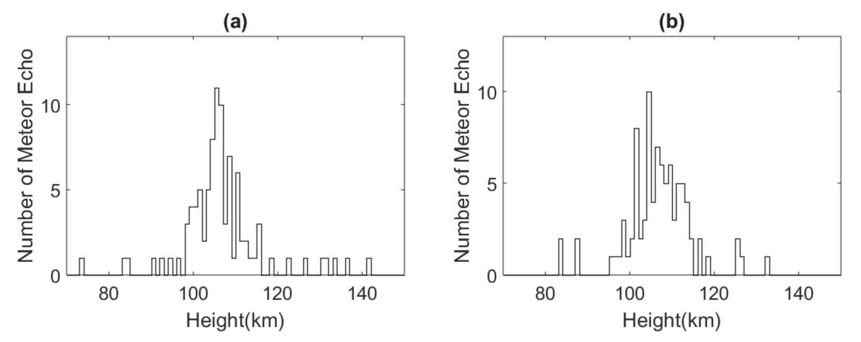
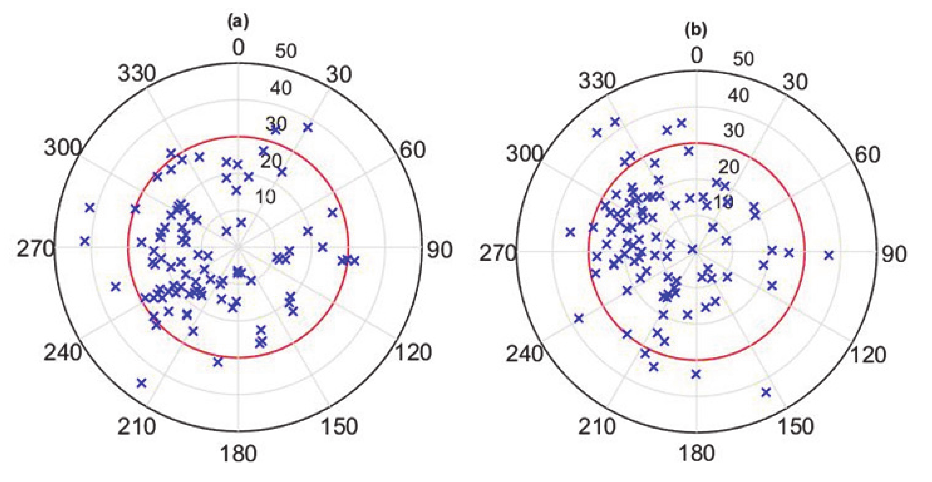
5. Meteor Distribution

We conducted nighttime meteor observations using Langfang MF radar during the Leonid meteor shower on 16 November 2017 and 17 November 2018. The observation period was 12:00–22:00 (UT). After echo detection and data analysis, we obtained 94 and 92 meteor echoes, respectively, along with their hourly echo rate, height and angular distribution.

Figure 5 shows the hourly echo rate of meteor echoes. On 16 November 2017, it starts rising at 15:00 (UT) and declines after reaching a peak at 18:00. There was an average of 9.2 meteor echoes per hour and echoes were concentrated in the 15:00–19:00 time span. Experiment on 17 November 2018 shows similar changing characteristics. Figure 6 shows meteor echo height distributions. Most echoes are detected from 90 km to 120 km. The minimum altitude was 73 km, whereas the maximum was 141 km (as shown in Figure 7). The average and peak heights were approximately 107 km and 105 km, respectively. Figure 8 shows the angular distribution of meteor echoes, demonstrating that meteor echoes are mostly distributed within zenith angles of 10°–30° and a mainly southwest azimuth.

Compared to Tsutsumi’s nighttime meteor observation at Buckland Park, Australia on 22 October 1997 [4], both experiments obtained similar spatial and height distribution of meteor echoes, concentrated in the southwest direction at an approximately 95–115 km altitude which is almost 10 km higher than traditional VHF meteor radar observations [8]. In addition, both experiments show fewer meteor echoes from 70 km to 95 km. This may be caused by the slower ambipolar diffusion at this altitude, resulting in longer echo duration, distorting meteor echoes and thus rejected by the detecting algorithm.

On the other hand, there are some differences between two experiments. Firstly, Tsutsumi reported that few out of 233 echoes in his observation were detected within 25° zenith angles and almost all the other echoes arrived from greater zenith angles, however our observation detected about 80 echoes within 30° zenith angles each time. By using vertical pencil-like beam and doughnut-like beams, Nakamura also detected many meteor echoes within 30° zenith angles [16]. Secondly, Tsutsumi has suggested that a sampling frequency of over 100 Hz should be used if echoes at 140 km need to be detected, however we successfully detected meteor echoes around 140 km altitude with practical sampling frequency of 10 Hz. Figure 7 shows a meteor echo detecting at 141 km altitude with zenith angle of 14.88°. Our observation results can be very encouraging since most MF radars are running with PRF no higher than 100 Hz.

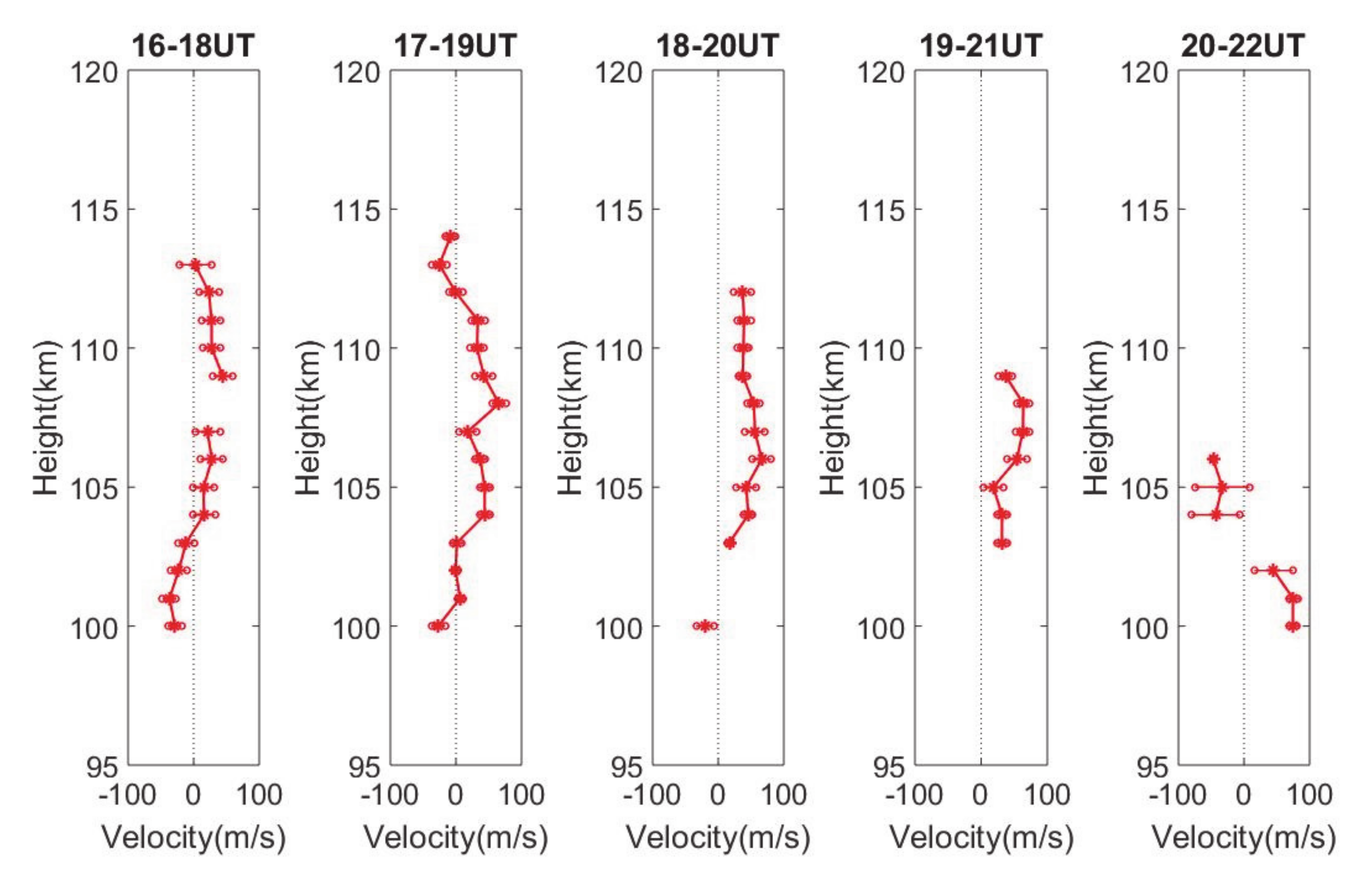
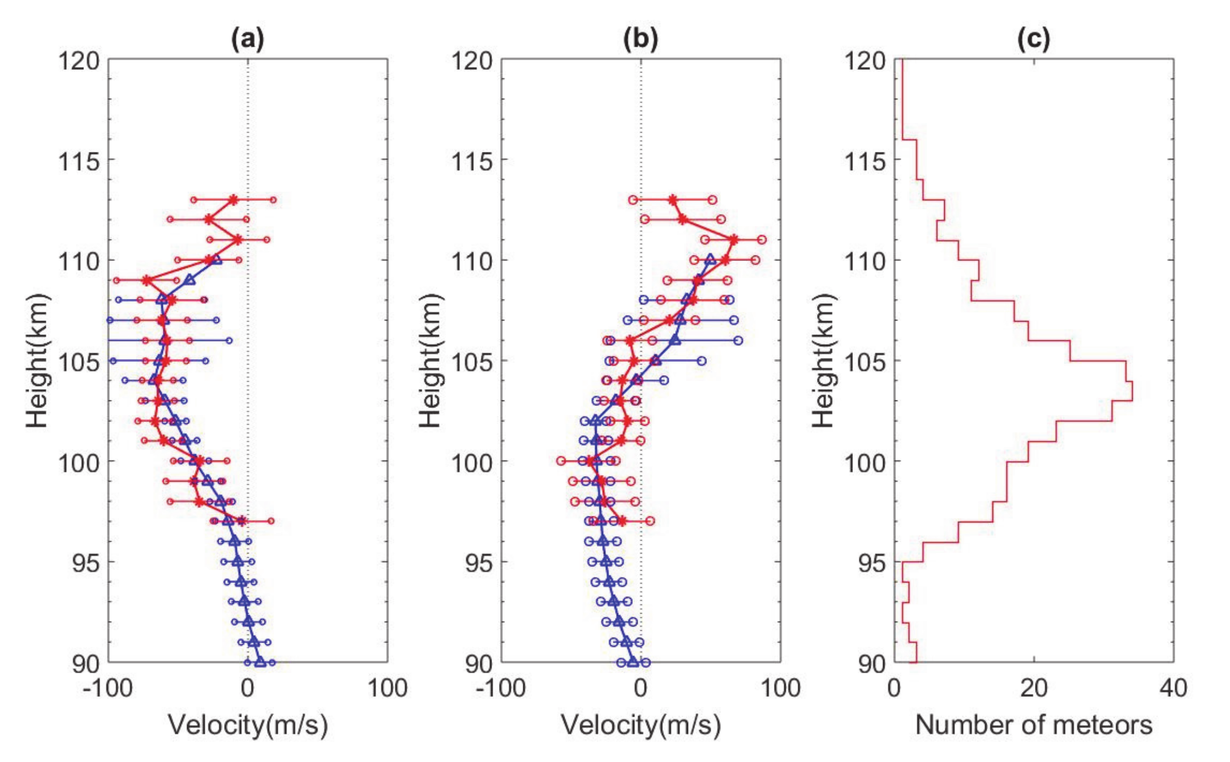
6. Horizontal Wind Estimation and Comparison

We estimated the bi-hourly and night-averaged horizontal wind velocity using meteor echoes from MF radar both on 16 November 2017 and 17 November 2018. Wind velocities were able to be estimated from 96 km to 115 km, with the upper limit nearly 10 km higher than traditional meteor radar observations. Comparisons with co-located meteor radar on 16 November 2017 were also conducted to verify the validity of the results.

Firstly, horizontal wind velocity was estimated in each time-height bin with dimensions of 2 hours and 4 km. The bin was shifted by 1 hour or 1 km, and the calculation was repeated. Bi-hourly horizontal wind profiles during 16:00–22:00 UT on 16 November 2017 and 17 November 2018 are shown in Figure 9, Figure 10, Figure 11 and Figure 12. The estimation errors were calculated in each plot (the calculation method can be referred to in Appendix A), and missing at some altitudes where wind estimation was given with only two meteor echoes. Relatively few meteor echoes were detected below 100 km and above 120 km in 2-hour time bin, and horizontal wind velocities were only given from 100 km to 120 km. On 16 November 2017, zonal wind is mostly easterly and wind shear occurs at 107 km during 20:00–22:00 UT. Meanwhile, wind shear for the meridional wind occurs at 106 km during 17:00–19:00 UT, with northerly winds becoming southerly. Additionally, zonal wind velocity is greater than meridional wind velocity. These characteristics are similar to that on 17 November 2018 except that meridional wind is mostly southerly and shows stronger fluctuation.

Secondly, averaged zonal and meridional winds from 12:00 to 22:00 UT were calculated with 4 km height bin and 1 km bin shifting. The estimation results are shown in Figure 13 and Figure 14. Since an enlarged time bin contributes to dramatic increasing in meteor echo number, averaged horizontal winds from 96 km to 115 km were successfully obtained. On 16 November 2017 zonal wind is always easterly and velocity reduces when altitude is above 109 km, whereas the meridional component is steered at 106 km, changing from northerly to southerly. On 17 November 2018 zonal wind changes from easterly to westerly at 106 km, and meridional wind is mostly southerly at altitudes below 114 km. In addition, both the zonal and meridional velocities are increasing above 100 km since thermosphere absorbs upward energy and momentum from gravity waves and tides, and downward energy from solar radiation at the same time, which enhance the air motion [17].

Horizontal wind estimation from 70 km to 110 km was also obtained by co-located VHF all-sky meteor radar on 16 November 2017. Bi-hourly and 10-hour averaged horizontal wind profiles are shown in Figure 9, Figure 10 and Figure 13. In general, VHF meteor radars have difficulty detecting a wind field above 100 km. However, during the Leonid meteor shower, we found a much higher meteor echo rate than usual, and the upper horizontal wind measurement reached 110 km.

Horizontal wind comparison results show that from 100 km to 107 km, the bi-hourly zonal winds obtained by two radars are consistent in terms of variation tendency and wind direction, and their confidence intervals are also overlapped well. Meanwhile, disagreements on some altitudes are evident in bi-hourly meridional wind profiles, although no wind reversal between them is found. In the comparison of whole night averaged zonal and meridional wind profiles shown in Figure 13, a consistent wind trend from 97 km to 110 km verifies our MF radar meteor wind estimation. Additionally, the upper height limit of the MF radar horizontal wind measurement was approximately 115 km, which is almost 10 km higher than VHF meteor radars.

Reasons for the wind velocity differences in two radars are as follows. In principle, the horizontal wind vector is fitted by employing a least squares method when more than two meteor echoes are found in each time-height bin. Fewer meteor echoes will increase uncertainty and would even lead to erroneous estimates. Therefore, meteor wind calculating under a condition of more than eight meteor echoes is more accurate and statistically significant [26]. As shown in Figure 13c, the meteor echo rate (in each time-height bin) detected by the MF radar from 97 km to 110 km is relatively high (no less than 9), which accounts for good agreement between the horizontal winds obtained by two radars at this attitude. On the other hand, the confidence of wind estimation by MF radar is not as good as that of VHF meteor radar below 100 km.

7. Conclusions

We conducted meteor observations during the Leonid meteor shower on 16 November 2017 and 17 November 2018 with Langfang MF radar. This was the first nighttime meteor observation by MF radar in mid-latitude China. By using vertical beams, 94 and 92 meteor echoes were obtained, respectively, concentrated within zenith angles of 10°–30°, from the southwest direction, and with a mean height of 107km and maximum height of 141km. Bi-hourly and night averaged horizontal wind profiles were successfully derived at the same time. Consistent horizontal wind comparison with co-located VHF meteor radar at 100–110 km altitude verifies our MF radar meteor wind estimation. The MF radar’s upper horizontal meteor wind measurement is approximately 115 km, almost 10 km higher than that of VHF meteor radar.

Though operating at different frequencies and echo peaking at different altitudes, Langfang MF radar and MU radar both obtained quite a few meteor echoes within 30° zenith angles. However, Tsutsumi has observed many more meteor echoes at greater zenith angles, as the meteor echo count is more abundant at zenith angles of 30°–50° according to MU radar’s study [16]. Relatively broad vertical beam of Langfang MF radar did not help detecting meteor echoes at zenith angles greater than 30° by using sidelobes as expected. Combining vertical and oblique antenna beams may be the optimal observation scheme if we wish to obtain the complete spatial distribution of meteor echoes. On the other hand, our observation results may suggest that meteor echoes around 140 km altitude could be detected with sampling pulse frequency less than 100Hz, proper observation scheme and signal processing, which suits for most running MF radars.

This paper gave the initial horizontal meteor wind estimation, and the nightly averaged zonal and meridional winds fit the wind estimations by the co-located VHF meteor radar. Based on these results, more wind motions and dynamic processes in the lower thermosphere, such as planetary waves, long-term prevailing wind trends, can be studied with continuous meteor wind observations. Before that, optimized antenna beam schemes are needed by using like, beam swinging in vertical and oblique directions, to increase the meteor echo count, which is the key to the statistical stability and continuous height profiling in wind estimation.

References

1. Reid, I.M.; Vandepeer, B.G.W.; Dillon, S.C. The new Adelaide medium frequency Doppler radar. Radio Sci. 1995, 30. [Google Scholar] [CrossRef]
2. Baumgaertner, A.J.G.; McDonald, A.J.; Fraser, G.J.; Plank, G.E. Long-term observations of mean winds and tides in the upper mesosphere and lower thermosphere above Scott Base, Antarctica. J. Atmos. Sol. Terr. Phys. 2005, 67, 1480–1496. [Google Scholar] [CrossRef]
3. Holdsworth, D.A.; Vandepeer, B.; Reid, I.M.; Vincent, R.A. Differential absorption measurements of mesospheric and lower thermospheric electron densities using the Buckland Park MF radar. J. Atmos. Sol. Terr. Phys. 2002, 64, 2029–2042. [Google Scholar] [CrossRef]
4. Tsutsumi, M.; Holdsworth, D.; Nakamura, T.; Reid, I. Meteor observations with an MF radar. Earth Planets Space 1999, 51, 691–699. [Google Scholar] [CrossRef] [Green Version]
5. Holdsworth, D.A. Influence of instrumental effects upon the full correlation analysis. Radio Sci. 1999, 34, 643–655. [Google Scholar] [CrossRef]
6. Cervera, M. Meteor Observations with a Narrow Beam VHF Radar; University of Adelaide: Adelaide, Australia, 1996. [Google Scholar]
7. Fahrutdinova, A.N.; Ganin, V.A.; Berdunov, N.V.; Ishmuratov, R.A.; Hutorova, O.G. Long-term variations of circulation in the mid-latitude upper mesosphere-lower thermosphere. Adv. Space Res. 1997, 20, 1161–1164. [Google Scholar] [CrossRef]
8. Olsson-Steel, D.; Elford, W.G. The height distribution of radio meteors observations at 2 MHz. J. Atmos. Sol. Terr. Phys. 1987, 49, 243–258. [Google Scholar] [CrossRef]
9. Meek, C.E.; Manson, A.H. MF radar interferometer measurements of meteor trail motions. Radio Sci. 1990, 25, 649–655. [Google Scholar] [CrossRef]
10. Tsutsumi, M.; Aso, T. MF radar observations of meteors and meteor-derived winds at Syowa (69°S, 39°E), Antarctica: A comparison with simultaneous spaced antenna winds. J. Geophys. Res. Atmos. 2005, 110, D24111. [Google Scholar] [CrossRef] [Green Version]
11. Stephen, I.G. Medium Frequency Radar Studies of Meteors; University of Adelaide: Adelaide, Australia, 2003. [Google Scholar]
12. Ceplecha, Z.; Borovička, J.; Elford, W.G.; Revelle, D.O.; Hawkes, R.L.; Porubčan, V.; Šimek, M. Meteor phenomena and bodies. Space Sci. Rev. 1998, 84, 327–471. [Google Scholar] [CrossRef]
13. Rogers, L.A.; Hill, K.A.; Hawkes, R.L. Mass loss due to sputtering and thermal processes in meteoroid ablation. Planet. Space Sci. 2005, 53, 1341–1354. [Google Scholar] [CrossRef] [Green Version]
14. Mckinley, D.W.R. Meteor Science and Engineering; McGraw-Hill Book Company, Inc.: New York, NY, USA, 1961. [Google Scholar]
15. Herlofson, N. The theory of meteor ionization. Rep. Prog. Phys. 1947, 11, 444–454. [Google Scholar]
16. Nakamura, T.; Tsutsumi, M.; Uehara, T.; Fukao, S.; Kato, S. Meteor wind observations with the MU radar. Radio Sci. 1991, 26, 857–869. [Google Scholar] [CrossRef]
17. Cervera, M.A.; Reid, I.M. Comparison of simultaneous wind measurements using colocated VHF meteor radar and MF spaced antenna radar systems. Radio Sci. 1995, 30, 1245–1261. [Google Scholar] [CrossRef]
18. Thorsen, D.; Franke, S.J.; Kudeki, E. A new approach to MF radar interferometry for estimating mean winds and momentum flux. Radio Sci. 1997, 32, 707–726. [Google Scholar] [CrossRef]
19. Cunying, X.; Xiong, H.; Qingchen, X.; Xuxing, C.; Mingliang, Z. First MF radar observations of winds and tides in the mesosphere and lower thermosphere over Langfang, China. In Proceedings of the Chinese Geophysical Society, Changsha, China, 17 November 2011. [Google Scholar]
20. Guanglin, M.; Xiong, H.; Qingchen, X.; Cunying, X. Investigation and application of FCA method for Langfang MF radar wind retrievals. Chin. J. Space Sci. 2011, 31, 618–626. [Google Scholar]
21. Meek, C.E. Triangle size effect in spaced antenna wind measurements. Radio Sci. 1990, 25, 641–648. [Google Scholar] [CrossRef]
22. Junfeng, Y.; Cunying, X.; Xiong, H.; Qingchen, X. Observations and sumulations of the mean winds in mesosphere and lower thermosphere over Langfang of China. Chin. J. Space Sci. 2017, 37, 284–290. [Google Scholar]
23. Junfeng, Y.; Cunying, X.; Xiong, H.; Qingchen, X. Seasonal variations of wind tides in mesosphere and lower thermosphere over Langfang, China (39.4°N, 116.7°E). Prog. Geophys. 2017, 32, 1501–1509. [Google Scholar]
24. Holdsworth, D.A. Signal Analysis with Applications to Atmospheric Radars; University of Adelaide: Adelaide, Australia, 1995. [Google Scholar]
25. Hocking, W.K.; Fuller, B.; Vandepeer, B. Real-time determination of meteor-related parameters utilizing modern digital technology. J. Atmos. Sol. Terr. Phys. 2001, 63, 155–169. [Google Scholar] [CrossRef]
26. Holdsworth, D.A.; Reid, I.M.; Cervera, M.A. Buckland Park all-sky interferometric meteor radar. Radio Sci. 2004, 39, RS5009. [Google Scholar] [CrossRef]
27. Vandepeer, B.W.; Reid, I.M. Some preliminary results obtained with the new Adelaide MF Doppler radar. Radio Sci. 1995, 30, 1191–1203. [Google Scholar] [CrossRef]
28. Vandepeer, B. A New MF Doppler Radar for Upper Atmospheric Research; University of Adelaide: Adelaide, Australia, 1993. [Google Scholar]
29. Sato, T. Radar Principles. Handb. MAP 1989, 30, 19–53. [Google Scholar]
Figure 1. Langfang medium frequency (MF) radar antenna array.
Atmosphere 11 00507 g001
Figure 2. Langfang MF radar raw data: (a) before filtering; (b) after filtering; the color coded in the figures stands for radar signal strength.
Atmosphere 11 00507 g002
Figure 3. Amplitude and phase of a typical meteor echo. The red dashed line refers to the amplitude threshold of meteor detection.
Atmosphere 11 00507 g003
Figure 4. Phase offset between receiver 3 and receiver 4. The mean value is 2.94 degrees according to the red dashed line.
Atmosphere 11 00507 g004
Figure 5. Hourly echo rate of meteor echoes: (a) 16 November 2017, (b) 17 November 2018.
Atmosphere 11 00507 g005
Figure 6. Height distribution of meteor echoes: (a) 16 November 2017, (b) 17 November 2018.
Atmosphere 11 00507 g006
Figure 7. Meteor echoes at 73km (left) and 141km (right).
Atmosphere 11 00507 g007
Figure 8. Angular distribution of meteor echoes: (a) 16 November 2017, (b) 17 November 2018.
Atmosphere 11 00507 g008
Figure 9. Bi-hourly zonal wind profiles on 16 November 2017: red lines refer to MF radar results and blue lines refer to meteor radar results.
Atmosphere 11 00507 g009
Figure 10. Bi-hourly meridional wind profiles on 16 November 2017: red lines refer to MF radar results and blue lines refer to meteor radar results.
Atmosphere 11 00507 g010
Figure 11. Bi-hourly zonal wind profiles on 17 November 2018.
Atmosphere 11 00507 g011
Figure 12. Bi-hourly meridional wind profiles on 17 November 2018.
Atmosphere 11 00507 g012
Figure 13. Averaged horizontal wind on 16 November 2017: red lines refer to MF radar results and blue lines refer to meteor radar results: (a) zonal wind; (b) meridional wind; (c) number of meteors.
Atmosphere 11 00507 g013
Figure 14. Averaged horizontal wind on 17 November 2018: (a) zonal wind; (b) meridional wind; (c) number of meteors.
Atmosphere 11 00507 g014