Retrieval of Cloud Liquid Water Using Microwave Signals from LEO Satellites: A Feasibility Study through Simulations

Abstract

A novel approach, using low Earth orbit (LEO) satellite microwave communication links for cloud liquid water measurements, is proposed in this paper. The feasibility of this approach is studied through simulations of the retrieval system including a LEO satellite communicating with a group of ground receivers equipped with signal-to-noise ratio (SNR) estimators, a synthetic cloud attenuation field and a tomographic retrieval algorithm. Rectangular and Gaussian basis functions are considered to define the targeted field. Simulation results suggest that the proposed least-squares based retrieval algorithm produces satisfactory outcomes for both types of basis functions. The root-mean-square error of the retrieved field is around 0.2 dB/km, with the range of the reference field as 0 to 2.35 dB/km. It is also confirmed that the partial retrieval of the cloud field is achievable when a limited number of receivers with restricted locations are available. The retrieval outcomes exhibit properties of high resolution and low error, indicating that the proposed approach has great potential for cloud observations.

1. Introduction

Understanding the role of clouds is of great importance in many areas such as numerical weather prediction and climate studies, as clouds are not only vital in the hydrological cycle, but also crucial for the Earth’s radiation budget. Various instruments have been developed and deployed, such as microwave radiometers, cloud radars and lidars, to measure cloud liquid water content (LWC) on a fine scale [1]. However, due to the high cost and scarce distribution of such instruments, the real-time global seamless high-resolution observation of clouds is still a challenge.

In this paper, we propose a novel cloud estimation approach as an auxiliary means to traditional methods, in which the attenuation of low Earth orbit (LEO) satellite microwave links is used to measure the LWC in clouds. Currently, the number of active LEO satellites in space is well above 1000, and several companies are pursuing the proposal for large constellations of LEO satellites to provide global broadband access, e.g., OneWeb’s system with 720 LEO satellites for global coverage and SpaceX’s system with more than 4000 LEO satellites [2]. Once this service is available to the public, it can be foreseen that millions of user terminals (ground receivers) will be deployed across the globe. Because of the high demand for bandwidth, Ku-band (12~18 GHz) and Ka-band (26.5~40 GHz) are usually used for downlink and uplink. These links are sensitive to the water content in the atmosphere. Essentially, the communication links between the satellites and the user terminals maintain a very large sensor network that could provide off-the-shelf attenuation data for the purpose of atmospheric observations.

The hypothesis of using LEO satellite microwave links for atmospheric measurements was first proposed in 2016 [3], where moving microwave links were used to achieve rain field estimations. Similar to the motion of the signal source in computed tomography (CT) [4], the orbital motions of the LEO satellites make it possible to perform tomographic reconstruction of rain fields. Various investigations have been carried out recently. For example, it has been shown that vertical rain fields can be reconstructed from the received signal level measurements of multiple receivers [5]. Furthermore, the approach of using the estimated signal-to-noise ratio (SNR) at the ground receivers for LEO satellites to achieve three-dimensional (3-D) tomographic rain field reconstruction has been analyzed in detail [6].

The focus of this paper is on using LEO satellite-to-ground signal links for cloud measurements. The same system model used for rain field retrieval [6] is employed for retrieving the attenuation field caused by nonprecipitating clouds. Although the attenuation induced by clouds is usually considerably less than that induced by rain, it is still significant enough in signal power measurements. For instance, for a LWC of 1 g/m³, the specific attenuation at 30 GHz is about 0.88 dB/km [7]. This indicates that accurate LWC measurements can be achieved through accurately measured signal attenuations. The first objective of this study is to confirm that the SNR estimations at the ground receivers, subject to noise and estimation errors, can be used to retrieve cloud LWC induced attenuation fields through tomographic techniques. The second objective is to extend and refine previous studies on rain field retrieval [6], by introducing different basis functions to define the target attenuation field. Moreover, to cope with the sky noise induced by rain or cloud LWC, a reduced-complexity method of post-processing with a piecewise linear function is proposed and compared with the existing iterative approach [6].

This study only addresses cloud liquid water, and solid particles such as ice crystals and snow are not considered as they have minimal effects on the attenuation of microwave signals around 30 GHz [8]. Compared with rain field retrieval, besides the size difference between rainwater drops and cloud water drops, another major difference is the altitude of the drops in the atmosphere. Raindrops usually exist from the ground up, while the cloud bottom is mostly at least several hundred meters above ground [9]. Consequently, the blind zone near the ground, due to receivers’ minimum elevation angle requirement [6], will have less impact on the cloud LWC retrieval than on rainwater.

To test the feasibility of the cloud LWC measurement proposal, we utilize a synthetic cloud field generated by the Weather Research and Forecasting (WRF) model [10,11] version 3.9.1.1. The cloud field is from an idealized simulation of a mesoscale convective system (MCS) initialized with a central U.S. MCS inflow sounding [12]. It is expected to include realistic cloud microphysics and cloud dynamics [13]. The model horizontal and vertical grid spacing is 250 m. Combining a LEO satellite trajectory with a satellite-to-ground signal model, we simulate the SNR estimation at the ground receivers and then use a tomographic algorithm to retrieve the attenuation field induced by the cloud LWC. It is assumed that only the SNR estimation is available at the receivers and that parameters including the transmitted signal power, the system noise power, and the attenuation due to other factors are unknown. The sky noise generated by cloud radiation is modelled and simulated, too. Because of the nonlinear relation between the sky noise and the path-integrated attenuation, a piecewise linear function is proposed to post-process the retrieved attenuation field in order to counterbalance the attenuation effects of the sky noise. Different basis functions for the attenuation field are introduced and simulated, with their effects on cloud field retrieval analyzed. Simulation results show that the proposed approach has great potential for cloud attenuation field retrieval. Even with a limited number of receivers with restricted locations, the partially retrieved field is still satisfactory.

The rest of this paper is organized as follows. A detailed description of the system model can be found in Section 2. The proposed attenuation field retrieval method is presented in Section 3. Numerical results in regard to the synthetic cloud field and the tomographic retrieval under different conditions are given in Section 4. Finally, Section 5 concludes this paper.

2. System Model

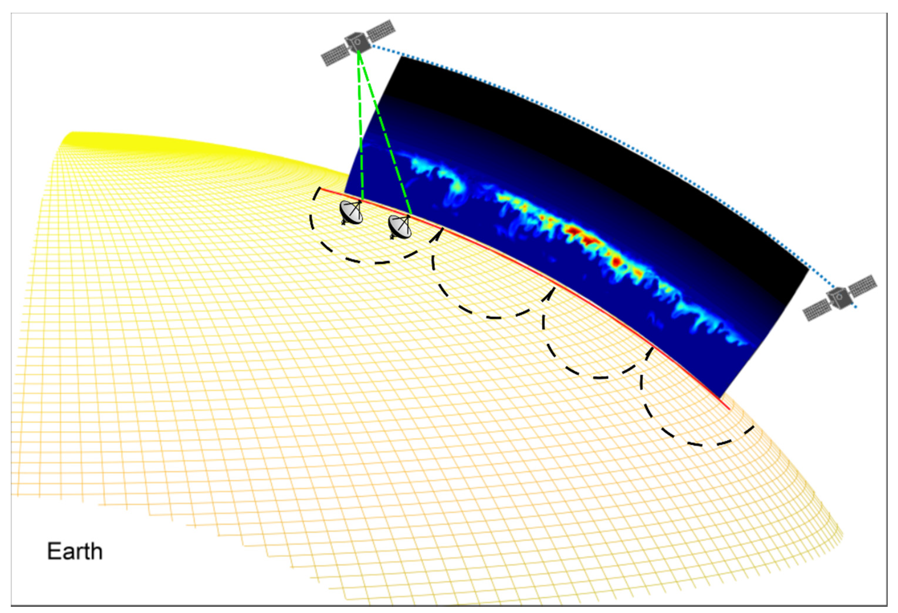
2.1. Orbital Geometry

This model consists of a LEO satellite that passes over a cloud and multiple ground receivers equipped with electronically steerable phased array antennas [14]. The overpass time is determined by the orbital parameters of the satellite and the minimum elevation angle of the ground receivers. The satellite has a direct spot beam to the ground receivers, and the receivers use their antennas’ steering capability to track the transit of the satellite. The SNRs at the ground receivers are estimated for the purpose of measuring the path-integrated attenuation.

During a single overpass, the signal link between a satellite and a ground receiver moves along a curved surface, thereby the attenuation caused by water droplets on this surface can be detected by the SNR estimation at the receiver. If we consider the scenario where the satellite passes directly over the receiver, the curved surface can be regarded as flat because the curvature is purely induced by the slight Earth rotation during the overpass and can be ignored. When multiple receivers are placed along the ground track of the satellite, the moving signal links will cover most of the vertical plane [6], and thereby offer the possibility of retrieving the vertical attenuation field. An illustration of the orbital geometry and the targeted attenuation field is shown in Figure 1. Depending on the satellite system, the surface coverage of a single beam could vary from 2800 km² to 72,000 km² [2]. An example of the −3 dB footprint contour is shown by the black dashed lines in Figure 1. Each satellite can achieve a data-rate above 20 Gbps [2], which means that it can easily serve 10,000 user terminals (assuming 2 Mbps bandwidth each) simultaneously within a beam.

The proposed method can be easily extended to 3D attenuation field retrieval with additional receivers placed in a two-dimensional array on the ground. Previous studies have shown that 3D tomographic attenuation field reconstruction can be achieved through the aggregation of a series of reconstructed vertical planes [6]. This paper will only focus on the retrieval of one vertical cloud attenuation field.

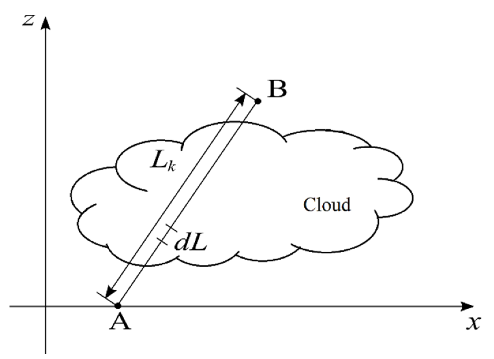
2.2. Signal Attenuation Model

The signal attenuation model used here is the same as those in previous studies [6,15]. The signal power at a ground receiver is obtained by

$$P_r={\xi }_I\times {\xi }_F\times {\xi }_C\times P_t+P_n,$$

(1)

in which the power of the received signal and the power of the transmitted signal at the satellite are denoted by $P_r$ and $P_t$, respectively. The power of noise is denoted by $P_n$, which includes both the system noise and the sky noise. The channel gain in Equation (1) is determined by three major factors: ${\xi }_I$ is the path-integrated cloud attenuation, ${\xi }_F$ is the free space power loss (FSPL) and ${\xi }_C$ represents the attenuation due to all other factors such as the gain of antennas and effects of water vapor. Suppose that there are $M$ signal samples available at the receiver over the duration the overpass of the satellite. Each sample is acquired from a different and very short (0.05 s in the simulations) time window. For the $k$-th sample, the receiver’s SNR in decibels is obtained by

$$\rho \left(k\right)=10·\log \frac{{\xi }_I\left(k\right)\times {\xi }_F\left(k\right)\times {\xi }_C\left(k\right)\times P_t\left(k\right)}{P_n\left(k\right)}, k=1,2,\cdots , M.$$

(2)

We define $A_I\left(k\right)$ as the path-integrated cloud attenuation in decibels as

$$A_I\left(k\right)=-10\times \log \left({\xi }_I\left(k\right)\right),$$

(3)

and the free space loss $A_F\left(k\right)$ is obtained by

$$A_F\left(k\right)=-10\times \log \left({\xi }_F\left(k\right)\right),$$

(4)

thus, $\rho \left(k\right)$ can be rewritten as

$$\rho \left(k\right)=10\times \log \frac{{\xi }_C\left(k\right)\times P_t\left(k\right)}{P_n\left(k\right)}-A_I\left(k\right)-A_F\left(k\right).$$

(5)

Let the noise temperature of the receiving system and the sky temperature be denoted by $T_{sys}\left(k\right)$ and $T_{sky}\left(k\right)$, in Kelvin, respectively. In this case, noise power $P_n\left(k\right)$ is obtained by [16]

$$P_n\left(k\right)=k_B\times B\times \left(T_{sys}\left(k\right)+T_{sky}\left(k\right)\right),$$

(6)

where $k_B$ is the Boltzmann constant and $B$ is the bandwidth of the communication system. We define parameter $C\left(k\right)$ as

$$C\left(k\right)=10\times \log \frac{{\xi }_C\left(k\right)\times \left(k\right)}{k_B\times B\times T_{sys}\left(k\right)},$$

(7)

and noise figure $F_n\left(k\right)$ as

$$F_n\left(k\right)=10\times \log \left(\frac{T_{sys}\left(k\right)+T_{sky}\left(k\right)}{T_{sys}\left(k\right)}\right),$$

(8)

according to Equation (5), $\rho \left(k\right)$ is then obtained by

$$\rho \left(k\right)=C\left(k\right)-F_n\left(k\right)-A_I\left(k\right)-A_F\left(k\right).$$

(9)

Parameter $C\left(k\right)$ can be regarded as a baseline value for a receiver, which is mainly determined by the noise temperature of the receiving system, the antenna gain and the power of the transmitted signal. In this model, cloud is the primary source for $T_{sky}\left(k\right)$, which is generally obtained by [17]

$$T_{sky}\left(k\right)=\frac{{{\displaystyle \int }}^{}G\left(k,\mathsf{\Omega }\right)T\left(\mathsf{\Omega }\right)d\mathsf{\Omega }}{{{\displaystyle \int }}^{}G\left(k,\mathsf{\Omega }\right)d\mathsf{\Omega }},$$

(10)

where $\mathsf{\Omega }$ is the solid angle, $G\left(k,\mathsf{\Omega }\right)$ is the antenna gain pattern and $T\left(\mathsf{\Omega }\right)$ is the noise temperature for a particular direction determined by $\mathsf{\Omega }$, which is obtained by

$$T=t_m\left(1-{10}^{-\frac{A_I}{10}}\right),$$

(11)

where $t_m$ is the mean path temperature, in Kelvin, and $A_I$ is the total path attenuation for that direction, in dB. We assume that the beam pattern of the antenna is known so the relation between $T_{sky}$ and $A_I$ can be established using Equations (10) and (11).

Meanwhile, $A_F\left(k\right)$ is a function of the satellite-to-ground path length $L_S$ and the signal frequency $f$, and is commonly obtained by [18]

$$A_F\left(k\right)=20\times \log \left(L_S\left(k\right)\right)+20\times \log \left(f\right)+92.45,$$

(12)

where the unit of $L_S\left(k\right)$ is in km and $f$ in GHz. Since $A_F\left(k\right)$ can be regarded as known, Equation (9) indicates that $A_I\left(k\right)$ has the following relation with the SNR estimation:

$$A_I\left(k\right)=C\left(k\right)-\widehat{\rho }\left(k\right)-A_F\left(k\right)-F_n\left(k\right),$$

(13)

where $\widehat{\rho }\left(k\right)$ is the estimated SNR at the receivers.

3. Retrieval Method

With $A_F\left(k\right)$ and $\widehat{\rho }\left(k\right)$ known, the retrieval process mainly involves handling the two unknown terms $C\left(k\right)$ and $F_n\left(k\right)$ as well as solving the cloud attenuation field.

Consider a vertical rectangular attenuation field of interest. As the overpass time is very short for the LEO satellite (e.g., 289 s for a satellite at 1000 km of orbital height and a minimum elevation angle of 40 degrees for ground receivers), the attenuation field is regarded as static for the purpose of retrieval. It is described by a function of two variables $R\left(x,z\right)$ representing the specific attenuation in dB/km at coordinates $\left(x,z\right)$ km, where the $x$-axis represents the horizontal direction along the ground track of the satellite and the $z$-axis is the vertical direction starting from sea level. The relation between the path-integrated attenuation and the attenuation field function is obtained by [19]

$$A_I\left(k\right)={{\displaystyle \int }}_{L_k}R\left(x,z\right)dL,$$

(14)

where $L_k$ denotes the signal line path for the $k$-th sample (see Figure 2).

It is assumed that $R\left(x,z\right)$ can be approximated by a linear combination of $N$ basis functions ${\left\{b_n\left(x,z\right)\right\}}_{n=1}^N$:

$$R\left(x,z\right)={{\displaystyle \sum }}_{n=1}^N{w}_n{b}_n\left(x,z\right),$$

(15)

where $w_n$ is the weight for $b_n$. Equation (14) then becomes

$$A_I\left(k\right)={{\displaystyle \sum }}_{n=1}^N{w}_n{{\displaystyle \int }}_{L_k}{b}_n\left(x,z\right)dL.$$

(16)

We define

$$q_{k,n}={{\displaystyle \int }}_{L_k}{b}_n\left(x,z\right)dL,$$

(17)

and $q_{k,n}$ represents the line integral of the $n$-th basis function along the $k$-th sample path. Once the basis functions have been determined, $q_{k,n}$ can be obtained solely from the geometrical conditions of the satellite and the ground receiver at the time that the signal is sampled. As a result, $q_{k,n}$ can be calculated offline and stored away for later use.

If the path-integrated attenuation $A_I$ can be measured, the retrieval task then becomes a matter of solving the series weights ${\left\{w_n\right\}}_{n=1}^N$. However, the path-integrated attenuation is only measured indirectly through the SNR estimation. We rewrite Equation (13) as

$$C\left(k\right)-V\left(k\right)-F_n\left(k\right)={{\displaystyle \sum }}_{n=1}^N{w}_n{q}_{k,n},$$

(18)

where $V\left(k\right)$ is the sum of two known terms:

$$V\left(k\right)=\widehat{\rho }\left(k\right)+A_F\left(k\right).$$

(19)

Note that $A_F\left(k\right)$ can be calculated by Equation (12) but $C\left(k\right)$ and $F_n\left(k\right)$ are unknown. For a similar problem in [6], $C\left(k\right)$ is regarded as a constant and solved together with ${\left\{w_n\right\}}_{n=1}^N$ using a least-squares method. However, in reality, parameter $C\left(k\right)$ could change during one overpass [15,20], so forcing it to be a constant could introduce considerable errors. An improved approach [15] to eliminate $C\left(k\right)$ before solving ${\left\{w_n\right\}}_{n=1}^N$ was introduced as follows. Considering another sample link ($k+\mathsf{\Delta }$) which is very close in time to sample link $k$, Equation (18) becomes

$$C\left(k+\mathsf{\Delta }\right)-V\left(k+\mathsf{\Delta }\right)-F_n\left(k+\mathsf{\Delta }\right)={{\displaystyle \sum }}_{n=1}^N{w}_n{q}_{k+\mathsf{\Delta },n}.$$

(20)

The difference between $C\left(k+\mathsf{\Delta }\right)$ and $C\left(k\right)$ is ignored because the two links are very close in time, Equations (18) and (20) yield

$$V\left(k\right)-V\left(k+\mathsf{\Delta }\right)+F_n\left(k\right)-F_n\left(k+\mathsf{\Delta }\right)={{\displaystyle \sum }}_{n=1}^N{w}_n(q_{k+\mathsf{\Delta },n}-q_{k,n}),$$

(21)

Without prior knowledge of the path-integrated attenuation, noise figure $F_n\left(k\right)$ is completely unknown. One viable approach is to initially regard $F_n\left(k\right)$ as zero for the first least-squares computing. According to Equation (8), this means that $T_{sky}$ is zero, which is physically incorrect [21]. However, it has been shown that the retrieved ${\left\{w_n\right\}}_{n=1}^N$ can be used to update $F_n\left(k\right)$ and in turn correct ${\left\{w_n\right\}}_{n=1}^N$ in an iterative manner [6]. In this paper, we adopt this iterative approach, as well as explore an alternative way of processing the first retrieval result directly to achieve satisfactory estimations, which is discussed in detail in Section 4.

For the first iteration, we regard $F_n\left(k\right)$ as zero and consider Equation (21) in the matrix form

$$Y=\overline{Q}·w,$$

(22)

where $w$ is ${\left\{w_n\right\}}_{n=1}^N$ and $\overline{Q}$ is the $\left(M-\mathsf{\Delta }\right)\times N$ differential matrix:

$$\overline{Q}= \left[\begin{array}{cccc}{q}_{1+\mathsf{\Delta },1}-q_{1,1}& q_{1+\mathsf{\Delta },2}-q_{1,2}& \cdots & q_{1+\mathsf{\Delta },N}-q_{1,N}\\ q_{2+\mathsf{\Delta },1}-q_{2,1}& q_{2+\mathsf{\Delta },2}-q_{2,2}& \cdots & q_{2+\mathsf{\Delta },N}-q_{2,N}\\ ⋮& ⋮& ⋮& ⋮\\ q_{M,1}-q_{M-\mathsf{\Delta },1}& q_{M,2}-q_{M-\mathsf{\Delta },2}& \cdots & q_{M,N}-q_{M-\mathsf{\Delta },N}\end{array}\right]$$

(23)

and for $Y$

$$Y\left(k\right)=V\left(k\right)-V\left(k+\mathsf{\Delta }\right), k=1,2,\cdots , M-\mathsf{\Delta }.$$

(24)

We then solve Equation (22) by formulating the following linear least-squares problem

$$\widehat{w}=\arg \min S\left(w\right), \mathrm{subject} \mathrm{to} w_n\ge 0, 1\le n\le N,$$

(25)

where

$$S(w)={\Vert Y-\overline{Q}·w\Vert }^2.$$

(26)

From the second iteration, $F_n\left(k\right)$ is updated using Equations (8) and (10), $Y\left(k\right)$ is updated by $Y\left(k\right)=V\left(k\right)-V\left(k+\mathsf{\Delta }\right)+F_n\left(k\right)-F_n\left(k+\mathsf{\Delta }\right)$, and the least-squares problem (25) is run again to update ${\left\{w_n\right\}}_{n=1}^N$.

Two types of basis functions are investigated in this paper. The first is a two-dimensional rectangular function obtained by

$${\tau }_n\left(x,z\right)=\{\begin{array}{ll}1 \left(\mathrm{dB}/\mathrm{km}\right),& \mathrm{for} \left|x-X_n\right|<\frac{u}{2} \mathrm{and} \left| z-Z_n\right|<\frac{u}{2}\\ 0 \left(\mathrm{dB}/\mathrm{km}\right),& \mathrm{otherwise}\end{array},$$

(27)

where $u$ is the width of the rectangular function and $(X_n, Z_n)$ is the center coordinate of the $n$-th function. Essentially, the rectangular basis functions offer a way to cover the field of interest with a regular grid. The integral $q_{k,n}$ is simplified to the length of the $k$-th link within the $n$-th unit square.

The second type of basis function is a Gaussian basis function defined by [22]

$${\mu }_n\left(x,z\right)=\exp \left(-\frac{{\delta }_{x,z,n}^2}{2{\sigma }^2}\right) \left(\mathrm{dB}/\mathrm{km}\right),$$

(28)

where ${\delta }_{x,z,n}$ is the distance from $\left(x,z\right)$ to the center of the $n$-th basis function located at $(X_n, Z_n)$

$${\delta }_{x,z,n}=\sqrt{{\left(x-X_n\right)}^2+{\left(z-Z_n\right)}^2},$$

(29)

and $\sigma$ is the width of the Gaussian functions.

Note that no matter which basis function is applied, the differential matrix $\overline{Q}$ can be calculated offline before using the least-squares.

4. Simulation Results

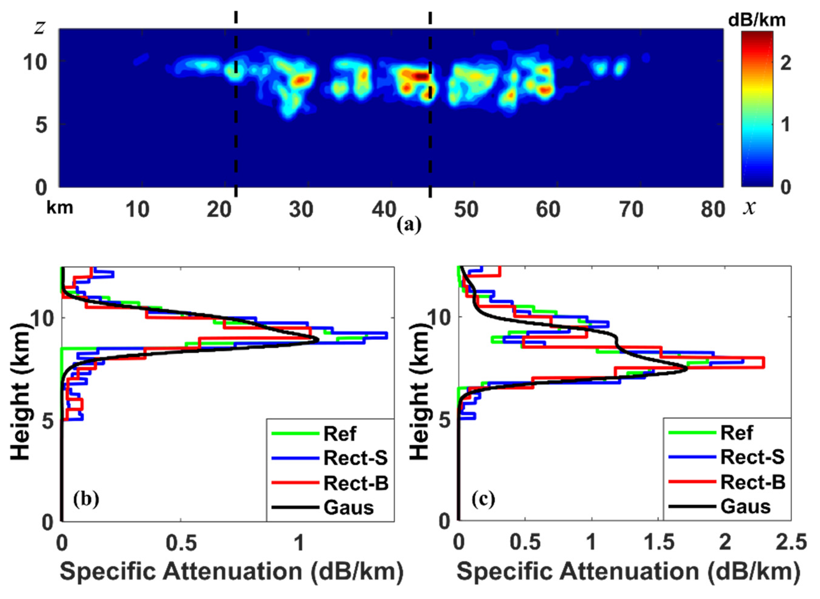
4.1. Synthetic Attenuation Field

The synthetic cloud data used in this paper were produced from an idealized simulation of a mesoscale convective system using the WRF model. More details about the simulation can be found in Ref. [12]. This cumulus type cloud has very large vertical development, the cloud base is approximately 5 km in height, with the top around 10 km. One vertical slice of the cloud field that covers 80 km in width and 0–12.5 km in height was selected as the reference field. This slice contains a very high content of water, which mainly consists of supercooled cloud water. Some areas can produce specific attenuation up to 2.35 dB/km, while there are other areas with relatively thin clouds. Very few rainwater droplets are present in this slice. A 320 × 50 grid is used to define the field with each unit square being 250 m by 250 m, i.e., both the horizontal and vertical resolutions are 250 m.

In the cloud LWC field generated by WRF, each unit square has a uniform cloud water mixing ratio given in g/g, which is defined as

$$\beta ={\omega }_w/{\omega }_a,$$

(30)

where ${\omega }_w$ and ${\omega }_a$ are the liquid water and dry air density in g/m³, respectively. Note that other particles such as ice crystals and snow are not considered as they have minimal effects on the attenuation of microwave signals around 30 GHz [8].

Dry air density is obtained by [23]

$${\omega }_a=11.612p\times \frac{300}{T_c},$$

(31)

in which $T_c$ is the cloud liquid water temperature in Kelvin and $p$ is the dry air pressure in kPa. We use the barometric law [24] to calculate $p$:

$$p\left(z\right)=P_0\times {\left(\frac{T_0}{T_0+L_b\times z}\right)}^{\frac{g_0\times M_e}{R_0\times L_b}},$$

(32)

where $z$ is the altitude above sea level, $P_0$ is static pressure at sea level (101.325 kPa), $g_0$ is gravitational acceleration (9.80655 m/s²), $M_e$ is molar mass of Earth’s air (0.0289644 kg/mol) and $R_0$ is universal gas constant (8.3144598 J/(mol·K)). For each unit square in the cloud field, temperature $T_c$ is calculated according to the altitude of the center of the square, assuming that the temperature lapse rate $L_b$ is −0.0065 K/m from the sea level temperature $T_0$ of 288 K. Note that the constant lapse rate is an approximation for the cloudy atmosphere and will introduce an inaccuracy in the temperature profile. Nevertheless, it only serves as a means to translate the WRF-generated LWC field into the reference attenuation field, and using it does not affect the validation of the retrieval method per se.

In order to generate the reference attenuation field, we use the equations provided by the International Telecommunications Union (ITU) [25], where the specific attenuation within a cloud is obtained by

$$R\left(f,T_c\right)=K_l\left(f,T_c\right){\omega }_w,$$

(33)

where $K_l$ is the cloud liquid water specific attenuation coefficient (details can be found on Page 2 in [25]) in (dB/km)/(g/m³), $f$ is the signal frequency in GHz. With the temperature and pressure profile ready for each unit square, ${\omega }_w$ can be calculated using Equations (30) and (31) and the specific attenuation $R$ can then be calculated by Equation (33) with the signal frequency $f=30$ GHz. The reference attenuation field is shown in Figure 3a.

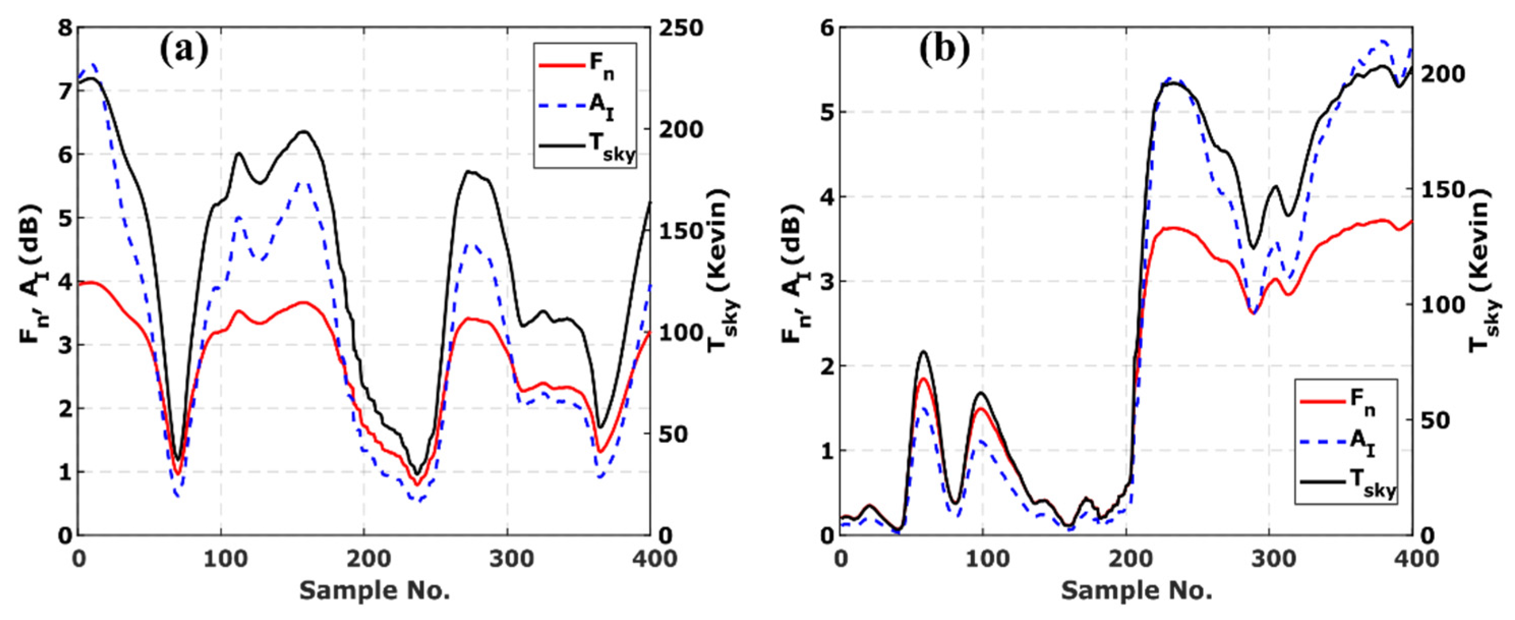
4.2. Simulation of the Estimated SNR

We considered a LEO satellite with a circular Keplerian motion trajectory of an orbital height of 1000 km and an inclination angle of 96°. The trajectory is on the same vertical plane as the cloud attenuation field of interest. There are 91 receivers evenly placed at the ground level, with any two adjacent receivers being 1 km apart. The first and the last receivers are located at $x=-5$ km and $x=85$ km in Figure 3a, respectively. With the assumption that the minimum elevation angle for the receivers is 40°, it can be calculated that the overpass time is approximately 289 s. We use 400 signal samples ($M=400$) during the satellite overpass time for each receiver. The samples are taken at fixed time intervals, i.e., the overpass time is evenly divided by the 400 samples.

The observation window for each sample is chosen as 0.05 s. According to previous results [6], the error induced by satellite movement in the observation window is significantly lower than the Cramer–Rao Lower Bound (CRLB) of the SNR estimation. Consequently, the path-integrated cloud attenuation $A_I$ and the free space loss $A_F$ are calculated only for the starting point of the observation window and assumed to remain the same within the window. The estimated SNR $\widehat{\rho }$ for each sample of each receiver is simulated in the following steps:

• For each receiver, preset the constant $C$ along a sine curve between 214 dB and 216 dB to simulate the differences across different receivers.
• Calculate the path-integrated attenuation $A_I\left(k\right)$ and the free space loss $A_F\left(k\right)$ using Equations (12) and (14), respectively.
• The sky noise temperature $T_{sky}\left(k\right)$ is computed according to the cloud attenuation from nine different directions and a simplified antenna beam pattern (Equations (10) and (11) with $t_m=275$ K, see [6] for details). Noise figure $F_n\left(k\right)$ is then calculated using Equation (8) with $T_{sys}=150$ K.
• The true SNR is then calculated using Equation (9).
• We assume a Binary Phase Shift Keying (BPSK) modulated signal with a bit rate of 10 Mbps and the estimated SNR $\widehat{\rho }$ is generated by adding the true SNR to a Gaussian random variable with zero mean and variance being equal to the CRLB.

4.3. Retrieval Using Rectangular Basis Functions

In this section, we use $N$ rectangular basis functions obtained by Equation (27) to retrieve the attenuation field. Here, $N$ is assumed to be 320 × 50 and width $u$ for each function to be 250 m. In other words, the retrieved attenuation field is defined by a grid exactly the same as that of the reference field.

Theoretically, parameter $\mathsf{\Delta }$ for the differential approach in Equation (21) needs to be small so that the assumption that $C\left(k\right)$ stays static can be met. However, simulations show that $\mathsf{\Delta }=1$ will generally make the differential distances ($q_{k+\mathsf{\Delta },n}-q_{k,n}$) very close to zero and thus make the algorithm sensitive to noise and estimation errors. After some experiments, parameter $\mathsf{\Delta }$ is set at 3, which seems to produce the best retrieval outcomes. After calculating the differential matrix $\overline{Q}$, a constrained least-squares algorithm using an interior-point method (lsqlin in Matlab, see [26,27]) is employed. The upper and lower bounds for $w_n$ are set to 5 and 0, respectively. In addition, we assume that there being no cloud in the bottom 320 × 20 unit squares is prior knowledge. In all of the following simulations, therefore, the weights for the basis functions below 5 km are considered zero and only the weights for the basis functions above 5 km (320 × 30 basis functions in this case) are retrieved. Figure 3b shows the retrieved attenuation field obtained by the least-squares algorithm. Note that the retrieved specific attenuation is greater than the reference value (overestimation) for many of the unit squares. This is because, in the first iteration of the algorithm, by assuming $F_n$ in Equation (13) to be zero, the impact of $F_n$ is included in the path-integrated attenuation $A_I$ and makes it effectively larger. The retrieved attenuation field can be used to update $F_n$ and therefore enable the second iteration of the least-squares. The second retrieved field will be underestimated because $F_n$ is overestimated, as the attenuation field is overestimated in the first iteration. As a result, the retrieved fields will oscillate between iterations, but averaging the attenuation fields of two consecutive iterations will yield satisfactory results for rain field estimation [6]. Figure 3c shows the final retrieved field by averaging the third and fourth iterations. It can be seen that, for both heavy cloud areas where there is large vertical development and thin cloud areas, the retrieved field and the reference field have good agreement.

Assuming that the ground receiver antenna has high directivity, we can simplify the relation between the sky noise and the path-integrated attenuation by assuming that the sky temperature picked up by the antenna is from one direction only, i.e.,

$$T_{sky}\left(k\right)=t_m\left(1-{10}^{-\frac{A_I\left(k\right)}{10}}\right).$$

(34)

As a result, from Equations (8) and (34), we can conclude that $F_n$ increases with $A_I$ in a nonlinear manner. The nonlinear relation can be observed in Figure 4, where $F_n$ (red line), $A_I$ (blue dashed line) and $T_{sky}$ (black line) are plotted over the entire course of the overpass. The left panel is for the receiver located at 40 km and the right panel is for the receiver located at 60 km. The ratio of $F_n/A_I$ is large for small $A_I$ (e.g., $\frac{F_n}{A_I}\approx 1.8$ when $A_I=0.1$ dB) and is small for large $A_I$ (e.g., $\frac{F_n}{A_I}\approx 0.6$ when $A_I=6$ dB).

For the iterative approach that generates Figure 3c, the least-squares computing needs to be run four times, and each time it deals with $400\times 91=\mathrm{36,400}$ equations. The relation between $A_I$ and $F_n$ in the above can be utilized to reduce the number of the least-squares computing to one time only, thereby reduce the computing complexity of the retrieval process. We propose the following piecewise linear (PL) function to process the retrieved ${\left\{{\widehat{w}}_n\right\}}_{n=1}^N$ after the first least-squares computing:

$$w_n^{\prime }=\frac{{\widehat{w}}_n}{B\left({\widehat{w}}_n\right)},$$

(35)

where

$$B\left(x\right)=\{\begin{array}{ll}2.8& \mathrm{for} x<0.5\\ 1.9& \mathrm{for} 0.5\le x<1\\ 1.8& \mathrm{for} 1\le x<1.5\\ 1.6& \mathrm{for} 1.5\le x<2\\ 1.5& \mathrm{for} x\ge 2\end{array}.$$

(36)

The value of $B\left(x\right)$ for each interval is chosen empirically from multiple simulations to achieve the best retrieval outcome. The retrieved attenuation field by applying ${\left\{w_n^{\prime }\right\}}_{n=1}^N$ on Equation (15) is shown in Figure 3d, which is very similar to the retrieved field by averaging the third and fourth iterations.

In reality, the basis functions can only be an approximation of the actual field. Different types of basis functions will introduce different levels of errors into the retrieval model. To investigate the effects of larger rectangle basis functions, we consider the retrieved attenuation field represented by 160 × 25 rectangular basis functions for the second set of simulations. The width of each function ($u$) is 500 m, i.e., each unit square is now four times as big as before in area. We use the same PL function to process the retrieved ${\widehat{w}}_n$. The final retrieved attenuation field is shown in Figure 3e. It can be seen that similar results are achieved but with poor spatial resolutions.

As a global index of the performance for the retrieval, the root-mean-square error (RMSE) between the retrieved attenuation field and the reference field has been considered, which is defined by

$$\mathrm{RMSE}=\sqrt{\frac{1}{W}{\displaystyle \sum }_{i=1}^W{\left(R_i-R_i^{\prime }\right)}^2},$$

(37)

where $W$ denotes the total number of comparison points, $R_i$ and $R_i^{\prime }$ are the specific attenuations at a particular comparison point for the reference field and the retrieved field, respectively. For the following results, the comparison points are assigned to the centers of the top 320 × 30-unit squares in the reference field. The RMSE for the retrieved attenuation field after the first iteration (Figure 3b) is 0.323 dB/km. Averaging the third and four iterations (results shown in Figure 3c) reduces the RMSE to 0.101 dB/km and the PL function (results shown in Figure 3d) also brings the RMSE down to 0.107 dB/km. The RMSE for the retrieved attenuation field with enlarged rectangular basis functions (Figure 3e) is 0.215 dB/km.

4.4. Retrieval Using Gaussian Basis Functions

In this set of simulations, we replace the 160 × 25 rectangular basis functions in Section 4.2 with the same number of Gaussian basis functions, with the center location of each function unchanged. The width of the Gaussian functions ($\sigma$) is set to 1.5 km.

To compute the integral in Equation (17), let us divide the sample link $k$ into a large number ($S$) of segments of the same length $l$. Each segment is so small in relation to the width of the Gaussian function that $\mu \left(x,z\right)$ can be regarded constant for anywhere on a segment. Consequently, Equation (17) becomes

$$q_{k,n}={{\displaystyle \sum }}_{i=1}^{S}l\times \exp (-\frac{{\left(x_{k,i}-X_n\right)}^2+{\left(z_{k,i}-Z_n\right)}^2}{2{\sigma }^2}),$$

(38)

where $\left(x_{k,i}, z_{k,i}\right)$ is the coordinates of the center of the i-th segment of sample link $k$.

After the differential matrix $\overline{Q}$ is calculated, the same least-squares algorithm is employed to retrieve ${\left\{{\widehat{w}}_n\right\}}_{n=1}^N$. However, intuitively, a different PL function $B\left(x\right)$ needs to be adopted because of the different nature of the Gaussian basis function, compared with the rectangular basis function. Multiple simulations suggest that a simple PL function such as the following would generate satisfactory results:

$$B\left(x\right)=\{\begin{array}{cc}3.0& \mathrm{for} x<0.5\\ 2.1& \mathrm{for} x\ge 0.5\end{array}.$$

(39)

A contour map of the final retrieved field after the PL function is applied is shown in Figure 5a. It has good agreement with the reference field. The RMSE of this field is 0.207 dB/km, which is smaller than the rectangular case in Figure 3e.

Examining the change in specific attenuation along a vertical line shows in detail the performance of different retrieval methods. For instance, Figure 5b is for a vertical line located at $x=21$ km (shown by a black dashed line in Figure 5a) where the cloud is relatively thin. The green line shows how the specific attenuation changes with height in the reference field. The blue and red lines are for the retrieved fields using the PL function with respectively small and large rectangular basis functions. For the retrieved field with Gaussian basis functions (Figure 5a), the specific attenuation is plotted in black. The same plots are done for heavier clouds (vertical line located at $x=45$ km, marked by a black dashed line in Figure 5a), shown in Figure 5c. For all three types of basis functions, the retrieved lines are able to closely follow the reference line and the level of error is the lowest for small rectangle basis functions. When the Gaussian basis functions are employed, as they are continuous, continuity is guaranteed in the retrieved field. The peak of the Gaussian retrieved line is generally lower than that of the reference line. This is partly due to the larger value of $B\left(x\right)$ chosen to achieve a lower overall RMSE and partly due to the number of basis functions of the retrieved field being less than the number of grids in the reference field.

In addition to the RMSE (Equation (37)), the Pearson correlation coefficient (PCC) is also employed to compare the retrieval results across different methods. PCC is defined by

$$\mathrm{PCC}=\frac{{{\displaystyle \sum }}_{i=1}^W\left(R_i-\overline{R}\right)\left(R_i^{\prime }-\overline{R^{\prime }}\right)}{\sqrt{{{\displaystyle \sum }}_{i=1}^W{\left(R_i-\overline{R}\right)}^2}\sqrt{{{\displaystyle \sum }}_{i=1}^W{\left(R_i^{\prime }-\overline{R^{\prime }}\right)}^2}},$$

(40)

where $\overline{R}$ is the mean of $R_i$ and $\overline{R^{\prime }}$ is the mean of $R_i^{\prime }$.

The scatter plots of the retrieved specific attenuations against the reference values at the comparison points can be found in Figure 6. Panel (a) is for the retrieved field by the averaging method (the result in Figure 3c), and the PCC is 0.986. Panel (b) is for the retrieved field by the PL function (the result in Figure 3d), with the PCC being 0.973. There are some horizontal gaps in the plot, indicating that discontinuity is present in the value range of the retrieved field ($R_i^{\prime }$). This is because the retrieved ${\left\{{\widehat{w}}_n\right\}}_{n=1}^N$ after the first least-squares computing was reduced unevenly by the PL function. Panel (c) shows the scatter plot for the retrieved field in Figure 3e, and the PCC is 0.883. The scatter plot for the retrieved field with Gaussian basis functions (Figure 5a) is in panel (d), and the PCC is 0.892.

4.5. Effects of Larger Spacing among Receivers

Simulations were also carried out for more sparsely distributed receivers. For instance, Figure 7a shows the retrieval result when there are 37 receivers and the distance between any adjacent two is 2.5 km. The same rectangular basis functions and the same PL function for Figure 3d are employed. The number of equations will not be sufficient for the least-squares algorithm to function correctly if the number of signal samples stays at 400. Hence, $M$ is increased to 800 for each receiver. Note that this only uses $0.05\times 800/289=13.84\%$ of the satellite signals. The RMSE and the PCC are 0.135 dB/km and 0.956, respectively. While it can be seen that the retrieval outcome is not as good as that in Figure 3d with 91 receivers, key features of the cloud can still be identified.

When the number of receivers is reduced to 19, which means that two adjacent ones are 5 km apart, the number of signal samples for each receiver is increased to 1600 in order to obtain a sufficient number of equations. Note that this only uses $0.05\times 1600/289=27.68\%$ of the satellite signals. The retrieval result (Figure 7b) further degrades in spite of the increase of samples. The RMSE and the PCC are 0.210 dB/km and 0.891, respectively. For both simulations with 37 and 19 receivers, further increasing the number of samples does not improve the performance of the retrieval. This indicates that the density of the receivers plays a more important role than the number of samples in the accuracy of the retrieval results.

4.6. Partial Retrieval

The variations in cloud horizontal scale are often quite significant [28]. Some cloud covers stretch over hundreds of kilometers and it may be difficult to measure the entire field at the same time. It would be of interest to see how the retrieval method would perform if only part of the cloud is reachable by the signal links. Thus, simulations were carried out for scenarios where ground receivers are restricted to smaller areas. For example, 11 receivers placed from $x=35$ km to $x=45$ km (marked by the green bar at the bottom of Figure 8a) are used for retrieving the attenuation field. We firstly identify the targeted area (marked by the red dashed line in Figure 8a) and define it using 120 × 30 ($u=250$ m) rectangular basis functions. The final retrieved field after the PL function is shown in Figure 8b. It can be seen that the middle section directly above the receivers has been retrieved successfully while for other areas the retrieved field is erroneous. The limited number of receivers with restricted locations cannot provide enough information to retrieve the left and right sections of the targeted area. Secondly, we redefine the target area (marked by the purple dashed line in Figure 8a) with 30 × 15 Gaussian basis functions. The final retrieved field after the PL function is shown in Figure 8c. The retrieved field in the middle section also agrees with its counterpart in the reference field, but the left area outside the 35 km mark and the right area outside the 45 km mark have a high level of errors.

The results above indicate that partial retrieval is possible when a limited number of receivers or signal links are available. Because most of the signal links have high elevation angles, the best retrieval performance is found in the area directly above the receivers. It is also implied that tomographic retrieval can be carried out in a sectioned manner. For a targeted area within the attenuation field, only the signal links relevant to it are needed for its retrieval.

5. Conclusions

In this paper, a novel approach of using LEO satellite microwave signal links for cloud measurements is proposed. The feasibility of the approach is investigated using simulations, in which a synthetic cloud attenuation field is generated and the SNR estimation at the ground receivers is simulated. We use two types of basis functions to define the targeted field and employ a constrained least-squares algorithm to retrieve it. We also propose a piecewise linear (PL) function to quickly correct the overestimation issue due to the cloud LWC induced sky noise in the initial least-squares computing. Furthermore, partial retrieval can be achieved when only a limited number of receivers with restricted locations are available. The fact that the retrieval is satisfactory for both thin and heavy cloud areas suggests that the proposed approach has great potential. Its high resolution and low level of error imply that it would be very useful to the observations of the micro- and macro-physical details of nonprecipitating clouds.

Many aspects of the proposed approach still need further investigations. Testing the model with other cloud types, especially the ones primarily in the lower troposphere, is underway. Moreover, studies on precipitating clouds will be carried out, in which the main challenge is to distinguish the attenuation field induced by cloud liquid water from that induced by the rain water.

References

- Crewell, S. Estimation of Water Vapor and Clouds Using Microwave Sensors. In Encyclopedia of Hydrological Sciences; John Wiley & Sons: Hoboken, NJ, USA, 2005. [Google Scholar]
- del Portillo, I.; Cameron, B.G.; Crawley, E.F. A technical comparison of three low earth orbit satellite constellation systems to provide global broadband. Acta Astronaut. 2019, 159, 123–135. [Google Scholar] [CrossRef]
- Huang, D.; Xu, L.; Feng, X.; Wang, W. A hypothesis of 3D rainfall tomography using satellite signals. J. Commun. Inf. Netw. 2016, 1, 134–142. [Google Scholar]
- Kak, A.C.; Slaney, M. Principles of Computerized Tomographic Imaging; SIAM: Philadelphia, PA, USA, 2001. [Google Scholar]
- Shen, X.; Huang, D.D.; Xu, L.; Tang, X. Reconstruction of vertical rainfall fields using satellite communication links. In Proceedings of the 2017 23rd Asia-Pacific Conference on Communications (APCC), Perth, Australia, 11–13 December 2017; pp. 1–6. [Google Scholar]
- Shen, X.; Huang, D.D.; Song, B.; Vincent, C.; Togneri, R. 3-D Tomographic Reconstruction of Rain Field Using Microwave Signals From LEO Satellites: Principle and Simulation Results. IEEE Trans. Geosci. Remote Sens. 2019, 57, 5434–5446. [Google Scholar] [CrossRef]
- Sarkar, S.K.; Ahmad, I.; Gupta, M. Statistical morphology of cloud occurrences and cloud attenuation over Hyderabad, India. Indian J. Radio Space Phys. 2005, 34, 119–124. [Google Scholar]
- Moran, K.P.; Martner, B.E.; Post, M.J.; Kropfli, R.A.; Welsh, D.C.; Widener, K.B. An Unattended Cloud-Profiling Radar for Use in Climate Research. Bull. Am. Meteorol. Soc. 1998, 79, 443–456. [Google Scholar] [CrossRef]
- Slobin, S.D. Microwave noise temperature and attenuation of clouds: Statistics of these effects at various sites in the United States, Alaska, and Hawaii. Radio Sci. 1982, 17, 1443–1454. [Google Scholar] [CrossRef]
- Skamarock, W.C.; Klemp, J.B. A time-split nonhydrostatic atmospheric model for weather research and forecasting applications. J. Comput. Phys. 2008, 227, 3465–3485. [Google Scholar] [CrossRef]
- Powers, J.G.; Klemp, J.B.; Skamarock, W.C.; Davis, C.A.; Dudhia, J.; Gill, D.O.; Coen, J.L.; Gochis, D.J.; Ahmadov, R.; Peckham, S.E.; et al. The Weather Research and Forecasting Model: Overview, System Efforts, and Future Directions. Bull. Am. Meteorol. Soc. 2017, 98, 1717–1737. [Google Scholar] [CrossRef]
- Prein, A.F.; Rasmussen, R.M.; Wang, D.; Giangrande, S.E. Sensitivity of Organized Convective Storms to Model Grid Spacing in Current and Future Climates. Philos. Trans. R. Soc. A 2020, in press. [Google Scholar]
- Wang, D.; Giangrande, S.E.; Feng, Z.; Hardin, J.C.; Prein, A.F. Updraft and Downdraft Core Size and Intensity as Revealed by Radar Wind Profilers: MCS Observations and Idealized Model Comparisons. J. Geophys. Res. Atmos. 2020, in press. [Google Scholar]
- Rohrdantz, B.; Kuhlmann, K.; Stark, A.; Geise, A.; Jacob, A.F. Digital beamforming antenna array with polarisation multiplexing for mobile high-speed satellite terminals at Ka-band. J. Eng. 2016, 2016, 180–188. [Google Scholar] [CrossRef]
- Shen, X.; Huang, D.; Vincent, C.; Wang, W.; Togneri, R. A Differential Approach for Rain Field Tomographic Reconstruction Using Microwave Signals from Leo Satellites. In Proceedings of the ICASSP 2020—2020 IEEE International Conference on Acoustics, Speech and Signal Processing (ICASSP), Barcelona, Spain, 4–8 May 2020; pp. 9001–9005. [Google Scholar]
- Ippolito, L.J. Propagation Effects Handbook for Satellite Systems; NASA: Washington, DC, USA, 1989; Volume 1082. [Google Scholar]
- Ho, C.; Slobin, S.; Gritton, K. Atmospheric Noise Temperature Induced by Clouds and Other Weather Phenomena at SHF Band (1–45 GHz); Jet Propulsion Lab: Pasadena, CA, USA, 2005. [Google Scholar]
- Volakis, J. Antenna Engineering Handbook, 4th ed.; McGraw-Hill Professional: New York, NY, USA, 2007. [Google Scholar]
- Giuli, D.; Toccafondi, A.; Gentili, G.B.; Freni, A. Tomographic Reconstruction of Rainfall Fields through Microwave Attenuation Measurements. J. Appl. Meteorol. 1991, 30, 1323–1340. [Google Scholar] [CrossRef]
- Yamaji, T.; Kanou, N.; Itakura, T. A temperature stable CMOS variable gain amplifier with 80-dB linearly controlled gain range. In Proceedings of the 2001 Symposium on VLSI Circuits. Digest of Technical Papers (IEEE Cat. No.01CH37185), Kyoto, Japan, 14–16 June 2001; pp. 77–80. [Google Scholar]
- Mattioli, V.; Marzano, F.S.; Pierdicca, N.; Capsoni, C.; Martellucci, A. Modeling and Predicting Sky-Noise Temperature of Clear, Cloudy, and Rainy Atmosphere From X- to W-Band. IEEE Trans. Antennas Propag. 2013, 61, 3859–3868. [Google Scholar] [CrossRef]
- Giuli, D.; Facheris, L.; Tanelli, S. Microwave tomographic inversion technique based on stochastic approach for rainfall fields monitoring. IEEE Trans. Geosci. Remote Sens. 1999, 37, 2536–2555. [Google Scholar] [CrossRef]
- Liebe, H.J. An updated model for millimeter wave propagation in moist air. Radio Sci. 1985, 20, 1069–1089. [Google Scholar] [CrossRef]
- Jacob, D.J. Introduction to Atmospheric Chemistry; Princeton University Press: Princeton, NJ, USA, 1999. [Google Scholar]
- ITU-R. Attenuation Due to Clouds and Fog; International Telecommunications Union: Geneva, Switzerland, 2019. [Google Scholar]
- Lawson, C.L.; Hanson, R.J. Solving Least Squares Problems; Prentice Hall: Upper Saddle River, NJ, USA, 1974. [Google Scholar]
- Bultheel, A.; Cools, R. The Birth of Numerical Analysis; World Scientific: Singapore, 2009. [Google Scholar]
- Wilcox, E.M.; Ramanathan, V. Scale Dependence of the Thermodynamic Forcing of Tropical Monsoon Clouds: Results from TRMM Observations. J. Clim. 2001, 14, 1511–1524. [Google Scholar] [CrossRef]
© 2020 by the authors. Licensee MDPI, Basel, Switzerland. This article is an open access article distributed under the terms and conditions of the Creative Commons Attribution (CC BY) license (http://creativecommons.org/licenses/by/4.0/).
Share and Cite
Shen, X.; Huang, D.D.; Wang, W.; Prein, A.F.; Togneri, R. Retrieval of Cloud Liquid Water Using Microwave Signals from LEO Satellites: A Feasibility Study through Simulations. Atmosphere 2020, 11, 460. https://doi.org/10.3390/atmos11050460
Shen X, Huang DD, Wang W, Prein AF, Togneri R. Retrieval of Cloud Liquid Water Using Microwave Signals from LEO Satellites: A Feasibility Study through Simulations. Atmosphere. 2020; 11(5):460. https://doi.org/10.3390/atmos11050460
Chicago/Turabian StyleShen, Xi, Defeng David Huang, Wenxiao Wang, Andreas F. Prein, and Roberto Togneri. 2020. "Retrieval of Cloud Liquid Water Using Microwave Signals from LEO Satellites: A Feasibility Study through Simulations" Atmosphere 11, no. 5: 460. https://doi.org/10.3390/atmos11050460
APA StyleShen, X., Huang, D. D., Wang, W., Prein, A. F., & Togneri, R. (2020). Retrieval of Cloud Liquid Water Using Microwave Signals from LEO Satellites: A Feasibility Study through Simulations. Atmosphere, 11(5), 460. https://doi.org/10.3390/atmos11050460