Dispersion Characteristics of PM10 Particles Identified by Numerical Simulation in the Vicinity of Roads Passing through Various Types of Urban Areas


Abstract
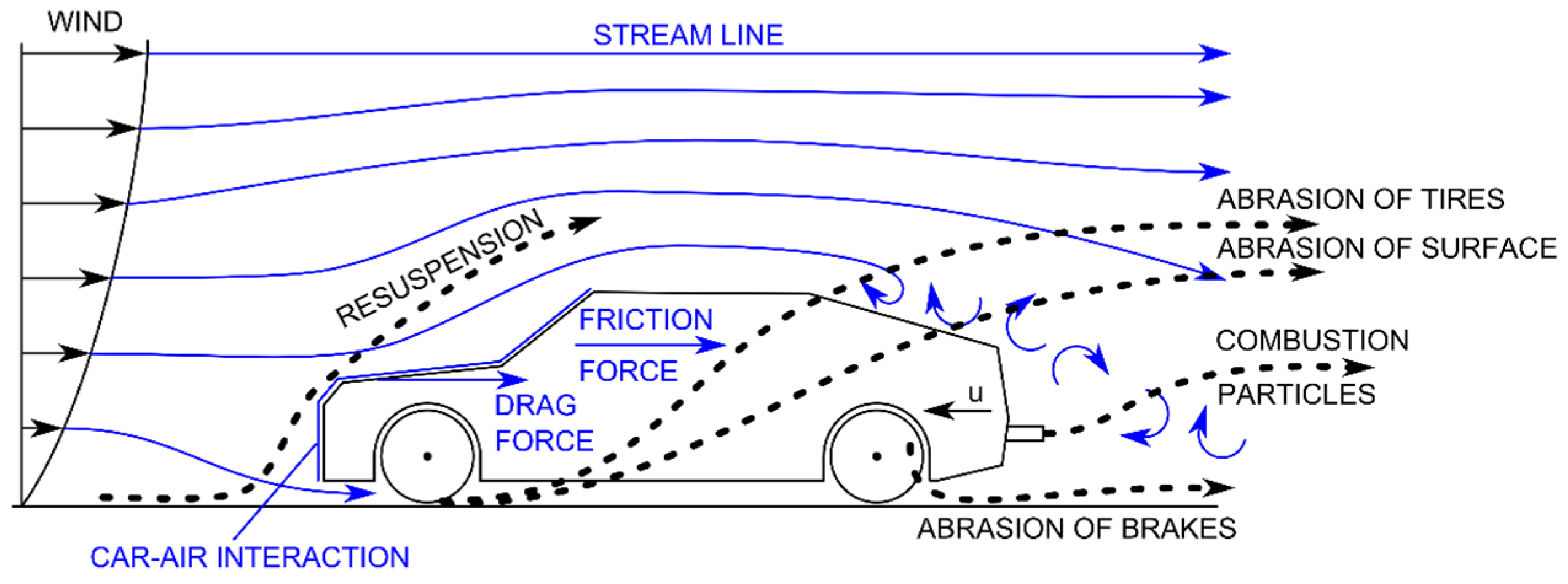
1. Introduction
2. Numerical Model
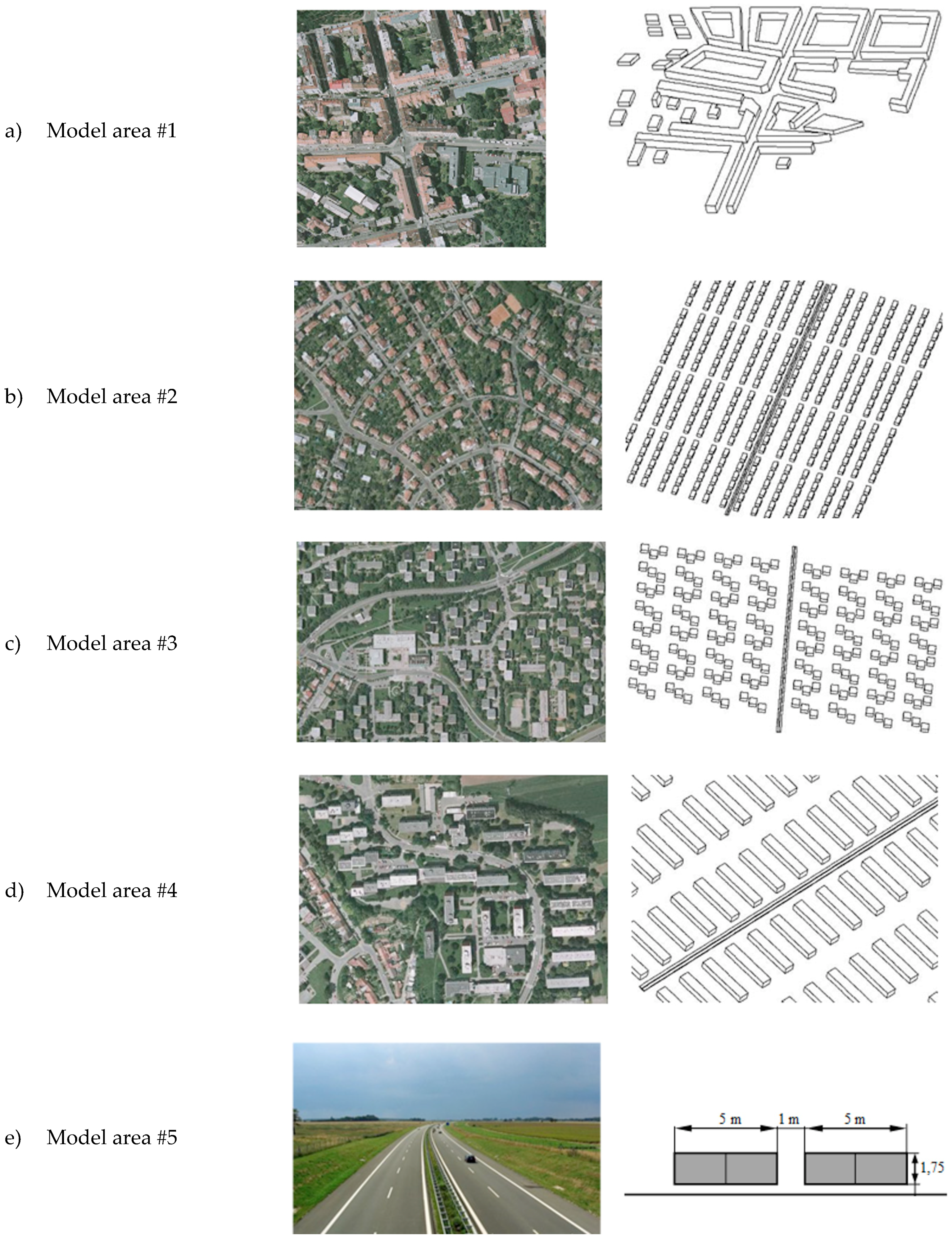
2.1. Built-Up Area Geometries
- Model area #1: An intersection located in an urban center: a crossing of two roads that pass through a built-up area comprising lines of four-story houses (a concrete geometry from the central district of Brno).
- Model area #2: A road passing through a residential area with single-family houses; the 10-m-high units are positioned with a spacing of 15 m, the ground plan of each home equals 10 × 15 m2, six houses in a row form a regular block of buildings, there is a 15-m-wide aisle (perpendicular to the main road) separating individual blocks of houses, and 20-m-wide service roads parallel to the main road run through the urban area every two rows of houses.
- Model area #3: A road running between small-size prefabricated houses positioned at regular intervals and having the dimensions of of 20 × 20 × 20 m2. The buildings are arranged into separate groups, each of which contains three closely neighboring units.
- Model area #4: A road passing through an area containing prefabricated houses configured into longitudinally oriented 15-m-high blocks that are positioned at regular intervals of 50 m and invariably exhibit the ground plan dimensions of 17 × 90 m2.
- Model area #5: A road in a free space: an almost ideally straight road running through an open landscape, with no barriers in the immediate vicinity. This model item is included to compare the built-up and the open-space pollutant dispersion scenarios.
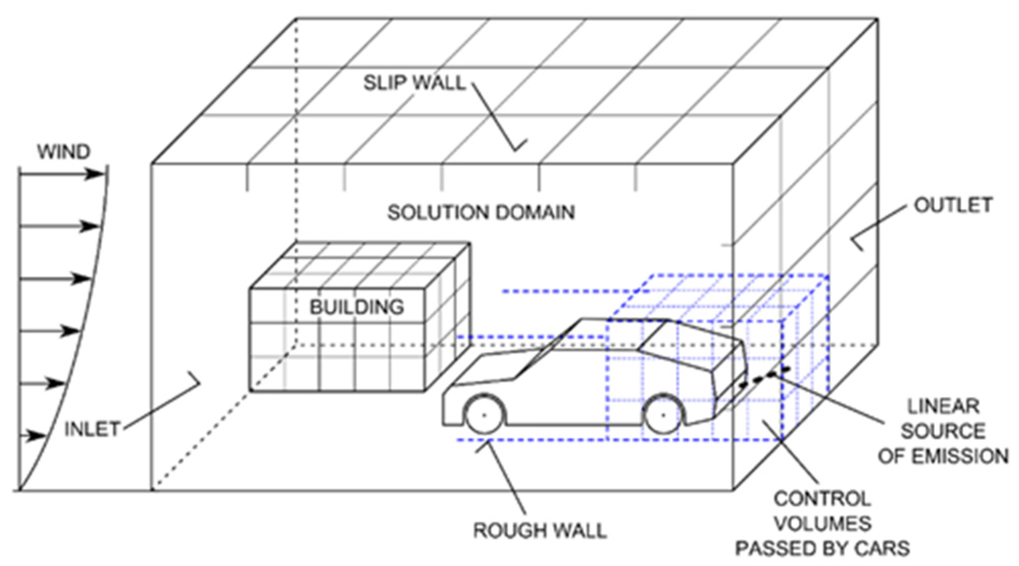
2.2. Mathematical Description and Boundary Conditions
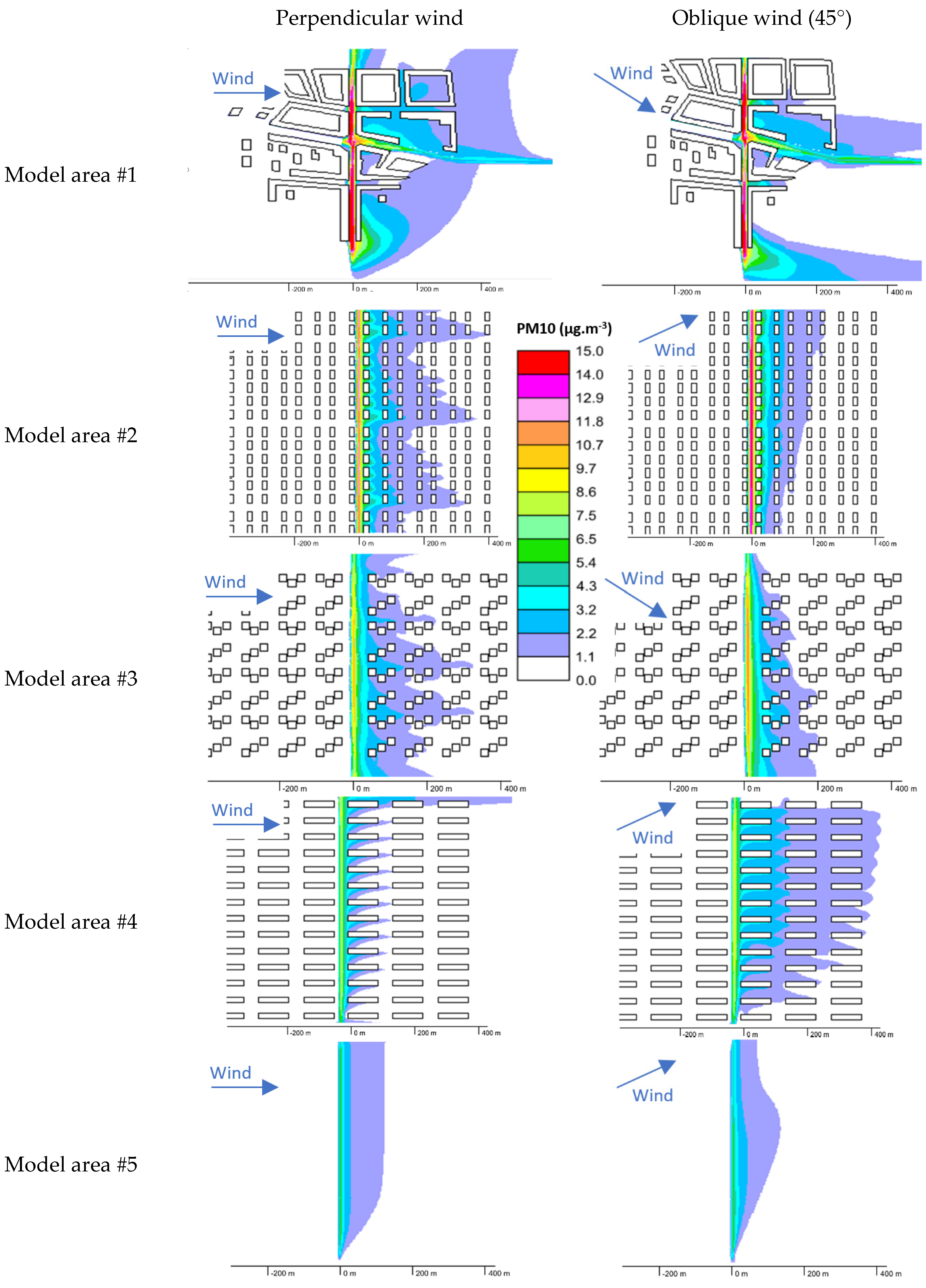
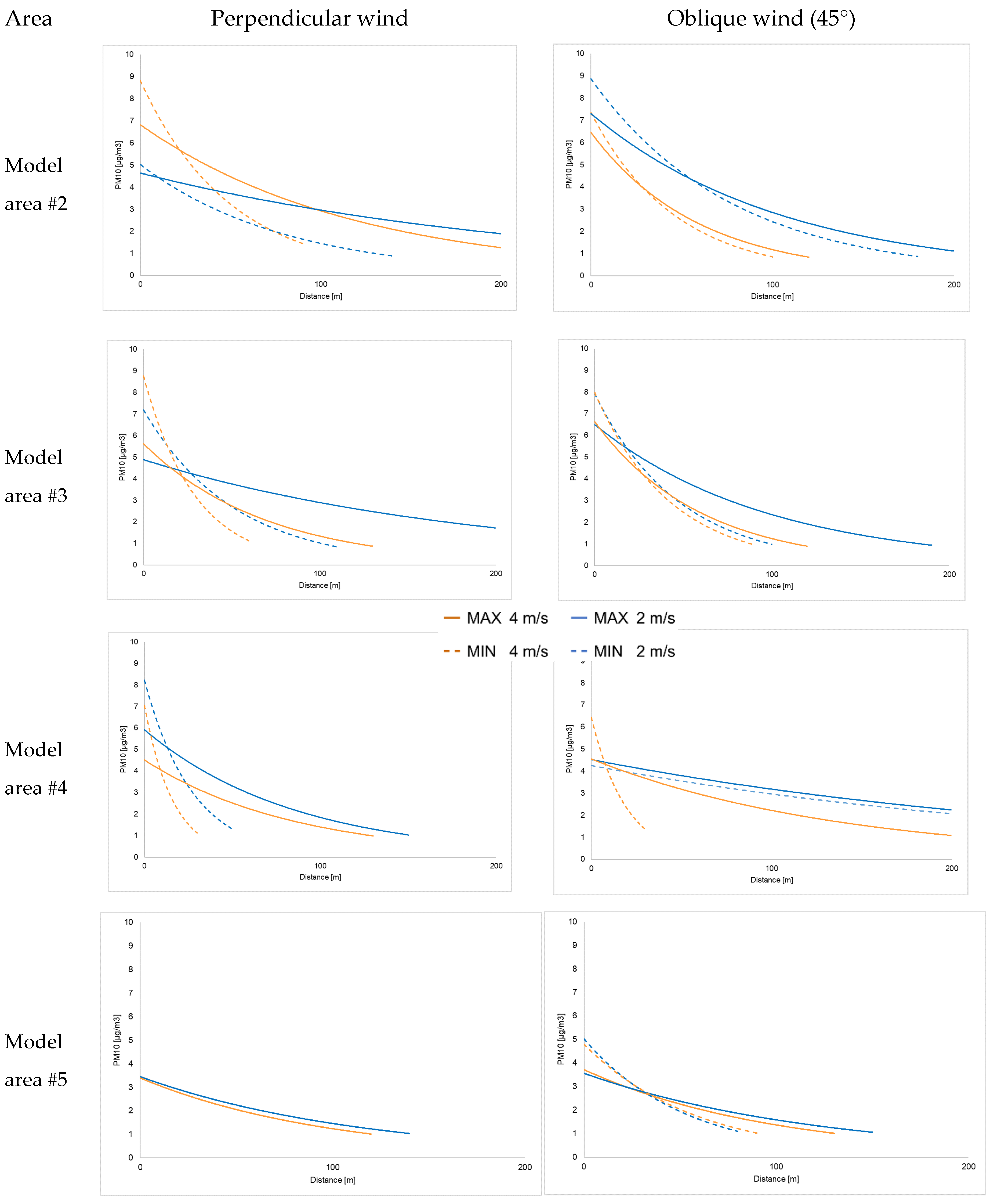
2.3. Numerical Simulation Results
3. Generalizing the Results
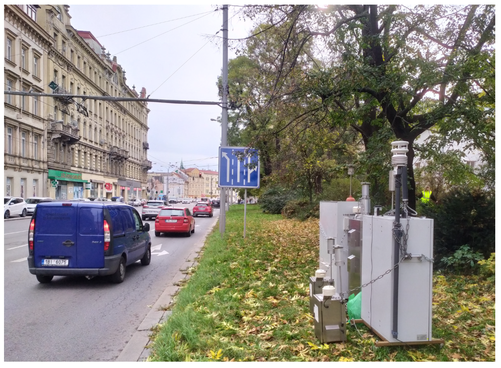
4. Comparing the Numerical Prediction with the In-Situ Measurements
5. Conclusions
Author Contributions
Funding
Conflicts of Interest
References
- Santibáñez-Andrade, M.; Quezada-Maldonado, E.M.; Osornio-Vargas, Á.; Sánchez-Pérez, Y.; García-Cuellar, C.M. Air pollution and genomic instability: The role of particulate matter in lung carcinogenesis. Environ. Pollut. 2017, 229, 412–422. [Google Scholar] [CrossRef] [PubMed]
- Appel, J.; Bockhorn, H.; Frenklach, M. Kinetic modeling of soot formation with detailed chemistry and physics: Laminar premixed flames of C2 hydrocarbons. Combust. Flame 2000, 121, 122–136. [Google Scholar] [CrossRef]
- Jicha, M.; Katolicky, J.; Pospisil, J. Dispersion of pollutants in a street canyon and street intersection under traffic-induced flow and turbulence using a low Re κ-ε model. Int. J. Environ. Pollut. 2002, 18, 160–170. [Google Scholar] [CrossRef]
- Jiang, Y.-Q.; Ma, P.-J.; Zhou, S.-G. Macroscopic modeling approach to estimate traffic-related emissions in urban areas. Transp. Res. Part D Transp. Environ. 2018, 60, 41–55. [Google Scholar] [CrossRef]
- Tissari, J.; Hytönen, K.; Sippula, O.; Jokiniemi, J. The effects of operating conditions on emissions from masonry heaters and sauna stoves. Biomass Bioenergy 2009, 33, 513–520. [Google Scholar] [CrossRef]
- Pospisil, J.; Katolicky, J.; Jicha, M. A comparison of measurements and CFD model predictions for pollutant dispersion in cities. Sci. Total Environ. 2004, 334–335, 185–195. [Google Scholar] [CrossRef] [PubMed]
- Holmes, N.S.; Morawska, L. A review of dispersion modelling and its application to the dispersion of particles: An overview of different dispersion models available. Atmos. Environ. 2006, 40, 5902–5928. [Google Scholar] [CrossRef]
- Woodward, H.; Stettler, M.; Pavlidis, D.; Aristodemou, E.; ApSimon, H.; Pain, C. A large eddy simulation of the dispersion of traffic emissions by moving vehicles at an intersection. Atmos. Environ. 2019, 215, 116891. [Google Scholar] [CrossRef]
- Zhang, Y.; Gu, Z.; Wah Yu, C. Large eddy simulation of vehicle induced turbulence in an urban street canyon with a new dynamically vehicle-tracking scheme. Aerosol Air Qual. Res. 2017, 17, 865–874. [Google Scholar] [CrossRef]
- Shen, J.; Gao, Z.; Ding, W.; Yu, Y. An investigation on the effect of street morphology to ambient air quality using six real-world cases. Atmos. Environ. 2017, 164, 85–101. [Google Scholar] [CrossRef]
- Zhang, X.; Zhang, Z.; Su, G.; Tao, H.; Xu, W.; Hu, L. Buoyant wind-driven pollutant dispersion and recirculation behaviour in wedge-shaped roof urban street canyons. Environ. Sci. Pollut. Res. 2019, 26, 8289–8302. [Google Scholar] [CrossRef] [PubMed]
- Miao, C.; Yu, S.; Hu, Y.; Bu, R.; Qi, L.; He, X.; Chen, W. How the morphology of urban street canyons affects suspended particulate matter concentration at the pedestrian level: An in-situ investigation. Sustain. Cities Soc. 2020, 55, 102042. [Google Scholar] [CrossRef]
- Auguste, F.; Lac, C.; Masson, V.; Cariolle, D. Large-eddy simulations with an immersed boundary method: Pollutant dispersion over urban terrain. Atmosphere 2020, 11, 113. [Google Scholar] [CrossRef]
- Eskridge, R.E.; Hunt, J.C. Highway modeling. Part I: Prediction of velocity and turbulence fields in the wake of vehicles. J. Appl. Meteor. 1979, 18, 387–400. [Google Scholar] [CrossRef]
- Sedefian, L.; Trivikrama Rao, S.; Czapski, U. Effects of traffic-generated turbulence on near-field dispersion. Atmos. Environ. (1967) 1981, 15, 527–536. [Google Scholar] [CrossRef]
- Sini, J.-F.; Mestayer, P.G. Traffic-induced urban pollution: A numerical simulation of street dispersion and net production. In Air Pollution Modeling and Its Application XII; Springer: Boston, MA, USA, 1998; pp. 369–377. [Google Scholar]
- EMEP/EEA Air Pollutant Emission Inventory Guidebook 2019. Available online: https://www.eea.europa.eu/publications/emep-eea-guidebook-2019/part-b-sectoral-guidance-chapters/1-energy/1-a-combustion/1-a-3-b-i/view (accessed on 30 March 2020).
- Labovský, J.; Jelemenský, L. Verification of CFD pollution dispersion modelling based on experimental data. J. Loss Prev. Process Ind. 2011, 24, 166–177. [Google Scholar] [CrossRef]
- Tsai, M.Y.; Chen, K.S. Measurement and three-dimensional modeling of air pollutant dispersion in an urban street canyon. Atmos. Environ. 2004, 38, 5911–5924. [Google Scholar] [CrossRef]


| Car Type | PV | LCV | HDV | UB | Share of Car Types According to Emission Standards (%) | |||||||
|---|---|---|---|---|---|---|---|---|---|---|---|---|
| Fuel | Petrol | Diesel | Petrol | Diesel | Diesel | Diesel | NG | PC | LCV | HDV | UB | |
| Emission standards | PRE ECE | 0.0032 | 0.2164 | 0.0032 | 0.2493 | 0.5671 | 0.7636 | 0.0200 | 0.9 | 0.3 | 5.5 | 0 |
| Euro 1 | 0.0032 | 0.0569 | 0.0032 | 0.0903 | 0.4021 | 0.3635 | 0.0100 | 4.1 | 2.9 | 1.3 | 10.5 | |
| Euro 2 | 0.0032 | 0.0467 | 0.0032 | 0.0903 | 0.1772 | 0.1830 | 0.0100 | 9.4 | 4.5 | 6.5 | 15.8 | |
| Euro 3 | 0.0012 | 0.0310 | 0.0012 | 0.0662 | 0.2078 | 0.1817 | 0.0095 | 21.6 | 24.5 | 30.9 | 26.3 | |
| Euro 4 | 0.0012 | 0.0316 | 0.0012 | 0.0356 | 0.0429 | 0.0458 | 0.0095 | 29.1 | 49.7 | 20.9 | 36.8 | |
| Euro 5 | 0.0015 | 0.0027 | 0.0015 | 0.0027 | 0.0527 | 0.0519 | 0.0095 | 29.5 | 15.8 | 24.9 | 5.3 | |
| Euro 6 | 0.0018 | 0.00199 | 0.0018 | 0.0019 | 0.0058 | 0.0051 | 0.0095 | 5.4 | 2.2 | 10 | 5.3 | |
| Share of cars according to fuel [%] | 45.84 | 54.16 | 13.52 | 86.48 | 100.00 | 46.67 | 53.33 | |||||
| Emission Factors Weighted with Shares of Fuel and Car Types (g·km−1) | ||||||||||||
| Emission standards | PRE ECE | 0.0010 | 0.0006 | 0.0312 | 0.0000 | |||||||
| Euro 1 | 0.0013 | 0.0022 | 0.0052 | 0.0183 | ||||||||
| Euro 2 | 0.0025 | 0.0035 | 0.0115 | 0.0143 | ||||||||
| Euro 3 | 0.0037 | 0.0140 | 0.0642 | 0.0236 | ||||||||
| Euro 4 | 0.0051 | 0.0154 | 0.0089 | 0.0097 | ||||||||
| Euro 5 | 0.0006 | 0.0004 | 0.0131 | 0.0015 | ||||||||
| Euro 6 | 0.0001 | 0.0001 | 0.0005 | 0.0004 | Aggregate Emission factor (g·km−1) | |||||||
| Summary emission factors | 0.0146 | 0.0364 | 0.1349 | 0.0680 | 0.2538 | |||||||
| Wind Direction | Area | Velocity (m·s−1) | Range | a | b | R2 |
|---|---|---|---|---|---|---|
| 90° | #2 | 4 | MAX | 6.831 | −0.008 | 0.983 |
| MIN | 4.641 | −0.004 | 0.863 | |||
| 2 | MAX | 8.821 | −0.020 | 0.940 | ||
| MIN | 5.027 | −0.012 | 0.808 | |||
| #3 | 4 | MAX | 5.629 | −0.014 | 0.881 | |
| MIN | 8.773 | −0.034 | 0.979 | |||
| 2 | MAX | 4.888 | −0.005 | 0.870 | ||
| MIN | 7.201 | −0.019 | 0.905 | |||
| #4 | 4 | MAX | 4.516 | −0.012 | 0.932 | |
| MIN | 7.064 | −0.061 | 0.985 | |||
| 2 | MAX | 5.922 | −0.012 | 0.981 | ||
| MIN | 8.227 | −0.037 | 0.955 | |||
| #5 | 4 | MAX | 3.399 | −0.010 | 0.944 | |
| 2 | MAX | 3.455 | −0.009 | 0.872 | ||
| 45° | #2 | 4 | MAX | 6.465 | −0.017 | 0.863 |
| MIN | 7.369 | −0.022 | 0.907 | |||
| 2 | MAX | 7.311 | −0.009 | 0.885 | ||
| MIN | 8.879 | −0.013 | 0.942 | |||
| #3 | 4 | MAX | 6.637 | −0.017 | 0.916 | |
| MIN | 7.987 | −0.024 | 0.969 | |||
| 2 | MAX | 6.504 | −0.010 | 0.945 | ||
| MIN | 7.931 | −0.021 | 0.958 | |||
| #4 | 4 | MAX | 4.555 | −0.007 | 0.989 | |
| MIN | 6.449 | −0.052 | 0.854 | |||
| 2 | MAX | 4.525 | −0.004 | 0.950 | ||
| MIN | 4.254 | −0.004 | 0.916 | |||
| #5 | 4 | MAX | 3.716 | −0.010 | 0.921 | |
| MIN | 4.794 | −0.017 | 0.982 | |||
| 2 | MAX | 3.559 | −0.008 | 0.901 | ||
| MIN | 5.024 | −0.019 | 0.991 |
| Wind Direction | Wind Velocity | PM10 In-Situ Measurement | PM10 Numerical Prediction | Comparison | |||
|---|---|---|---|---|---|---|---|
| Measured Concentration Recalculated to Specific Traffic Intensity | Background Contribution | Road Contribution | Road Contribution MAX | Road Contribution MIN | Experiment/Prediction Ration | ||
| (μg·m−3) | (μg·m−3) | (μg·m−3) | (μg·m−3) | (μg·m−3) | (-) | ||
| perpendicular | 2 m·s−1 | 53.27 | 48.00 | 5.27 | 10.13 | 8.33 | 52% |
| perpendicular | 4 m·s−1 | 48.36 | 43.58 | 4.79 | 9.20 | 8.33 | 55% |
| oblique (45°) | 2 m·s−1 | 55.71 | 42.00 | 13.71 | 15.80 | 10.07 | 136% |
| oblique (45°) | 4 m·s−1 | 31.13 | 23.47 | 7.66 | 12.60 | 8.60 | 89% |
© 2020 by the authors. Licensee MDPI, Basel, Switzerland. This article is an open access article distributed under the terms and conditions of the Creative Commons Attribution (CC BY) license (http://creativecommons.org/licenses/by/4.0/).
Share and Cite
Pospisil, J.; Huzlik, J.; Licbinsky, R.; Spilacek, M. Dispersion Characteristics of PM10 Particles Identified by Numerical Simulation in the Vicinity of Roads Passing through Various Types of Urban Areas. Atmosphere 2020, 11, 454. https://doi.org/10.3390/atmos11050454
Pospisil J, Huzlik J, Licbinsky R, Spilacek M. Dispersion Characteristics of PM10 Particles Identified by Numerical Simulation in the Vicinity of Roads Passing through Various Types of Urban Areas. Atmosphere. 2020; 11(5):454. https://doi.org/10.3390/atmos11050454
Chicago/Turabian StylePospisil, Jiri, Jiri Huzlik, Roman Licbinsky, and Michal Spilacek. 2020. "Dispersion Characteristics of PM10 Particles Identified by Numerical Simulation in the Vicinity of Roads Passing through Various Types of Urban Areas" Atmosphere 11, no. 5: 454. https://doi.org/10.3390/atmos11050454
APA StylePospisil, J., Huzlik, J., Licbinsky, R., & Spilacek, M. (2020). Dispersion Characteristics of PM10 Particles Identified by Numerical Simulation in the Vicinity of Roads Passing through Various Types of Urban Areas. Atmosphere, 11(5), 454. https://doi.org/10.3390/atmos11050454