Article

The Influence of Meteorology and Air Transport on CO2 Atmospheric Distribution over South Africa

by
Xolile G. Ncipha
1,2,*,
Venkataraman Sivakumar
2 and
Oupa E. Malahlela
3
1
South African Weather Service, Private Bag X097, Pretoria 0001, South Africa
2
School of Chemistry and Physics, University of KwaZulu-Natal, Durban 4000, South Africa
3
Department of Ecology and Resource Management, School of Environmental Sciences, University of Venda, Thohoyandou 0950, South Africa
*
Author to whom correspondence should be addressed.
Atmosphere 2020, 11(3), 287; https://doi.org/10.3390/atmos11030287
Submission received: 8 November 2019 / Revised: 28 February 2020 / Accepted: 2 March 2020 / Published: 16 March 2020
(This article belongs to the Section Meteorology)

Abstract

:
This paper demonstrates the role of meteorology and air transport in influencing the South African atmospheric CO2 distribution. CO2 data from December 2004 to December 2009 acquired by the Tropospheric Emission Spectrometer (TES) instrument onboard the Aura satellite were used to establish the CO2 vertical distribution at selected regions in South Africa. The Hybrid Single-Particle Lagrangian Integrated Trajectories (HYSPLIT) atmospheric model backward trajectories were used to determine the long-range air transport impacting on South African CO2 atmospheric distribution and to detect the source areas of air masses impacting on South Africa’s atmosphere. The study found that long-range air transport can result in the accumulation or dilution of atmospheric CO2 at various sites in South Africa, depending on the source region and type of air flow. The long-range air transport from different source regions at the upper air level between the 700 and 500 hPa stable layers and the layer above 500 hPa strengthens the inhomogeneity in the vertical distribution of CO2, which is caused by the decoupling effect of the upper air stable layers. This long-range air transport also involves intercontinental air transport.

1. Introduction

Free troposphere and stratospheric CO2 is a long-lived greenhouse gas (LLGHG), which is an effective tracer of atmospheric dynamics and transport in these layers. It has an atmospheric lifetime of 50 to 200 years [1,2] and contributes about 66% of the gaseous radiative forcing responsible for anthropogenic climate change. Among the LLGHGs, CO2 increases have caused the largest sustained radiative forcing over the past decade [1,3,4,5,6,7,8,9]. The atmospheric CO2 mixing ratio is controlled by processes such as natural and anthropogenic emissions, chemical transformation, wet scavenging, surface uptake by terrestrial and ocean ecosystems, and transport at different scales [5,10]. Since the industrial revolution, the increases in global atmospheric CO2 are due to anthropogenic activities, particularly dominated by emissions from the combustion of fossil fuel, gas flaring, and cement production. Other sources include emissions due to land use changes such as deforestation and biomass burning [1,3,4,7,8,9,10,11].
Several studies have been undertaken in the Southern Hemisphere to investigate the influence of atmospheric dynamics and transport on the distribution of atmospheric constituents, mainly air pollutants, at the surface and middle troposphere [12,13,14,15,16,17,18,19,20]. Throughout much of the year, Southern Africa and the adjacent Atlantic and Indian Oceans are located in the region of planetary-scale subsidence occurring between the Hadley and Ferrel cells of the Southern Hemisphere general circulation. The atmospheric circulation is characterized by the regular occurrence of semi-permanent, subtropical anticyclones, which occur between the latitudes 15° and 35° S, over eastern South America, the Atlantic Ocean, the African continent, and the Indian Ocean. These high-pressure systems result in three widespread and temporal persistent stable discontinuities that frequently occur in the vertical structure of the atmosphere. The first discontinuity occurs at the top of the mixing layer and is centered at 700 hPa (3000 m.a.s.l.); the second is associated with the main subsidence inversion located at about 500 hPa level (5000 m.a.s.l), and the third was at about 350 hPa level (8000 m.a.s.l.), bounded below and above by the 500 hPa level subsidence and tropopause, respectively. On some days, the mixed layer can be deeper and extend up to 500 hPa, after the 700 hPa discontinuity has been broken by the passage of the convective westerly wave disturbance. The 500 hPa discontinuity is temporally persistent and can withstand the passage of shallow westerly disturbances [12,13]. The result of this temporal persistence of multiple stable layers is the trapping of surface originating pollutants into altitude bands of air pollution, and the limitation of vertical transport [13,14,18]. However, well developed deep low-pressure troughs and cut off low (COL) pressure systems can destabilize the whole column of the troposphere up to the stratosphere. This enables air mass transfer between the troposphere and stratosphere [13,18,21]. In the Southern Hemisphere, the COLs occur in the midlatitudes to subtropics and around the three main continental areas: Australia, Southern Africa, and South America. Their density of occurrence is greatest at 300 hPa atmospheric level, followed by 500 hPa, and the minimum is at 200 hPa. The occurrence of COLs at these atmospheric levels have a seasonal variability, with peaks in summer, autumn, and winter at 200, 300 and 500 hPa, respectively [22].
The transport of an air mass at a particular location is based on the circulation type prevailing at the location of the origin of the transport. Transportation of air pollutants from biomass burning products, urban and industrial emissions in the troposphere from the Southern Hemisphere continents is driven by interacting planetary and synoptic scale features of the general circulation of the Southern Hemisphere. The South Atlantic anticyclonic circulation is responsible for the intercontinental transport between Southern Africa and South America. In Southern Africa, the continental air mass exits the subcontinent over the west coast into the South Atlantic Ocean, driven by easterly waves [12,13,15]. This African air mass is then carried northwesterly, then easterly, to the northern part of South America under the influence of the South Atlantic anticyclone, then turns southward on the western edge of the Atlantic anticyclonic circulation, which overlaps the South American land mass, and ends up re-crossing the Atlantic Ocean in an easterly direction at higher southern latitudes toward Southern Africa [16,17,19,20]. During the dry season, which spans from June to October, the recirculated air is entrained by biomass fire emissions from the Amazon Basin, resulting in polluted air that is advected to Southern Africa at high altitudes [16,17,19,20,23,24,25,26]. Marenco et al. [26] observed layers of biomass emissions of high loading at elevated altitudes that extended from 1–1.5 to 4–6 km at the Amazon Basin. Edwards et al. [17] observed high carbon monoxide mixing ratio values of about 180 ppb in air masses transported from South America to Southern Africa at 700 hPa. Over Southern Africa, air mass transport is controlled by four major circulation types, which have an annual cycle: the semi-permanent subtropical anticyclones; transient mid-latitude ridging anticyclones; westerly baroclinic disturbances; and barotropic quasi-stationary tropical easterly waves [12,13,14].
Though South Africa is the dominant source region of fossil fuel emissions in Southern Africa [27,28], the country has been understudied with regard to CO2 atmospheric distribution. A recent study was undertaken in Cape Town city to estimate CO2 emissions by inverse modeling [29]. This study illustrates how the climatology of circulation patterns and the air transport influenced the CO2 atmospheric distribution in South Africa. Air mass source regions that impacted the South African CO2 atmospheric mixing ratios at different levels of the atmosphere have also been identified. More recently, Ncipha and Sivakumar [30] conducted preliminary investigations on the influence of meteorology and air transport on South African atmospheric CO2 distribution during the summer and winter seasons.

2. Materials and Methods

2.1. CO2 Analysis

2.1.1. Tropospheric Emission Spectrometer (TES) Instrument

This study used CO2 level 2 data collected from the Tropospheric Emission Spectrometer (TES) instrument onboard the Aura satellite. The objective of the TES is to make comprehensive global stratospheric and tropospheric composition measurements from the four instruments onboard. TES is an infrared, high-resolution Fourier transform spectrometer (FTS) and operates in both nadir (downward view) and limb (side view) modes to measure the vertical distribution of the atmospheric composition and surface parameters [31,32,33,34,35,36,37,38,39]. The CO2 profile data were produced by the National Aeronautics and Space Administration (NASA) and made accessible from the TES website https://tes.jpl.nasa.gov/data.

2.1.2. Ground Station CO2 Data

The ground CO2 data were monitored from the Global Atmosphere Watch (GAW) station at Cape Point, located at the southern end of Cape Peninsula, South Africa (34.35° S, 18.49° E). The Cape Point GAW station is a member of the GAW global network. The station is exposed to the sea, on top of a cliff 230 m in altitude. The Cape Point station is predominantly impacted by the on-shore flow from the South Atlantic Ocean and is representative of southern hemispheric background conditions [29,40]. The CO2 has been monitored continuously using a non-dispersive infra-red (NDIR) instrument since 1993, and the CO2 sampling flask program started in 2010 [41]. The GAW Cape Point station CO2 data were provided directly from the station and is also available at the World Data Center for Greenhouse Gases (WDCGG) website https://gaw.kishou.go.jp.

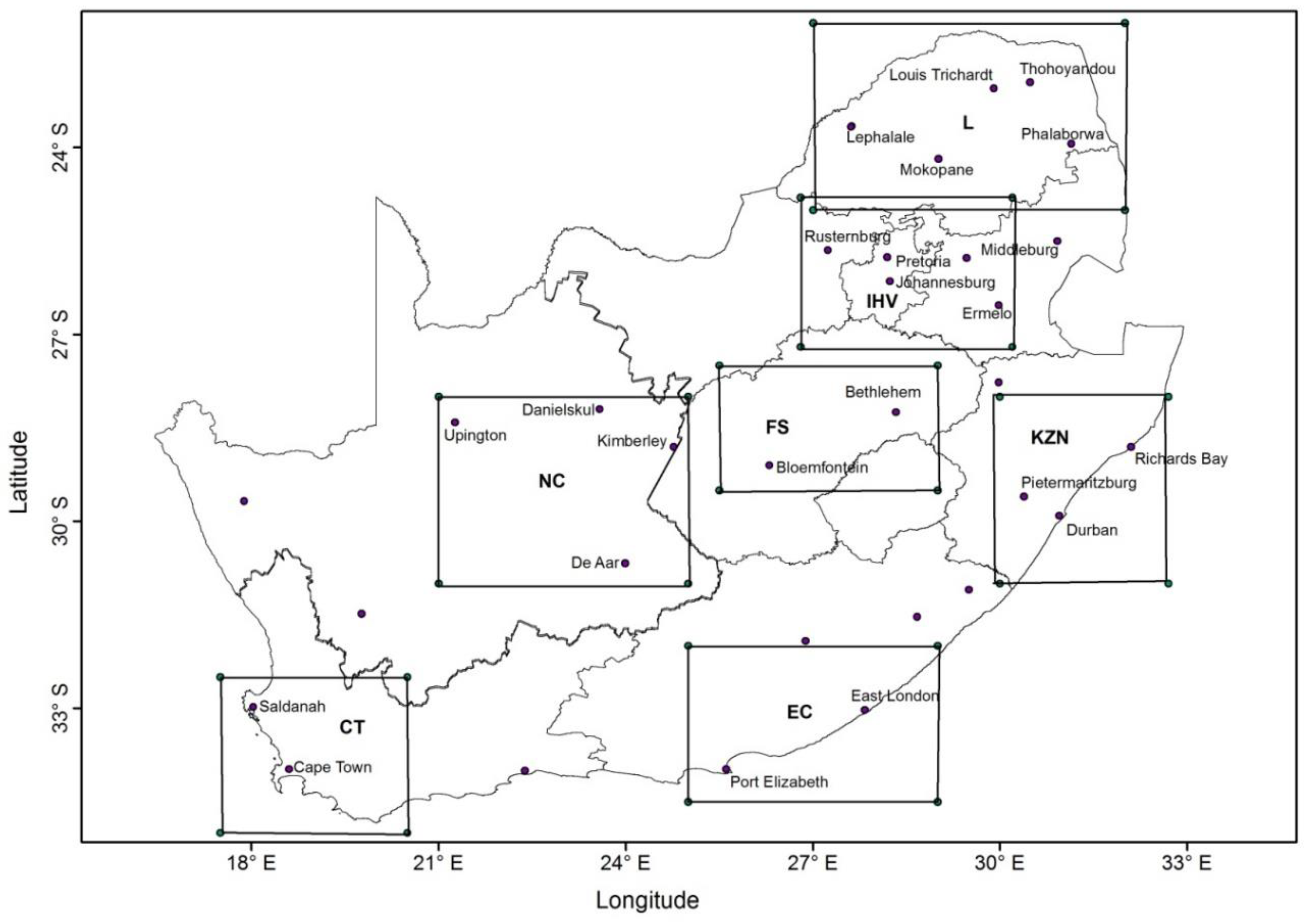
2.1.3. CO2 Study Region Locations and Description

The analysis involved the TES nadir view data within the South African domain, bounded by the (17° to 33°) E longitude and (22° to 35°) S latitude. Seven areas of interest within South Africa were chosen to characterize the seasonal vertical distribution of CO2. Table 1 and Figure 1 show the areas and their demarcations. The boundaries of these study regions were chosen to include urbanized and industrialized towns and rural towns.
The Cape Town (CT) study region is located at the southwest coast of the country. It extends from the southwest coast into the interior of Western Cape Province including the City of Cape Town and other towns within the province (Figure 1). Cape Town city is the economic hub of the province and has several industrial areas. This study area also included a dense and diverse biome [42].
The central Free State (FS) area lies at the center of the country and overlaps the northwestern part of Lesotho (Figure 1). The landscape of this area is dominated by agricultural activities; it is mainly cultivated land and natural savanna grassland. Gold mining is an important industrial activity in the study area [42].
The central Northern Cape (NC) (Karoo) area was selected because it is a national terrestrial background area. The national spatial industrial CO2 source inventory from Osman et al. [43] indicates only one industrial CO2 emitter in the area, which is a large iron-ore mine [42]. The NC is a semiarid area, as a result it experiences a lack of biomass fire emissions [44,45].
The Eastern Cape (EC) study area lies on the southeast coast of the country. It encompasses the two metropolitan towns, East London and Port Elizabeth, surrounding small towns, and dense bushland. The area has a diverse natural biome. East London and Port Elizabeth have major harbors and both of them are in the vicinity of the industrial complexes in both cities. The automotive industry is an important sector in the economy of both of these cities [42].
The KwaZulu-Natal (KZN) study area lies on the east coast of the country. It includes the three cities Durban, Pietermaritzburg, and Richards Bay, small surrounding towns, nature reserves, and forests. The major CO2 emitting industries in this area are agriculture, forestry, aluminum, petrochemicals, steel production, paper and board manufacturing, automotive manufacturing, and a range of industries linked with imports and exports at the major ports in Durban and Richards Bay [42]. Another important source of CO2 in KZN is its leakage from groundwater wells. Several sites at the Bongwana village (south of KZN) have been identified and monitored for ground CO2 leakages [46].
The Industrial Highveld (IHV) study area has the largest concentration of industrial infrastructure [47]. Osman et al. [43] indicated that this region had the highest concentration of industrial CO2 emitters. Rustenburg and Brits towns in the IHV produce 94% of South Africa’s platinum and have the largest reserves of this mineral in the world. The IHV area has urban-industrial complexes situated in Johannesburg, Vaal Triangle, and Pretoria city. The IHV region is rich in coal reserves, with Witbank town, now renamed eMalahleni, being the largest coal producer in Africa. The abundance of coal and other mineral resources in this region has led to the development of the region into one of the major industrial and urban population centers of South Africa. As a result, the area is the major power generating region of the country, with 11 large coal-generating power plants and the domestic fossil fuel burning emissions are also important contributors to emissions in this region [42,48,49].
The Limpopo Province (L) study area is located in the northern most part of South Africa, sharing borders with Mozambique, Zimbabwe, and Botswana (Figure 1). The landscape of this province is dominated by mixed grassland and trees. Agriculture is an important sector in the provincial economy. Limpopo is also rich in mineral resources, resulting in mining and other related industries being important contributors in this province’s economy. Phalaborwa and Thabazimbi are Limpopo’s major mining centers [42]. The province houses two dry-cooled coal-fired power stations called Matimba and Medupi. Matimba is located in a town called Lephalale and Medupi is just to its west. The Matimba power station was designed to generate 4000 MW and was ranked the largest direct dry-cooled power station in the world. The recently commissioned Medupi power station, which is not operated at its full capacity, is designed to generate 4764 MW [50].

2.1.4. CO2 Data Analysis

The TES nadir view surface level (approximately 1000 hPa) CO2 data were compared with the ground-based Cape Point GAW station data. The two datasets were compared when the TES data was within 0.5° (approximately 50 km) latitude and longitude radius from the ground station. This distance was chosen as a maximum practical distance between the two datasets in order to reduce the possibilities of these two measurement platforms sampling different air masses. This relatively long distance is a compromise for the spatial representativeness of GAW data in preference to obtaining enough of a sample size of the TES data for a fair comparison of the two datasets. The best opportunity for sampling spatially homogeneously mixed air is when the GAW station is impacted by southerly on-shore maritime airflow [51]. The validation requirements for satellite-based atmospheric CO2 measurements with ground-based observations vary depending on the spatial and temporal variability of atmospheric CO2 [39]. Kulawik et al. [39] found a bias of TES against aircraft CO2 data to be within 1 ppm for all pressure levels. The comparison period was from 23/05/2005 to 28/03/2008 and the satellite overpasses were centered at 13:00 (GMT), which satisfied the chosen coincidence (spatial comparison) criteria. The 30 min averaged 13:00 (GMT) data from the GAW station were used for the comparisons.
The TES CO2 data were analyzed from December 2004 to December 2009, after that period, the instrument scans became less frequent and irregular. Averaged CO2 vertical profiles in the study regions (Figure 1) were constructed by averaging atmospheric CO2 horizontally at the same altitude. The averaging was computed from the ground level up to 18 km altitude into the lower stratosphere during the austral summer (DJF) 2004–2009, autumn (MAM) 2005–2009, winter (JJA) 2005–2009, and spring (SON) 2005–2009 seasons. The tropopause in the subtropics of the Southern Hemisphere varies between 15 and 16 km, its seasonal minimum altitude is during the winter [52]. The CO2 data were not subjected to de-trending analysis because of the short study period (five years) and low frequency of the satellite sampling scans (near same location observations were repeated on a cycle every 16 days). This may subject the data to some seasonal bias due to the CO2 long-term increasing trend, as the seasonal difference may not be purely due to seasonal dynamics.

2.2. Atmospheric Circulation Analysis

This study used reanalysis data from the National Centers for Environmental Prediction (NCEP) and National Center for Atmospheric Research (NCAR) to establish a 5-year seasonal climatology of circulation patterns over Southern Africa, the South Atlantic, and Indian Ocean. The reanalysis data are the product of a collaborative project between the NCEP and NCAR to produce records of the global analyses of atmospheric fields in 17 standard pressure levels in support of the atmospheric science community. The project involves the collection of atmospheric data from various observation platforms, then quality controlling and assimilating it [53]. This study produced a 5-year seasonal climatology of circulation patterns from the National Oceanic and Atmospheric Administration/Earth System Research Laboratory’s Physical Sciences Division (NOAA/ESRL: PSD) website http://www.esrl.noaa.gov/psd/. The seasonal circulation patterns were derived from 5-year averages of geopotential heights computed by the system at the 1000, 700, and 500 hPa pressure levels for austral summer (DJF) 2004–2009, autumn (MAM) 2005–2009, winter (JJA) 2005–2009, and spring (SON) 2005–2009. The study domains for the geopotential height field were (0° to 50° E) and (0° to 40° S) at 1000 hPa and (50° W to 40° E) and (0° to 40° S) at 700 hPa and 500 hPa.

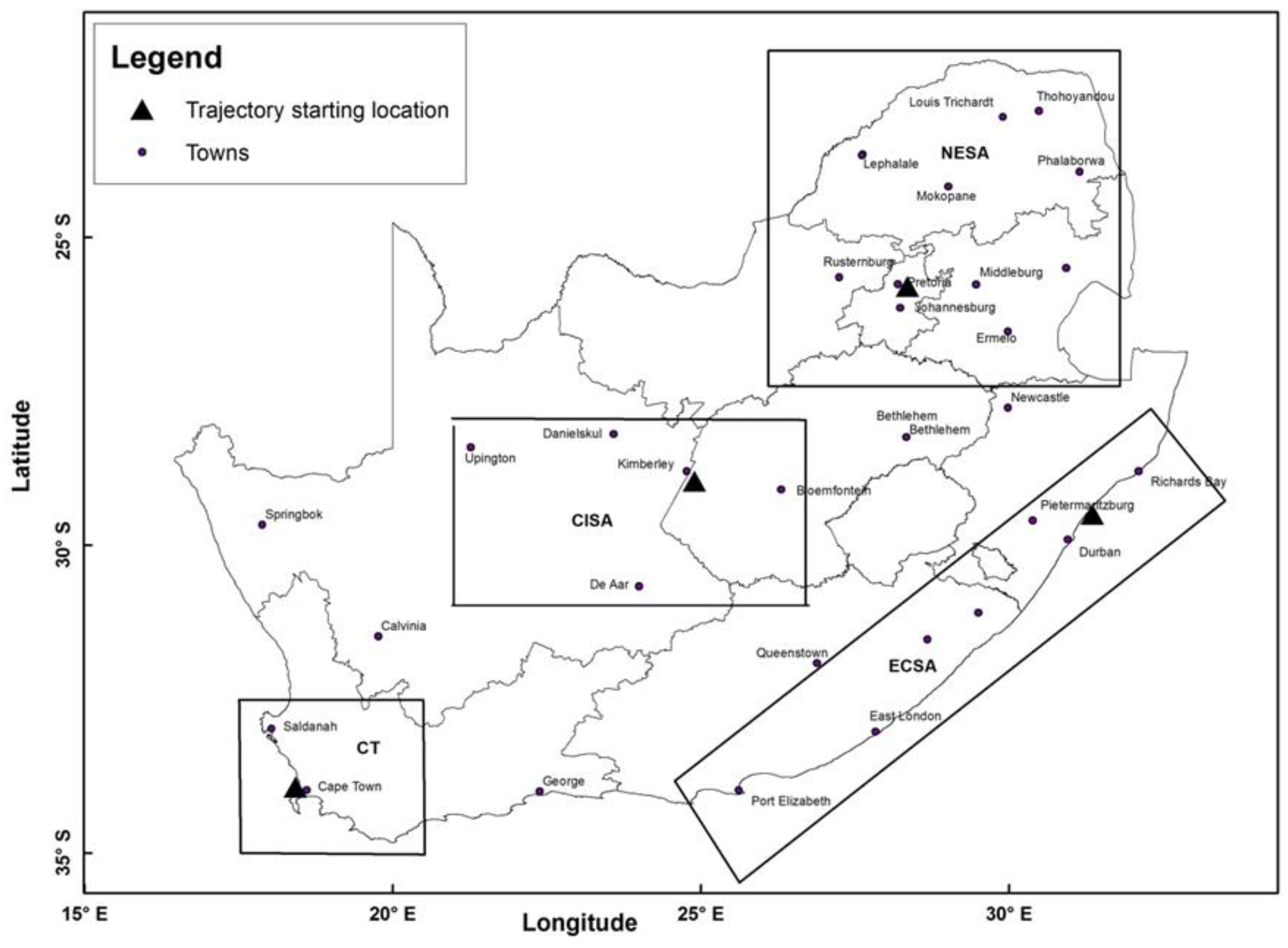
2.3. Air Transport Analysis

Hybrid Single-Particle Lagrangian Integrated Trajectories (HYSPLIT) Atmospheric Transport Model

This study investigated a 5-year seasonal climatology of air transport that impacted the mixing ratios of CO2 in South Africa. This was conducted at three layers of the troposphere, namely the surface layer (ground level to 700 hPa), the layers between 700 and 500 hPa (middle troposphere), and above 500 hPa (upper troposphere). The HYSPLIT version 4 (2017) atmospheric transport model [54,55] was used to detect the source areas of the air masses impacting at various sites of interest (listed in Table 1) in South Africa. Stein et al. [54] gave a description of the establishment, advancement, and applications of the HYSPLIT model. Backward trajectories at the three tropospheric layers were run daily from 06:00 UTC over a period of five days (120 h) for the austral summer (DJF) 2004–2009, autumn (MAM) 2005–2009, winter (JJA) 2005–2009, and spring (SON) 2005–2009 seasons. Monthly files of the reanalysis data of meteorological fields were used as input data to run the backward trajectories simulations. The reanalysis data were produced by NCEP and NCAR and made available on the NOAA website ftp://arlftp.arlhq.noaa.gov/pub/archives/reanalysis. For vertical motion, the model was set at the default option zero (0), which uses the meteorological model’s vertical velocity fields and the top of the model domain was also set at the default value 10,000 magl [55]. The five day period was selected due to previous studies on intercontinental air transport between South America and South Africa and South America and the Southwest Indian Ocean (SWIO) islands, which showed that this period is sufficient for the upper air transport from South America to South Africa and SWIO islands [30,56]. The 5-year seasonal trajectories were grouped into clusters based on their spatial closeness and each cluster was represented as a mean trajectory. The HYSPLIT model generates the trajectories and automatically assigns them to different clusters. The model also computes the fraction or percentage that each trajectory’s group or cluster makes to the total of trajectories computed for the specific period of analysis [54,55,57]. Draxler et al. [55] have provided a detailed description of the methodology of cluster generation and cluster frequency computation. The HYSPLIT model generated trajectories in each cluster were averaged and their standard deviation was computed. Since the majority of the mean trajectories or clusters were zonal and varied predominantly in latitude, the latitudinal standard deviation was computed to determine the spatial deviation from the mean transport.
The analyzed HYSPLIT data had starting locations within the South African domain, bounded by (17° to 33°) E and (22° to 35°) S. To avoid reproducing similar trajectories, the seven study areas in Table 1 and Figure 1 were grouped based on their proximity to one another. Consequently, four study areas were devised for the purpose of studying air transport impacting the South African atmosphere: (1) Cape Town (CT); (2) the Central Interior of South Africa (CISA) encompassing FS and NC; (3) the East Coast of South Africa (ECSA) containing EC and KZN; and (4) the North East of South Africa (NESA) covering IHV and L. Figure 2 shows the trajectory starting position and demarcations of study areas used for the trajectory analysis. Table 2 presents the details of the starting locations and the height above ground of the backward trajectories.

3. Results

3.1. TES and Global Atmosphere Watch (GAW) Station Comparison

A total of 57 TES profiles were recorded during the period from 23/05/2005 to 28/03/2008 within 0.5° from the Cape Point GAW ground station. However, only 32 profiles were recorded on days in which ground-based data were not contaminated by continental air mass, so the comparison was made using the 32 observations. Figure 3a,b show that there was reasonably good agreement between the surface CO2 data from TES and the ground-based GAW station. There were several instances of close comparison between the two platforms and 25% of the data from both platforms had differences that fell within 1 ppm. The best comparison of the two datasets had a difference of 0.07 ppm, and the highest difference was 4.43 ppm. The correlation between the two observations is shown in Figure 3c. The correlation coefficient R2 obtained between the TES and ground-based measurements was evaluated to be 0.547. This surface correlation value is comparable with the correlation of 0.57 at 900 hPa (corrected for errors) determined during the comparison studies of TES CO2 against aircraft (HIPPO-2) profile observations in the subtropics [39]. The reasonably good comparison between the TES and Cape Point GAW ground station CO2 data implies TES data can be used with some confidence to analyze the other regions.

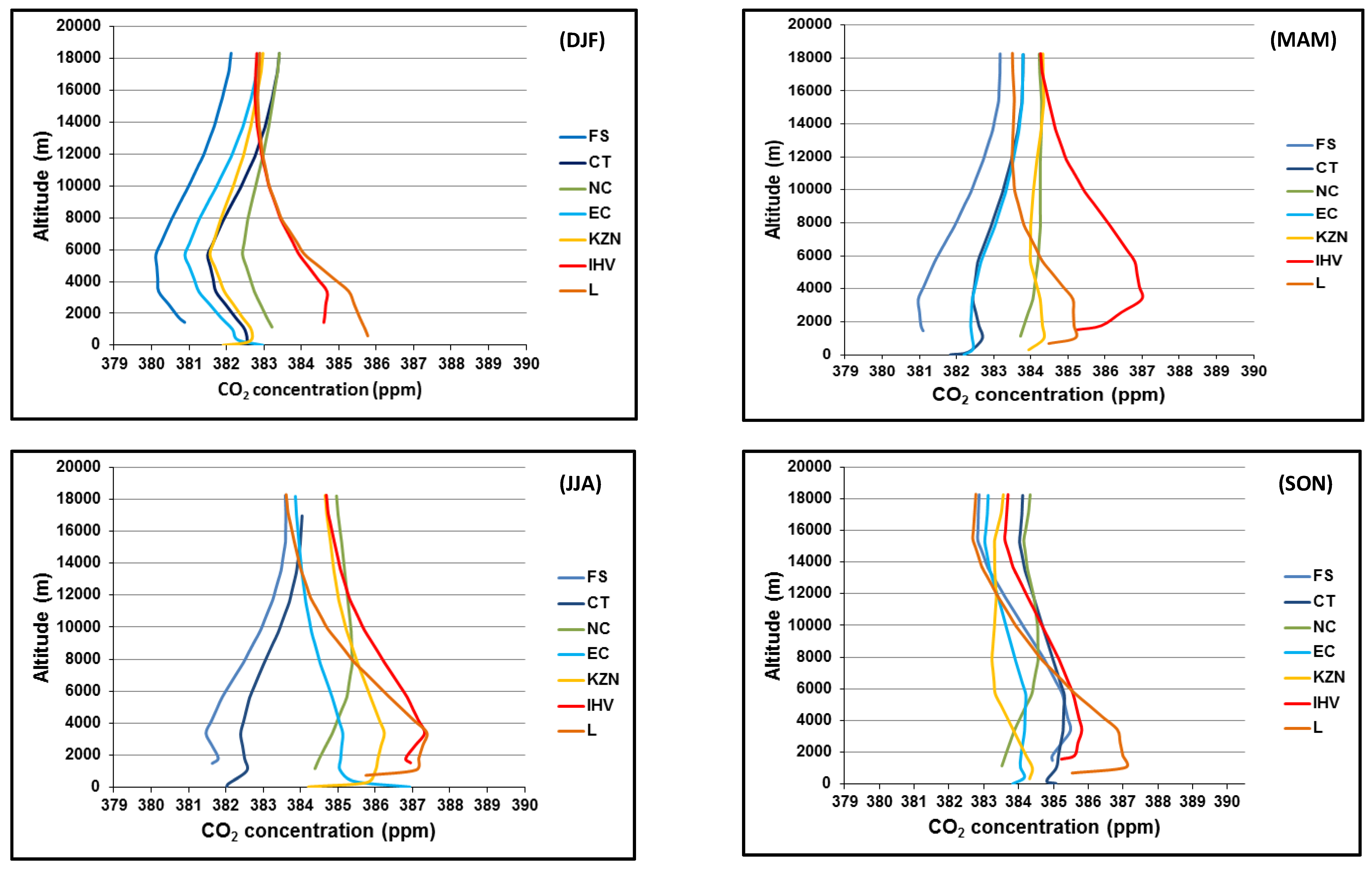
3.2. Seasonal CO2 Relative Surface Loading at the Study Areas

The seasonal loading of atmospheric CO2 at various locations in South Africa is influenced by the seasonal cycle of the strength of the emission sources. South Africa has diverse CO2 emitting sources spread out over different locations throughout the country [43,45,48,58]. In addition to the influence of local sources to the CO2 atmospheric distribution, this study also describes the dependence of the seasonal CO2 atmospheric levels on the prevailing climatological circulation patterns that influence transport and mixing [12,13,14].
Figure 4 shows the vertical distribution of CO2 in the DJF (2004–2009), MAM (2005–2009), JJA (2005–2009), and SON (2005–2009) season over the selected study areas at various locations in South Africa (Figure 1). The horizontally averaged CO2 data (used for the profiles) at different altitudes and associated standard deviations for all four seasons are provided in Table A1, Table A2, Table A3 and Table A4 in the Appendix A. Over the study period, the surface layer atmospheric loading of CO2 mostly gradually increased from the wet DJF to dry SON season (Figure 4). However, the CT area did not follow this trend, a seasonal minimum was observed during the MAM season. During the wet DJF season, the L study area had the highest averaged surface CO2 atmospheric loading, followed by the IHV, and the FS had the lowest. Over the MAM season, the IHV area had the highest averaged surface CO2 atmospheric loading followed by the L, and FS had the lowest. Similar to the DJF season, the L area had the highest averaged surface CO2 atmospheric loading followed by the IHV area, and the FS area had the lowest during the JJA season. Over the SON season, the L area had the highest averaged surface CO2 atmospheric loading followed by the IHV area, and the NC area had the lowest. The CO2 loadings are tightly connected with the emission sources within each region, thus the L and IHV areas dominated the CO2 atmospheric loading due to their relatively dense CO2 industrial sources [43] including coal-fired power generating stations [42]. The FS area had the lowest throughout the seasons due to less emissions, the exception was during the SON as it experiences biomass burning and the semiarid NC area is not [44,45]. Hence, the NC area had the lowest CO2 surface atmospheric loading during SON.

3.3. The Influence of Stable Layers in the CO2 Vertical Distribution in South Africa

During all seasons, there was a clear influence of the semi-permanent stable layers at altitudes of about 3400 m (700 hPa) and 5500 m (500 hPa) on the vertical tropospheric loading of CO2 in South Africa (Figure 4). These stable layers separated the tropospheric CO2 into three layers: (a) the surface layer, (b) the middle troposphere layer, and (c) the upper troposphere layer. However, during the JJA season, only the 700 hPa stable layer’s influence was easily notable. This could be due to the erosion of the 500 hPa stable layer as the maximum occurrence of COLs at 500 hPa is during JJA in the mid-latitude and subtropical region of the Southern Hemisphere [22]. Another observation was the discernible influence of the stable layer at an altitude of 8000 m (350 hPa) on the vertical profile of CO2 during the MAM, JJA, and SON seasons in the NC study area. This influence of the 8000 m altitude stable layer was also noticeable in the KZN study area during the SON season. The stable layers exert control on the vertical motion of air over the subcontinent by effectively inhibiting the mixing of air parcels between the different atmospheric layers [12,13,14].
The span of the average CO2 mole fractions amongst the study sites in Figure 4 varied from the ground level to the top of the troposphere in all seasons. At the ground level, it was about 5 ppm during DJF, MAM, and JJA; during SON it was about 3 ppm. At the 3400 m stable layer, it was about 5 ppm during DJF, MAM, and JJA; it narrowed to about 3 ppm during SON. At the 5500 m stable layer, it was about 4 ppm during DJF and increased to about 5 ppm during MAM and JJA, and then narrowed considerably to about 2 ppm during SON. The SON season with the highest seasonal burden of atmospheric CO2 had the most uniform distribution of CO2 on a national scale from the ground to the top of the troposphere, as the background mixing ratios shifted to higher values. This was due to the expansive spread of CO2 emissions from biomass burning, as SON is the peak season for biomass fires in Southern Africa [45]. The middle troposphere layer had the greatest span in CO2 atmospheric mixing ratio and the top of the troposphere had the least mixing ratio span of approximately 1 ppm in all seasons (Figure 4). The middle troposphere layer was decoupled from the surface and the upper troposphere layer by the 3400 and 5500 m stable layers. The standard deviations in Table A1, Table A2, Table A3 and Table A4 show that in all seasons, the spatial variability of the CO2 mixing ratio reached the maximum about the 3400 m altitude stable layer at all study sites. Above this layer, the spatial variation decreased with an increase in altitude up to the top of the troposphere. The decrease in spatial variation with an increase in altitude was clearer above the 5500 m altitude stable layer as the upper air was more uniformly mixed. The areas with relatively dense industrial CO2 sources, KZN, IHV, and L [43], had the highest surface CO2 spatial variation.

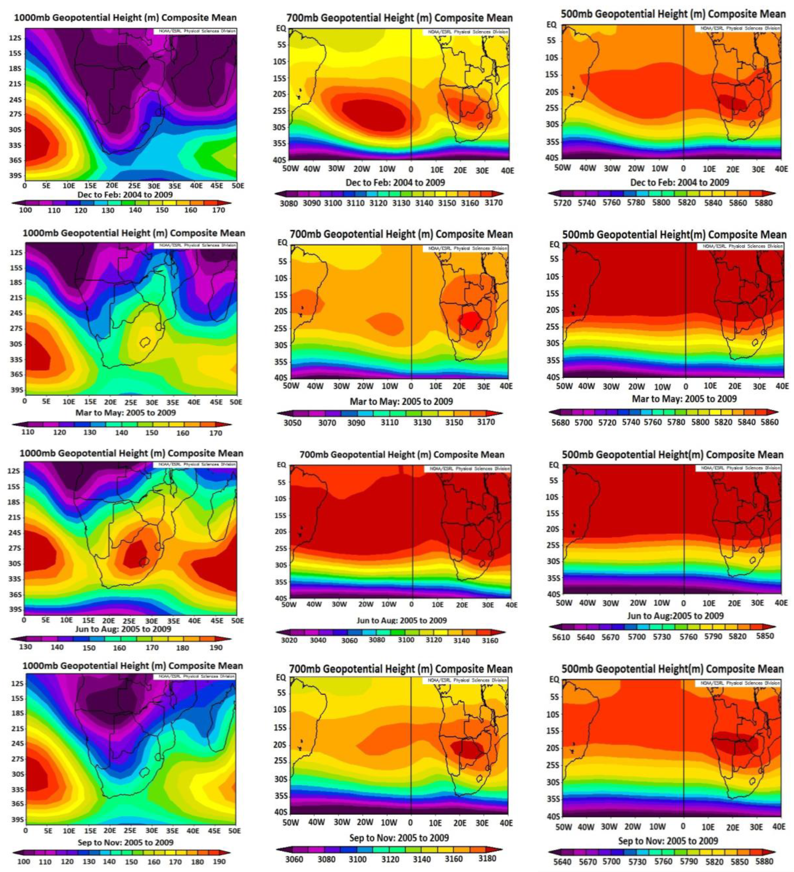
3.4. Seasonal Circulation Patterns at Different Levels of the Troposphere over Southern Africa and the South Atlantic Ocean

Figure 5 shows the mean seasonal circulation patterns over Southern Africa, the South Atlantic, and Indian Ocean at the 1000, 700, and 500 hPa pressure levels during 2004–2009. At the 1000 hPa level during DJF, the Southern Africa subcontinent was dominated by a continental trough [12,13], indicated by low geopotential height values [59] and was also flanked by anticyclone systems at the South Atlantic, and Indian Ocean [12,13], indicated by the high geopotential height values [59,60]. During MAM, this 1000 hPa level continental trough shifted northward as it was displaced by the ridging South Atlantic and Indian Ocean anticyclone. The 1000 hPa level geopotential height values in central Southern Africa reached a maximum during JJA, as the continental anticyclone is the dominant circulation system during this season [12,13,14,18]. During JJA, the low values of the 1000 hPa level geopotential height in the mid-latitudes extended northward to the southern part of the subcontinent, indicating the transient mid-latitude convective westerly wave impacts the southern parts of South Africa [47]. During SON, the 1000 hPa continental trough shifted southward to the center of the subcontinent, pushing the South Atlantic and Indian Ocean anticyclones southwest and southeast of the subcontinent, respectively. This movement is indicated by the development of low geopotential height values at the center of the subcontinent and the development of high geopotential height values southwest and southeast of the subcontinent.
The middle and right columns of Figure 5 show that Southern Africa and the South Atlantic Ocean were dominated by anticyclonic systems at 700 and 500 hPa levels, as indicated by the high geopotential height values [59,60]. Just west of the subcontinent at the 700 hPa level, the disturbance of the subtropical anticyclone system by the mid-latitude trough (low geopotential heights) was clearly discernable in all seasons and was not pronounced at the 500 hPa level. At both these pressure levels, the maximum geopotential height values (maximum anticyclone intensity) had the largest spatial extent during JJA, followed by SON.

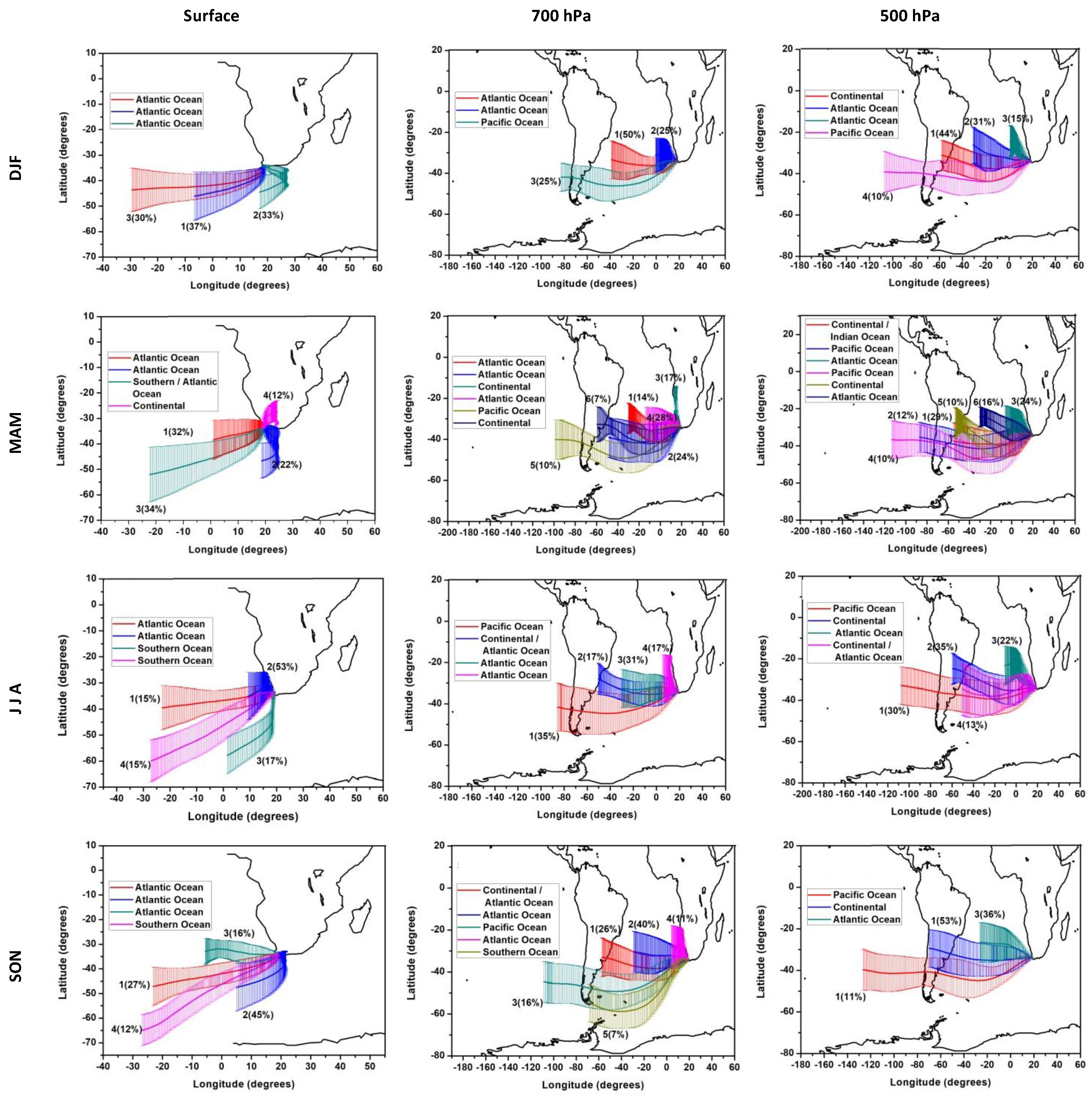
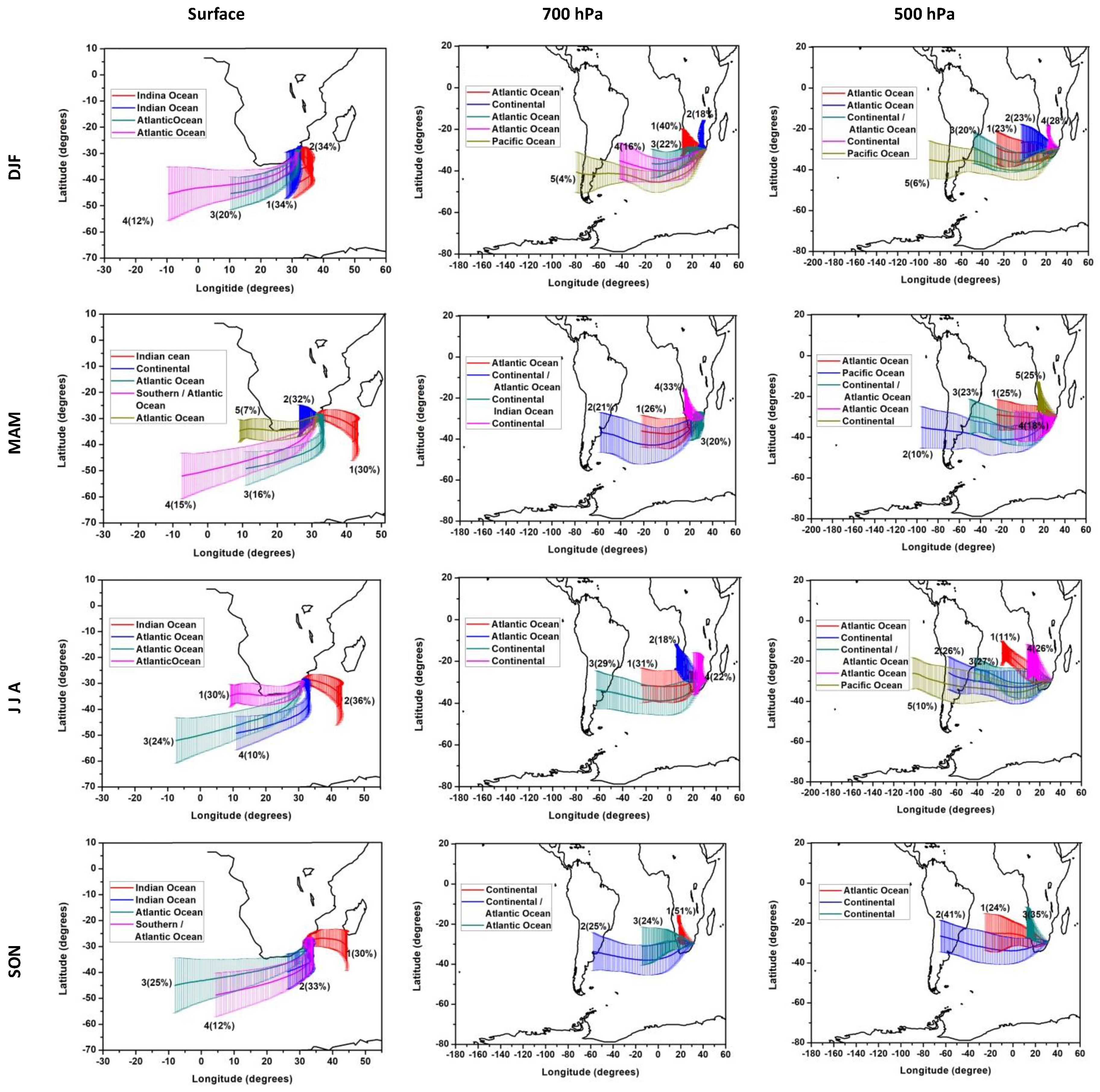
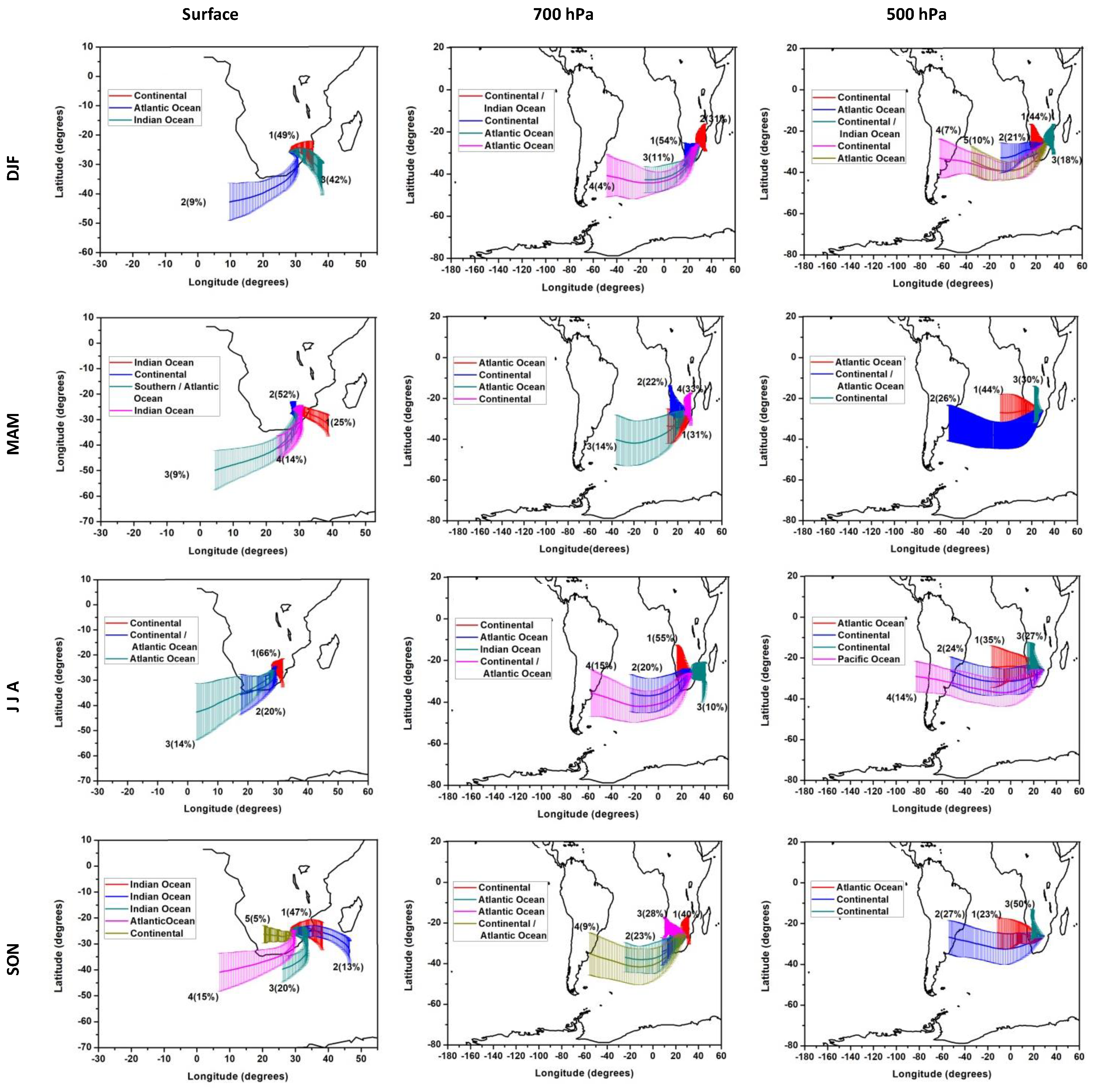
3.5. Seasonal Air Transport Backward Trajectories at Different Layers of The Troposphere in South Africa

3.5.1. Cape Town

Figure 6 presents the seasonal backward trajectories of air transport that influenced the CO2 levels at CT at the surface, above 3400, and 5500 m altitude stable layers during 2004–2009. The DJF and SON season backward surface trajectories from the CT study area were dominated by air flow from the South Atlantic Ocean that exited CT over its west coast. This transport was 100% frequent during DJF and 88% during SON. The MAM and JJA season backward surface trajectories from the CT study area were dominated by a westerly flow with frequencies of 66% and 83%, respectively. The middle and right columns of Figure 6 show that the upper air layers over the CT study area between 3400 and 5500 m, and above the 5500 m altitude were impacted by air that was from above the South Atlantic Ocean, South America, and the southeast Pacific Ocean. At 700 hPa, the transport frequency of the air from above South America increased from MAM (7%) to SON (26%) and this transport did not occur in DJF. At 500 hPa, this transport was also dominant (53%) during SON.

3.5.2. Central Interior of South Africa (CISA)

Figure 7 presents the seasonal backward trajectories of air transport that influenced the CO2 levels at the CISA study area at the surface, above 3400, and 5500 m altitude stable layers during 2004–2009. The surface of the CISA area was dominated by the transport of air from Southern Africa, with an increasing frequency from the DJF (53%) to JJA (70%) season. The influence of the westerly transport at the surface in the CISA study area increased from DJF (11%) to SON (37%). The middle and right columns of Figure 7 show that the middle and upper troposphere layers over the CISA were impacted by air that was from aloft northeast South Africa, the countries north of South Africa, and air from above the South Atlantic Ocean, South America, and southeast Pacific Ocean. The CISA area was dominated by the transport of air from above Southern Africa at the 700 hPa level in all seasons, its frequency decreased from DJF (72%) to SON (37%). At 500 hPa, this transport was limited to DJF (38%) and MAM (30%). Transport of air from above the South Atlantic Ocean was the second dominant at 700 hPa and occurred in all seasons; its frequency increased from the DJF (19%) to SON (58%) season. At 500 hPa this transport also occurred in all seasons, however with a small seasonal variation. The DJF and SON season frequencies were both 62%; the MAM season had the lowest frequency of 58%; and the JJA season had the highest frequency of 67%. The other important air transport mode that impacted the CISA area at 500 hPa was the transport of air from above South America, but was limited to JJA (27%) and SON (38%). The westerly transport of air from above the South Atlantic Ocean and South America to Southern Africa was more frequent during the dry seasons (JJA and SON).

3.5.3. East Coast of South Africa (ECSA)

Figure 8 presents the seasonal backward trajectories of air transport that influenced the CO2 levels at the ECSA study area at the surface, above 3400, and 5500 m altitude stable layers during 2004–2009. The DJF and SON season backward surface trajectories from the ECSA study area were exclusively dominated by flows from the South Indian and Atlantic Ocean. The South Indian Ocean transport was dominant in both the DJF (68%) and SON (63%) seasons and persisted across all seasons. The MAM and JJA backward surface trajectories from ECSA showed a westerly flow from the Atlantic Ocean, which was more frequent during JJA (30%). The middle and right columns of Figure 8 show that the middle and upper troposphere layers over the ECSA study area were largely impacted by air that was aloft the countries north of South Africa, the South Atlantic Ocean, and South America. The most prevalent transport that impacted the ECSA area at the 700 hPa level was the transport of air from above Southern Africa. This occurred in all seasons, with the highest frequency during DJF (58%) and the least during JJA (22%). At 500 hPa, this transport was limited to DJF (28%) and MAM (25%). The other important transport that affected the ECSA area at the 700 hPa atmospheric level was the transport of air from above South America and the South Atlantic Ocean. Both these modes of transport occurred in all seasons, excluding DJF for the South American transport, and the transport had the highest frequency of occurrence during JJA of 29% and 49%, respectively. At 500 hPa, the South Atlantic Ocean transport occurred in all seasons, with a comparable frequency for DJF (66%), MAM (66%), and JJA (64%), and its minimum frequency occurred during SON (24%). The South American transport at 500 hPa only occurred during JJA (26%) and SON (41%).

3.5.4. North East of South Africa (NESA)

Figure 9 presents the seasonal backward trajectories of air transport influencing the CO2 levels at the NESA study area at the surface, above 3400, and 5500 m altitude stable layers during 2004–2009. The NESA area was dominated by surface continental air transport from the Southern Africa subcontinent, where its frequency increased from the DJF (49%) to JJA (66%) season. The westerly air transport from the South Atlantic Ocean to the NESA was most frequent during JJA (34%). During the SON season, the on-shore surface transport from the South Indian Ocean was the most frequent (80%) transport impacting the NESA area.
The middle and upper troposphere layers over the NESA study area were mainly impacted by air originating aloft the countries north of South Africa, the South Atlantic Ocean, and South America. The NESA area was dominated by the transport of air above Southern Africa at the 700 hPa level in all seasons. The seasonal frequency of occurrence of this transport was highest during DJF (85%) and followed by SON (68%). At 500 hPa, this transport was dominant in DJF (62%) and least frequent during JJA (27%). The westerly transport of air from above the South Atlantic Ocean was the second dominant transport impacting the NESA area at the 700 hPa level and occurred in all seasons. It was most frequent (45%) in the MAM and least frequent (15%) in the DJF season. Similarly at 500 hPa, this transport was most frequent (44%) in the MAM and least frequent (31%) in the DJF season. The other important transport at 700 hPa though least frequent was transport of air from above South America, which occurred during the JJA (15%) and SON (9%) seasons. At 500 hpa, this transport occurred at all seasons and increased from the DJF (7%) to the SON (27%) season.

4. Discussion

The seasonal air transport impacting various areas in South Africa at different layers of the troposphere is influenced by the prevailing atmospheric circulation. Previous studies on circulation patterns over Southern Africa established that they have a seasonal cycle [17,18]. This section discusses the link between the seasonal meteorology and air transport established by this study; known emission sources and atmospheric distribution of CO2 over the South African atmosphere.
The DJF and SON season’s surface anticyclonic flows that impacted the CT study area (Figure 6) resulted in subsiding flows, which caused warm and dry off-shore flows over the CT west coast, creating a favorable environment for the development and spread of wildfires [61,62,63]. Natural Fynbos vegetation combustion occurs over the CT area between the warm and dry months of November to March [64]. As a consequence of this warm and dry off-shore flow driven by the South Atlantic anticyclone (Figure 5), the DJF surface CO2 loading was not the season of minimum CO2, and followed the SON CO2 loading, which was a season of maximum CO2 (Figure 4). The surface westerly flow influenced by the transient mid-latitudes westerly wave (Figure 5) dominated the CT study area during MAM and JJA, though was more prevalent during JJA than MAM (Figure 6). It brings clean maritime air from the South Atlantic and the Southern Oceans to southern parts of South Africa [47]. The consequence of the dominance of the westerly flow is the seasonal minimum in surface CO2 mixing ratio at CT in MAM (Figure 4). The higher surface CO2 mixing ratios during JJA than MAM, despite the presence of more westerly flow conditions, are a result of higher CO2 emissions from the domestic and industrial energy sector, which reached a peak during JJA in response to peak demand for energy in this season [29,48].
The CISA study area was impacted at the surface by the anticyclonic continental air transport and westerly flows from the South Atlantic Ocean in all seasons (Figure 7). The anticyclonic flow in DJF and MAM was influenced by the combination of the ridging high along the east coast and the easterly wave (Figure 5). The transport of continental air from Southern Africa was most dominant during JJA (Figure 7). The westerly transport of South Atlantic Ocean air to the CISA area was most dominant during SON. Figure 4 shows a consistent increase in surface layer CO2 from DJF to SON in the NC and FS, which are constituents of the CISA study area, with an exception at NC during SON. The seasonal shift was due to an increase in biomass burning emissions from MAM and reached its peak during SON [45]. However, Figure 4 also shows that SON was not the season of maximum surface CO2 loading at NC, as this study area is semiarid and sparsely vegetated [44,45].
The ECSA study area during DJF and SON was exclusively dominated by surface flows of marine air from the South Indian and Atlantic Ocean (Figure 8). These flows were influenced by the ridging highs (Figure 5). The ECSA study area was also impacted by the westerly flow from the Atlantic Ocean (Figure 8), which was more regular during JJA. Figure 4 shows a seasonal maximum surface layer CO2 mixing ratio during JJA at both EC and KZN. Both the EC and KZN areas are constituents of the ECSA study area. The JJA seasonal maximum at both study areas could have been influenced by the seasonal peak of the westerly flow (Figure 8), which transports emissions from the interior to their exit over the east coast [12,13,48].
Like in the CISA study area, the NESA study area was impacted at the surface by the continental air transport from the Southern Africa subcontinent and westerly flows from the South Atlantic Ocean from DJF to SON. Both the continental and westerly air transports were most frequent during the JJA season (Figure 9). Figure 4 shows that the seasonal maximum surface layer CO2 mixing ratio occurred during JJA at IHV. At L, the highest surface mixing ratio was comparable and occurred during JJA and SON. Both the IHV and L areas are constituents of NESA study area. The JJA seasonal maximum at both study areas could have been due to the energy related emissions, which are at their peak during JJA [48] including other industrial CO2 sources [43]. The transportation of biomass burning emissions laden air masses from countries north of South Africa by the surface continental flow that is prevalent during JJA also played a part in the JJA peak surface CO2 at IHV and L (Figure 9).
The seasonal climatological changes in surface atmospheric circulation patterns played an important role in the surface seasonal changes of the CO2 mixing ratios at the study areas. The dominant easterly wave in DJF (Figure 5) causes unstable atmospheric conditions over the interior that are favorable for the rapid vertical dispersion of air, mixing, deposition by rainfall [12,13,14], and carbon uptake by vegetated ecosystems through photosynthesis [11,28]. From MAM onward, the easterly wave was replaced by stability inducing anticyclones. During JJA and SON, the continental and ridging anticyclones along the east coast were prevalent (Figure 5). The anticyclones limit the vertical dispersion of air, leading to the accumulation of air pollution in a shallow mixing layer [12,13,14,48], thereby contributing to a seasonal increase in surface CO2, which reaches its peak during SON, the peak season of biomass burning in South Africa [45].
The middle and upper troposphere layers in the study areas were impacted by easterly flowing air from above the South Atlantic Ocean, South America, and the southeast Pacific Ocean; and the transport of air from above countries north of South Africa in the subcontinent. At both the middle and upper troposphere layers, the westerly air transport was dominant during JJA and SON, particularly from air above South America (Figure 6, Figure 7, Figure 8 and Figure 9). This transport was influenced by the anticyclone systems at 700 hPa and 500 hPa (Figure 5). The westerly air transport can be burdened by the biomass emissions from South America and Southern Africa (recirculated air) during JJA and SON [16,17,19] including the wide-ranging season (April to November) of sugarcane burning [25]. In these layers, elevated concentrations of vegetation combustion emissions have been observed being transported from South America to Southern Africa [17,24]. The air transport at the middle and upper troposphere from above the countries north of South Africa occurred in all seasons at the 700 hPa level at the study regions, except for CT. At 500 hPa, it occurred in the DJF and MAM seasons, except at NESA where it occurred in all seasons (Figure 6, Figure 7, Figure 8 and Figure 9). This transport was influenced by the trough systems at 700 and 500 hPa (Figure 5) as they transported the air masses in the northwest–southeast direction (Figure 6, Figure 7, Figure 8 and Figure 9). From MAM, this transport brings the biomass emissions to South Africa, as the fires start in the MAM season in northern Angola and the Southern Democratic of Congo and move southward [45,48].
Figure 4 shows that during DJF, in all the study areas with the exception of IHV and L areas, CO2 decreased less with altitudes between the 3400 and 5500 m layer than at the surface layer and then increased with altitude above 5500 m. Throughout the other seasons in the CT area, CO2 increased with altitude from just above the 3400 m stable layer all the way up to the top of the troposphere, except during SON where CO2 decreased with altitude above the 5500 m stable layer (Figure 4). The increase with the altitude of CO2 was caused by the long-range transported air masses carrying high levels of CO2 from South America (Figure 6) as the continent has a long season of biomass burning [16,17,19,25]. However during SON, the peak period for biomass burning in South Africa [45], local biomass burning emissions are strong, therefore, the free troposphere transported CO2 is relatively dilute in comparison to the surface, hence the decrease with the altitude of CO2 above the 5500 m stable layer (Figure 4).
From MAM to SON, the CO2 profiles over the NC area increased with altitude from the surface layer up to 8000 m (the level of the 350 hPa stable layer) and then decreased or showed no change with an increase in altitude (Figure 4). The increase in the slope of the CO2 profiles over the NC area from the surface layer and the layer between 3400 m and 5500 m, and the layer above 5500 m during MAM, JJA, and SON was particularly steep, which could have been due to the area being a weak emission source and the steep increase of CO2 with height to high altitudes was caused by transported air masses aloft. Figure 7 shows the frequent transport of air from above countries north of South Africa and South America in MAM and JJA at the middle and the upper troposphere layers.
During MAM and JJA, CO2 in the FS area increased with altitude from above the 3400 m altitude stable layer all the way up to the top of the troposphere (Figure 4). This was similar in NC, where air transport at these upper layers was from above strong biomass emission source regions, that is, countries north of South Africa and South America (Figure 7). During the SON season, biomass burning is at its peak in South Africa [45], hence biomass combustion emissions are strong, as a result, the free troposphere transported CO2 is relatively dilute in comparison to the surface, hence the decrease with altitude of CO2 above the 5500 m stable layer at FS (Figure 4).
During MAM, CO2 in the EC area increased with altitude from above the 3400 m altitude stable layer all the way up to the top of the troposphere (Figure 4). This could be due to the transportation of air from above countries north of South Africa (Figure 8) as biomass burning in these countries start in MAM [45,48]. During JJA, CO2 decreased with altitude from above the 3400 m altitude stable layer all the way up to the top of the troposphere (Figure 4). During SON, due to the peak incidence of biomass fires [45], the biomass combustion emissions are strong and surface emissions from various sources during JJA are also strong [48], as a result, the long-range free troposphere transported CO2 could have been relatively dilute in comparison to the surface, hence the decrease with the altitude of CO2 above the 3400 m stable layer during JJA and the 5500 m stable layer during SON (Figure 4).
Unlike the other areas during MAM, CO2 in the KZN area slightly decreased with altitude within the layer from 3400 to 5500 m and moderately increased with altitude above the 5500 m altitude stable layer all the way up to the top of the troposphere (Figure 4). The moderate increase above the 5500 m layer could be the result of the transportation of biomass emissions burdened air from above countries north of South Africa (Figure 8). Like with the case in the EC area, during JJA, CO2 in KZN decreased with altitude from above the 3400 m altitude stable layer all the way up to the top of the troposphere (Figure 4). Similar to the EC area, during SON, the peak biomass fires emissions [45], and surface emissions from various sources during JJA are also strong [48]. As a result, CO2 from the long-range free troposphere transport (Figure 8) could have been relatively dilute in comparison to the surface, hence the decrease with altitude of CO2 above the 3400 m stable layer during JJA (Figure 4) and lower CO2 mixing ratio levels above 5500 m during SON (Figure 4).
Figure 4 shows that in the IHV and L areas in all seasons, CO2 decreased with altitude from just above the 3400 m altitude stable layer all the way up to the top of the troposphere. This is due to the fact that both areas have a high concentration of industrial CO2 sources including coal-based power generation stations [42,43], some having slight seasonal emission strength cycle [47]. The seasonal biomass and domestic fossil fuel burning emissions are also important contributors to CO2 emissions in these areas [11,45,48]. Consequently, the free troposphere transported CO2 (Figure 9) is relatively dilute in comparison to the surface CO2, hence the decrease with altitude of CO2 just above the 3400 m stable layer in all seasons (Figure 4).

5. Conclusions

This study demonstrated that the relative atmospheric loading of CO2 at various regions in South Africa is intimately linked with emission sources within each region. However, meteorology and air transport also play an important role in influencing the atmospheric mixing ratio distribution of CO2 in South Africa at different atmospheric levels. The subtropical semi-permanent stable layers over South Africa separate the tropospheric CO2 into layers of different loading. Meteorology and air transport lead to the accumulation or dilution of atmospheric levels of CO2 at various sites in South Africa where this change is dependent on the transport source region and type of air flow. The long-range air transport from different source regions at the upper air level between the 700 and 500 hPa stable layers and the layer above 500 hPa strengthens the inhomogeneity in the vertical distribution of CO2, which is caused by the decoupling effect of the upper air stable layers. At some areas in South Africa, this free troposphere long-range air transport can result in higher free troposphere CO2 mixing ratios than the CO2 mixing ratios at the surface. The middle and upper troposphere westerly long-range air transport also involves intercontinental air transport, which is more frequent during winter and spring.

Author Contributions

Conceptualization, X.G.N.; Methodology, X.G.N. and V.S.; Formal Analysis, X.G.N.; Investigation, X.G.N.; Writing—Original Draft preparation, X.G.N.; Writing—Review & Editing, X.G.N., V.S., and O.E.M.; Supervision, V.S. All authors have read and agreed to the published version of the manuscript.

Funding

This research received no external funding.

Acknowledgments

We would like to thank the University of KwaZulu-Natal School of Chemistry and Physics, Bureau Océan Indien of the Agence Universitaire de la Francophonie (AUF) for supporting the study. We gratefully acknowledge the NASA Langley Research Center for making the TES/Aura CO2 data available online. The South African Weather Service’s Global Atmosphere Watch station personnel are gratefully acknowledged for providing the ground-based CO2 data. We thank NOAA ARL for providing the reanalysis data to compute the backward trajectories using the HYSPLIT model, which were used in this publication. We gratefully acknowledge NCEP, NCAR, and NOAA/ESRL: PSD for providing the reanalysis data and plots. We would also like to thank Lee-ann Simpson for proofreading the document.

Conflicts of Interest

The authors declare that they have no conflicts of interest.

Appendix A

Table A1. Summer (DJF) horizontally averaged CO2 data and the associated standard deviations at different altitudes used for vertical profiles at different study areas.
Altitude (m)CTCTNCECKZNIHVL
CO2 ± STD (ppm)CO2 ± STD (ppm)CO2 ± STD (ppm)CO2 ± STD (ppm)CO2 ± STD (ppm)CO2 ± STD (ppm)CO2 ± STD (ppm)
0.02 382.22 ± 6 382.97 ± 6381.91 ± 6
230.64 382.53 ± 6 382.30 ± 6382.60 ± 6
592.67 385.77 ± 12
942.04 382.49 ± 6383.21 ± 10382.16 ± 5382.67 ± 7 385.71 ± 10
1440.94380.88 ± 7 384.60 ± 9
1756.64380.73 ± 7382.23 ± 6383.08 ± 11381.85 ± 6382.42 ± 7384.62 ± 9385.55 ± 10
2569.40380.46 ± 8381.97 ± 7382.91 ± 11381.56 ± 6382.18 ± 8384.65 ± 10385.41 ± 11
3370.16380.19 ± 9381.72 ± 7382.74 ± 12381.27 ± 6381.94 ± 9384.68 ± 10385.27 ± 11
4156.60380.16 ± 8381.64 ± 7382.64 ± 11381.14 ± 6381.81 ± 9384.43 ± 10384.87 ± 10
4929.14380.14 ± 8381.57 ± 7382.53 ± 10381.01 ± 6381.69 ± 9384.19 ± 9384.47 ± 9
5688.85380.12 ± 8381.50 ± 7382.43 ± 9380.89 ± 6381.56 ± 8383.94 ± 9384.08 ± 8
6435.90380.25 ± 7381.64 ± 7382.47 ± 8381.01 ± 6381.65 ± 8383.77 ± 8383.88 ± 8
7169.57380.39 ± 7381.77 ± 6382.52 ± 8381.13 ± 5381.75 ± 8383.61 ± 8383.67 ± 7
7889.28380.53 ± 6381.91 ± 6382.57 ± 7381.26 ± 5381.84 ± 7383.45 ± 7383.47 ± 6
8594.71380.68 ± 6382.06 ± 6382.63 ± 6381.41 ± 5381.95 ± 7383.34 ± 6383.36 ± 6
9286.01380.83 ± 5382.22 ± 5382.70 ± 6381.56 ± 4382.06 ± 6383.24 ± 6383.25 ± 5
10627.13381.12 ± 4382.50 ± 4382.84 ± 5381.85 ± 4382.27 ± 5383.07 ± 5383.08 ± 4
13151.47381.58 ± 3382.93 ± 4383.08 ± 4382.33 ± 3382.58 ± 4382.86 ± 4382.90 ± 3
14343.87381.75 ± 3383.09 ± 3383.17 ± 3382.51 ± 3382.70 ± 4382.80 ± 4382.86 ± 3
15502.97381.89 ± 3383.21 ± 3383.25 ± 3382.65 ± 3382.79 ± 3382.76 ± 4382.83 ± 3
17761.56382.09 ± 3383.39 ± 3383.39 ± 3382.84 ± 3382.95 ± 3382.80 ± 3382.88 ± 3
18325.96382.12 ± 3383.41 ± 3383.41 ± 3382.87 ± 3382.97 ± 3382.81 ± 3382.89 ± 3
Table A2. Autumn (MAM) horizontally averaged CO2 data and the associated standard deviations at different altitudes used for vertical profiles at the different study areas.
Altitude (m)FSCTNCECKZNIHVL
CO2 ± STD (ppm)CO2 ± STD (ppm)CO2 ± STD (ppm)CO2 ± STD (ppm)CO2 ± STD (ppm)CO2 ± STD (ppm)CO2 ± STD (ppm)
4.07 381.84 ± 7 382.20 ± 7381.36 ± 6
345.94 382.32 ± 7 382.44 ± 7383.94 ± 7
686.11 384.48 ± 9
1054.03 382.70 ± 7.1383.72 ± 6382.42 ± 7384.34 ± 8 385.19 ± 10
1440.94381.10 ± 7 385.24 ± 6
1766.61381.04 ± 7382.60 ± 7383.81 ± 6382.38 ± 7384.31 ± 8385.90 ± 7385.16 ± 10
2566.75381.00 ± 7382.52 ± 8383.93 ± 6382.40 ± 8384.28 ± 8386.44 ± 8385.15 ± 10
3353.82380.97 ± 7382.44 ± 8384.05 ± 7382.42 ± 8384.25 ± 9386.98 ± 8385.13 ± 10
4126.94381.12 ± 7382.48 ± 8384.10 ± 6382.50 ± 8384.16 ± 8386.92 ± 8384.85 ± 10
4886.25381.26 ± 6382.52 ± 8384.15 ± 6382.58 ± 8384.08 ± 8386.86 ± 8384.58 ± 9
5631.52381.41 ± 6382.57 ± 7384.19 ± 6382.66 ± 7383.99 ± 8386.80 ± 8384.31 ± 8
6362.36381.59 ± 6382.69 ± 7384.21 ± 6382.78 ± 7383.99 ± 7386.57 ± 7384.14 ± 8
7078.55381.77 ± 5382.80 ± 6384.24 ± 5382.90 ± 6383.99 ± 6386.35 ± 7383.98 ± 7
7780.00381.95 ± 5382.92 ± 6384.26 ± 5383.03 ± 6384.00 ± 6386.13 ± 6383.81 ± 6
8466.52382.09 ± 5383.02 ± 5384.26 ± 5383.12 ± 5384.02 ± 5385.90 ± 6383.73 ± 6
9138.38382.24 ± 4383.13 ± 5384.26 ± 4383.22 ± 5384.04 ± 5385.68 ± 5383.65 ± 5
10440.52382.49 ± 4383.31 ± 4384.26 ± 4383.38 ± 4384.10 ± 4385.29 ± 5383.54 ± 4
12915.24382.89 ± 3383.58 ± 3384.27 ± 3383.62 ± 3384.24 ± 3384.76 ± 4383.52 ± 3
14115.41383.02 ± 3383.68 ± 3384.29 ± 3383.70 ± 3384.30 ± 3384.60 ± 3383.54 ± 3
16470.88383.16 ± 3383.78 ± 3384.26 ± 3383.78 ± 3384.34 ± 3384.36 ± 3383.53 ± 3
17636.66383.17 ± 3383.79 ± 3384.23 ± 3383.79 ± 3384.33 ± 3384.28 ± 3383.51 ± 3
Table A3. Winter (JJA) horizontally averaged CO2 data and the associated standard deviations at different altitudes used for vertical profiles at the different study areas.
Altitude (m)FSCTNCECKZNIHVL
CO2 ± STD (ppm)CO2 ± STD (ppm)CO2 ± STD (ppm)CO2 ± STD (ppm)CO2 ± STD (ppm)CO2 ± STD (ppm)CO2 ± STD (ppm)
6.05 382.02 ± 6 386.92 ± 7384.21 ± 8
363.48 382.06 ± 6 385.42 ± 6385.77 ± 8
718.73 385.75 ± 8
1047.34 382.56 ± 7384.39 ± 5385.06 ± 7386.00 ± 8 387.09 ± 10
1466.64381.63 ± 6 386.94 ± 10
1769.49381.79 ± 7382.50 ± 7384.50 ± 5385.07 ± 7386.07 ± 9386.82 ± 10387.17 ± 10
2558.37381.63 ± 7382.45 ± 7384.67 ± 5385.10 ± 7386.16 ± 9387.07 ± 11387.27 ± 10
3334.02381.47 ± 7382.40 ± 8384.85 ± 5385.13 ± 7386.24 ± 9387.32 ± 12387.38 ± 11
4096.52381.61 ± 7382.47 ± 7384.98 ± 5385.04 ± 7386.12 ± 9387.16 ± 11387.04 ± 10
4845.48381.76 ± 7382.55 ± 7385.11 ± 5384.94 ± 6385.99 ± 8387.00 ± 10386.69 ± 9
5580.40381.90 ± 6382.63 ± 7385.24 ± 5384.85 ± 6385.87 ± 8386.85 ± 10386.35 ± 9
6300.86382.09 ± 6382.76 ± 6385.29 ± 5384.74 ± 6385.75 ± 7386.64 ± 9386.04 ± 8
7006.59382.28 ± 5382.88 ± 6385.34 ± 4384.64 ± 5385.64 ± 7386.44 ± 8385.73 ± 7
7697.68382.47 ± 5383.01 ± 6385.39 ± 4384.53 ± 5385.52 ± 6386.24 ± 8385.42 ± 6
8374.24382.62 ± 5383.14 ± 5385.37 ± 4384.45 ± 4385.42 ± 6386.06 ± 7385.19 ± 6
9037.19382.77 ± 4383.27 ± 5385.36 ± 4384.37 ± 4385.33 ± 5385.88 ± 6384.95 ± 5
9687.95382.92 ± 4383.40 ± 5385.35 ± 4384.29 ± 4385.23 ± 5385.70 ± 6384.72 ± 5
10959.93383.14 ± 4383.60 ± 4385.29 ± 3384.19 ± 3385.09 ± 4385.44 ± 5384.42 ± 4
13431.73383.48 ± 3383.88 ± 4385.18 ± 3384.03 ± 3384.89 ± 3385.07 ± 4384.00 ± 3
14642.96383.56 ± 3383.95 ± 3385.13 ± 3383.98 ± 3384.83 ± 3384.95 ± 4383.88 ± 3
17021.94383.61 ± 3384.04 ± 3385.00 ± 3383.89 ± 3384.70 ± 3384.74 ± 3383.66 ± 3
18203.22383.59 ± 3384.04 ± 3384.96 ± 3383.86 ± 3384.66 ± 3384.69 ± 3383.61 ± 3
Table A4. Spring (SON) horizontally averaged CO2 data and the associated standard deviations at different altitudes used for vertical profiles at the different study areas.
Altitude (m)FSCTNCETKZNIHVL
CO2 ± STD (ppm)CO2 ± STD (ppm)CO2 ± STD (ppm)CO2 ± STD (ppm)CO2 ± STD (ppm)CO2 ± STD (ppm)CO2 ± STD (ppm)
0.00 385.07 ± 7 383.83 ± 7382.39 ± 7
390.75 384.81 ± 7 384.16 ± 6384.31 ± 7
659.73 385.54 ± 8
1034.78 385.08 ± 7383.52 ± 6384.05 ± 6384.40 ± 8 387.07 ± 9
1461.77384.97 ± 7 385.23 ± 7
1751.32384.97 ± 7385.14 ± 7383.62 ± 6384.06 ± 6384.21 ± 8385.61 ± 7386.99 ± 10
2545.65385.24 ± 7385.21 ± 7383.74 ± 6384.12 ± 6384.03 ± 9385.70 ± 7386.92 ± 10
3327.95385.49 ± 7385.28 ± 7383.88 ± 7384.17 ± 7383.85 ± 10385.81 ± 8386.84 ± 10
4097.57385.41 ± 7385.29 ± 7384.04 ± 6384.18 ± 6383.67 ± 10385.73 ± 8386.43 ± 10
4853.96385.33 ± 7385.30 ± 7384.21 ± 6384.19 ± 6383.50 ± 11385.65 ± 8386.02 ± 9
5596.94385.26 ± 7385.31 ± 7384.37 ± 6384.21 ± 6383.33 ± 11385.56 ± 7385.61 ± 9
6326.20385.08 ± 6385.21 ± 6384.43 ± 5384.11 ± 6383.30 ± 10385.43 ± 7385.29 ± 8
7041.49384.91 ± 6385.11 ± 6384.50 ± 5384.01 ± 5383.26 ± 10385.29 ± 7384.96 ± 7
7742.91384.74 ± 6385.01 ± 6384.56 ± 5383.92 ± 5383.23 ± 9385.16 ± 6384.64 ± 7
8430.33384.55 ± 5384.91 ± 5384.55 ± 4383.83 ± 5383.25 ± 8385.00 ± 6384.40 ± 6
9104.01384.35 ± 5384.81 ± 5384.55 ± 4383.74 ± 4383.28 ± 8384.84 ± 5384.16 ± 6
9764.40384.15 ± 5384.72 ± 4384.55 ± 4383.66 ± 4383.30 ± 7384.69 ± 5383.92 ± 5
11049.05383.79 ± 4384.54 ± 4384.48 ± 3383.50 ± 4383.34 ± 6384.39 ± 4383.57 ± 4
13510.78383.12 ± 4384.18 ± 3384.25 ± 3383.17 ± 3383.31 ± 4383.84 ± 3382.94 ± 3
14707.10382.92 ± 3384.08 ± 3384.18 ± 3383.07 ± 3383.31 ± 4383.68 ± 3382.77 ± 3
17060.89382.84 ± 3384.09 ± 3384.28 ± 3383.10 ± 3383.50 ± 3383.66 ± 3382.74 ± 3
18235.79382.86 ± 3384.12 ± 3384.33 ± 3383.12 ± 3383.56 ± 3383.69 ± 3382.77 ± 3

References

  1. Intergovernmental Panel on Climate Change, Report. In Climate Change 1995. The Science of Climate Change, Contribution of Working Group I to the Second Assessment Report of the Intergovernmental Panel on Climate Change (IPCC); Cambridge University Press: Cambridge, UK; New York, NY, USA, 1996.
  2. Diallo, M.; Legras, B.; Ray, E.; Engel, A.; Añel, J.A. Global distribution of CO2 in the upper troposphere and stratosphere. Atmos. Chem. Phys. 2017, 17, 3861–3878. [Google Scholar] [CrossRef] [Green Version]
  3. Forster, P.; Ramaswamy, V.; Artaxo, P.; Berntsen, T.; Betts, R.; Fahey, D.W.; Haywood, J.; Lean, J.; Lowe, D.C.; Myhre, G.; et al. Changes in Atmospheric Constituents and in Radiative Forcing. In Change 2007: The Physical Science Basis. Contribution of Working Group I to the Fourth Assessment Report of the Intergovernmental Panel on Climate Change; Solomon, S.D., Qin, M., Manning, Z., Chen, M., Marquis, K.B., Averyt Tignor, M., Miller, H.L., Eds.; Cambridge University Press: Cambridge, UK; New York, NY, USA, 2007. [Google Scholar]
  4. World Meteorological Organization, The State of Greenhouse Gases in the Atmosphere Using Global Observations through 2013. WMO GHG Bullet. 2014, 10, 1–8, ISSN 2078-0796. Available online: https://library.wmo.int/pmb_ged/ghg-bulletin_10_en.pdf (accessed on 28 March 2019).
  5. Denman, K.L.; Brasseur, G.; Chidthaisong, A.; Ciais, P.; Cox, P.M.; Dickinson, R.E.; Hauglustaine, D.; Heinze, C.; Holland, E.; Jacob, D.; et al. Couplings Between Changes in the Climate System and Biogeochemistry. In Climate Change 2007: The Physical Science Basis. Contribution of Working Group I to the Fourth Assessment Report of the Intergovernmental Panel on Climate Change; Solomon, S., Qin, D., Manning, M., Chen, Z., Marquis, M., Averyt, K.B., Tignor, M., Miller, H.L., Eds.; Cambridge University Press: Cambridge, UK; New York, NY, USA, 2007. [Google Scholar]
  6. Deutscher, N.M.; Sherlock, V.; Mikaloff Fletcher, S.E.; Griffith, D.W.T.; Notholt, J.; Macatangay, R.; Connor, B.J.; Robinson, J.; Shiona, H.; Velazco, V.A.; et al. Drivers of column-average CO2 variability at Southern Hemispheric Total Carbon Column Observing Network sites. Atmos. Chem. Phys. 2014, 14, 9883–9901. [Google Scholar] [CrossRef] [Green Version]
  7. World Meteorological Organization, The State of Greenhouse Gases in the Atmosphere Based on Global Observations through 2011. WMO GHG Bullet. 2012, 8, 1–4, ISSN 2078-0796. Available online: https://library.wmo.int/pmb_ged/ghg-bulletin_8_en.pdf (accessed on 28 March 2019).
  8. World Meteorological Organization. The State of Greenhouse Gases in the Atmosphere Using Global Observations through 2012. WMO GHG Bullet. 2013, 9, 1–4, ISSN 2078-0796. Available online: https://library.wmo.int/pmb_ged/ghg-bulletin_9_en.pdf (accessed on 28 March 2019).
  9. World Meteorological Organization. The State of Greenhouse Gases in the Atmosphere Based on Global Observations through 2017. WMO GHG Bullet. 2018, 14, 1–8, ISSN 2078-0796. Available online: https://library.wmo.int/index.php?lvl=notice_display&id=20697#.XYtnrmZS_IV (accessed on 25 September 2019).
  10. Fang, S.X.; Zhou, L.X.; Tans, P.P.; Ciais, P.; Steinbacher, M.; Xu, L.; Luan, T. In situ measurement of atmospheric CO2 at the four WMO/GAW stations in China. Atmos. Chem. Phys. 2014, 14, 2541–2554. [Google Scholar] [CrossRef] [Green Version]
  11. Sabine, C.L.; Feely, R.A.; Gruber, N.; Key, R.M.; Lee, K.; Bullister, J.L.; Wanninkhof, R.; Wong, C.S.; Wallace, W.W.R.; Tilbrook, B.; et al. The Oceanic Sink for Anthropogenic CO2. Science 2004, 305, 367–371. [Google Scholar] [CrossRef] [Green Version]
  12. Tyson, P.D.; Garstang, M.; Swap, R.; Kållberg, P.; Edwards, M. An air transport climatology for subtropical southern Africa. Int. J. Climatol. 1996, 16, 265–291. [Google Scholar] [CrossRef]
  13. Garstang, M.; Tyson, P.D.; Swap, R.; Edwards, M.; Kållberg, P.; Lindesay, J. A Horizontal and vertical transport of air over southern Africa. J. Geophys. Res. 1996, 101, 23721–23736. [Google Scholar] [CrossRef]
  14. Swap, R.J.; Tyson, P.D. Stable discontinuities as determinants of the vertical distribution of aerosols and trace gases in the atmosphere. SAJS 1999, 95, 63–70. [Google Scholar]
  15. Moxim, W.J.; Levy II, H. A model analysis of the tropical South Atlantic Ocean tropospheric ozone maximum: The interaction of transport and chemistry. J. Geophys. Res. 2000, 105, 17393–17415. [Google Scholar] [CrossRef]
  16. Freitas, S.A.; Longo, K.M.; Silva Dias, M.A.F.; Silva Dias, P.L.; Chatfield, R.; Prins, E.; Artaxo, P.; Grell, G.A.; Recuero, F.S. Monitoring the transport of biomass burning emissions in South America. Environ. Fluid Mech. 2005, 5, 135–167. [Google Scholar] [CrossRef]
  17. Edwards, D.P.; Emmons, L.K.; Gille, J.C.; Chu, A.; Attié, J.L.; Giglio, L.; Wood, S.W.; Haywood, J.; Deeter, M.N.; Massie, S.T.; et al. Satellite-observed pollution from Southern Hemisphere biomass burning. J. Geophys. Res. 2006, 111, 14. [Google Scholar] [CrossRef]
  18. Freiman, M.T.; Tyson, P.D. The thermodynamic structure of the atmosphere over South Africa: Implications for water vapour transport. Water SA 2000, 26, 153–158. [Google Scholar]
  19. Krishnamurti, T.N.; Fuelberg, H.E.; Sinha, M.C.; Oosterhof, D.; Bensman, E.L.; Kumar, V.B. The Meteorological Environment of the Tropospheric Ozone Maximum Over the Tropical South Atlantic Ocean. J. Geophys. Res. 1993, 98, 10692–10694. [Google Scholar] [CrossRef]
  20. Romatschke, U.; Houze, R.A., Jr. Extreme Summer Convection in South America. J. Clim. 2010, 23, 3761–3791. [Google Scholar] [CrossRef]
  21. Añel, J.A.; Antuña, J.C.; de la Torre, L.; Castanheira, J.M.; Gimeno, L. Climatological features of global multiple tropopause events. J. Geophys. Res. 2008, 113, D00B08. [Google Scholar] [CrossRef] [Green Version]
  22. Reboita, M.S.; Nieto, R.; Gimeno, L.; Rocha, R.P.; Ambrizzi, T.; Garreaud, R.; Krüger, L.F. Climatological features of cuttoff low systems in the Southern Hemisphere. J. Geophys. Res. 2010, 115, D17104. [Google Scholar] [CrossRef] [Green Version]
  23. McNider, R.T.; Norris, W.B.; Song, A.J.; Clymer, R.L.; Gupta, S.; Banta, R.M.; Zamora, R.J.; White, A.B.; Trainer, M. Meteorological conditions during the 1995 Southern Oxidants Study Nashville/Middle Tennessee Field Intensive. J. Geophys. Res. 1998, 103, 22225–22243. [Google Scholar] [CrossRef]
  24. Gloudemans, A.M.S.; Krol, M.C.; Meirink, J.F.; de Laat, A.T.J.; van der Werf, G.R.; Schrijver, H.; van den Broek, M.M.P.; Aben, I. Evidence for long-range transport of carbon monoxide in the Southern Hemisphere from SCIAMACHY observations. Geophys. Res. Lett. 2006, 33. [Google Scholar] [CrossRef] [Green Version]
  25. Franca, D.; Longo, K.; Rudorff, B.; Aguiar, D.; Freitas, S.; Stockler, R.; Pereira, G. Pre-harvest sugarcane burning emission inventories based on remote sensing data in the state of São Paulo Brazil. Atmos. Environ. 2014, 99, 446–456. [Google Scholar] [CrossRef]
  26. Marenco, F.; Johnson, B.; Langridge, J.M.; Mulcahy, A.; Benedetti, A.; Remy, S.; Jones, L.; Szpek, K.; Haywood, J.; Longo, K.; et al. On the vertical distribution of smoke in the Amazon atmosphere during the dry season. Atmos. Chem. Phys. 2016, 16, 2155–2174. [Google Scholar]
  27. Williams, C.A.; Hanan, N.P.; Neff, J.C.; Scholes, J.R.; Berry, J.A.; Denning, A.S.; Baker, D.F. Africa and the global carbon cycle. Carbon Balance Manag. 2007, 2, 1–13. [Google Scholar] [CrossRef] [PubMed] [Green Version]
  28. Valentini, R.; Arneth, A.; Bombelli, A.; Castaldi, S.; Cazzolla Gatti, R.; Chevallier, F.; Ciais, P.; Grieco, E.; Hartmann, J.; Henry, M.; et al. A full greenhouse gases budget of Africa: Synthesis, uncertainties, and vulnerabilities. Biogeosciences 2014, 11, 381–407. [Google Scholar] [CrossRef] [Green Version]
  29. Nickless, A.; Ziehn, T.; Rayner, P.J.; Scholes, R.J.; Engelbrecht, F. Greenhouse gas network design using backward Lagrangian particle dispersion model—Part 2: Sensitivity analyses and South African test case. Atmos. Chem. Phys. 2015, 15, 2051–2069. [Google Scholar] [CrossRef] [Green Version]
  30. Ncipha, X.; Sivakumar, V. Influence of meteorology on carbon dioxide atmospheric loading in South Africa. In Proceedings of the V Congreso Colombiano y Conferencia Internacional de Calidad del Airey y Salud Pública, 5th Colombian Congress and International Conference of Air Quality and Public Health, Bucaramanga, Agosta, Colombia, 10–14 August 2015; Universidad de los Andes: Bogotá, Colombia, 2016; pp. 97–106. Available online: http://casap.com.co/2015/es/memorias/libro_memorias.pdf?v=2 (accessed on 1 June 2019).
  31. Schoeberl, M.R.; Douglass, A.R.; Hilsenrath, E.; Bhartia, P.K.; Waters, J.W.; Gunson, M.R.; Froidevaux, L.; Gille, J.C.; Barnett, J.J.; Levelt, P.F.; et al. Overview of the EOS Aura Mission. IEEE Trans. Geosci Remote Sens. 2006, 44, 1066–1074. [Google Scholar] [CrossRef] [Green Version]
  32. Beer, R.; Glavich, T.A.; Rider, D.M. Tropospheric emission spectrometer for the Earth Observing System’s Aura satellite. Appl Opt. 2001, 40, 2358–2367. [Google Scholar] [CrossRef]
  33. Jones, D.B.A.; Bowman, K.W.; Palmer, P.I.; Worden, J.R.; Jacob, D.J.; Hoffman, R.N.; Bey, I.; Yantosca, R.M. Potential of observations from the Tropospheric Emission Spectrometer to constrain continental sources of carbon monoxide. J. Geophys. Res. 2003, 108, D24. [Google Scholar] [CrossRef]
  34. Worden, J.; Kulawik, S.S.; Shephard, M.W.; Clough, S.A.; Worden, H.; Bowman, K.; Goldman, A. Predicted errors of tropospheric emission spectrometer nadir retrievals from spectral window selection. J. Geophys. Res. 2004, 109, D09308. [Google Scholar] [CrossRef] [Green Version]
  35. Beer, R. TES on the Aura Mission: Scientific Objectives, Measurements, and Analysis Overview. IEEE Trans. Geosci Remote Sens. 2006, 44, 1102–1105. [Google Scholar] [CrossRef]
  36. Rinsland, C.P.; Luo, M.; Logan, J.A.; Beer, R.; Worden, H.; Kulawik, S.S.; Rider, D.; Osternman, G.; Gunson, M.; Eldering, A.; et al. Nadir measurements of carbon monoxide distribution by the Tropospheric Emission Spectrometer instrument onboard the Aura Spacecraft: Overview of analysis approach and examples of initial results. Geophys. Res. Lett. 2006, 33, L22806. [Google Scholar] [CrossRef] [Green Version]
  37. Jones, D.B.A.; Bowman, K.W.; Logan, J.A.; Heald, C.L.; Liu, J.; Lou, M.; Worden, J.; Drummond, J. The zonal structure of tropical O3 and CO as observed by the Tropospheric Emission Spectrometer in November 2004-Part 1: Inverse modelling of CO emissions. Atmos. Chem. Phys. 2009, 9, 3547–3562. [Google Scholar] [CrossRef] [Green Version]
  38. Kuai, L.; Worden, J.; Kulawik, S.; Bowman, K.; Lee, M.; Biraud, S.C.; Abshire, J.B.; Wofsy, S.C.; Natraj, V.; Frakenberg, C.; et al. Profiling Tropospheric CO2 using Aura TES and TCOON instruments. Atmos. Meas. Tech. 2013, 6, 63–79. [Google Scholar] [CrossRef] [Green Version]
  39. Kulawik, S.S.; Worden, J.R.; Wofsy, S.C.; Biraud, S.C.; Nassar, R.; Jones, D.B.A.; Olsen, E.T.; Jimenez, R.; Park, S.; Santoni, G.W.; et al. Comparisons of improved Aura Tropospheric Emission Spectrometer CO2 with HIPPO and SGB aircraft profile measurements. Atmos. Chem. Phys. 2013, 13, 3205–3225. [Google Scholar] [CrossRef] [Green Version]
  40. Brunke, E.-G.; Labuschagne, C.; Parker, B.; Scheel, H.E. Recent results from measurements of CO2, CH4, CO and N2O at the GAW station Cape Point. In Proceedings of the 15th WMO/IAEA Meeting of experts on Carbon Dioxide, Other Greenhouse Gases and Related Tracers Measurement Techniques, Jena, Germany, 7–10 September 2009; Available online: https://library.wmo.int/index.php?lvl=notice_display&id=4748#.XJyWLNhS-Uk (accessed on 28 March 2019).
  41. Labuschagne, C.; Kuyper, B.; Brunke, E.-G.; Mokolo, T.; van der Spuy, D.; Martin, L.; Mbambalala, E.; Parker, B.; Khan, M.A.H.; Davies-Coleman, M.T.; et al. A review of four decades of atmospheric trace gas measurements at Cape Point, South Africa. Trans. R. Soc. S. Afr. 2018. [Google Scholar] [CrossRef]
  42. South African Government, South Africa’s Provinces. Available online: http://www.gov.za/about-sa/south-africas-provinces (accessed on 1 June 2019).
  43. Osman, K.; Coquelet, C.; Ramjugernath, D. Review of carbon dioxide capture and storage with relevance to the South African power sector. S. Afr. J. Sci. 2014, 110, 1–12. [Google Scholar] [CrossRef] [Green Version]
  44. Bond, W.J.; Midgely, G.F.; Woodward, F.I. What controls South African vegetation—Climate or fire? S. Afr. J. Bot. 2003, 69, 79–91. [Google Scholar] [CrossRef] [Green Version]
  45. Silva, J.M.N.; Pereira, J.M.C.; Cabral, A.I.; Sá, A.C.L.; Vasconcelos, M.J.P.; Mota, B.; Grégoire, J. An estimate of the area burned in southern Africa during the 2000 dry season using SPOT-VEGETATION satellite data. J. Geophys. Res. 2003, 108, D13. [Google Scholar] [CrossRef] [Green Version]
  46. Johnson, G.; Hicks, N.; Bond, C.E.; Gilfillan, S.M.V.; Jones, D.; Kremer, Y.; Lister, R.; Nkwane, M.; Maupa, T.; Munyangane, P.; et al. Detection and understanding of natural CO2 releases in KwaZulu-Natal, South Africa. Energy Procedia 2017, 114, 3757–3763. Available online: https://www.sciencedirect.com/science/article/pii/S1876610217316995 (accessed on 28 March 2019). [CrossRef] [Green Version]
  47. Freiman, M.T.; Piketh, S.J. Air transport into and out of the industrial Highveld region of South Africa. J. Appl. Meteorol. 2003, 42, 994–1002. [Google Scholar] [CrossRef]
  48. Diab, R.D.; Thompson, A.M.; Mari, K.; Ramsay, L.; Coetzee, G.J.R. Tropospheric ozone climatology over Irene, South Africa from 1990–1994 and 1998–2002. J. Geophys. Res. 2004, 109, 1–11. [Google Scholar] [CrossRef]
  49. Department of Environmental Affairs. The Highveld Priority Area Air Quality Baseline Assessment Report 2010; Department of Environmental Affairs: Pretoria, South Africa, 2012; ISBN 978-0-621-39698-0. [Google Scholar]
  50. Eskom, Map of Eskom Power Stations. 2015. Available online: http://www.eskom.co.za/Whatweredoing/ElectricityGeneration/PowerStations/Pages/Map_Of_Eskom_Power_Stations.aspx (accessed on 28 March 2019).
  51. Toihir, A.M.; Sivakumar, V.; Mbatha, N.; Sangeetha, S.K.; Bencherif, H.; Brunke, E.-G.; Labuschagne, C. Studies on CO variation and trends over South Africa and the Indian Ocean using TES satellite data. S. Afr. J. Sci. 2015, 111, 1–9. [Google Scholar] [CrossRef] [Green Version]
  52. Sivakumar, V.; Bencherif, H.; Bègue, N.; Thompson, A.M. Tropopause Characteristics and Variability from 11 yr of SHADOZ Observations in the Southern Tropics and subtropics. J. Appl. Meteorol. Climatol. 2011, 50, 1403–1416. [Google Scholar] [CrossRef]
  53. Kalnay, E.; Kanamitsu, M.; Kistler, R.; Collins, W.; Deaven, D.; Gandin, L.; Iredell, M.; Saha, S.; White, G.; Woollen, J.; et al. The NCEP/NCAR 40-Year Reanalysis Project. BAMS 1996, 77, 437–471. [Google Scholar] [CrossRef] [Green Version]
  54. Stein, A.F.; Draxler, R.R.; Rolph, G.D.; Stunder, B.J.B.; Cohen, M.D.; Ngan, F. NOAA’S Hysplit Atmospheric Transport and Dispersion Modeling System. AMS 2015. [Google Scholar] [CrossRef]
  55. Draxler, R.R.; Stunder, B.; Rolph, G.; Stein, A.; Talylor, A. HYSPLIT4 User Guide: Version 4, NOAA 2014. Available online: https://www.arl.noaa.gov/documents/reports/hysplit_user_guide.pdf (accessed on 1 June 2019).
  56. Ncipha, X.G.; Sivakumar, V. Study on carbon dioxide atmospheric distribution over the Southwest Indian Ocean islands using satellite data: Part 2—The influence of meteorology and air transportation. J. Atmos. Sol. Terr. Phys. 2018, 179, 580–590. [Google Scholar] [CrossRef]
  57. Fleming, Z.L.; Monks, P.S.; Manning, A.J. Review: Untangling the influence of air-mass history in interpreting observed atmospheric composition. Atmos. Res. 2012, 104–105, 1–39. [Google Scholar] [CrossRef] [Green Version]
  58. Department of Environmental Affairs. Greenhouse Gas Inventory South Africa 2000–2010. 2014. Available online: https://www.environment.gov.za/sites/default/files/docs/greenhousegas_invetorysouthafrica.pdf (accessed on 27 March 2019).
  59. Engelbrecht, F.A.; McGregor, J.L.; Engelbrecht, C.J. Dynamcs of the Conformal-cubic Atmospheric Model projected climate-change signal over Southern Africa. Int. J. Climatol. 2009, 29, 1013–1033. [Google Scholar] [CrossRef]
  60. Colucci, S.J. Synoptic Meteorology: Anticyclones, Encyclopedia of Atmospheric Sciences (Second Edition). Ref. Module Earth Syst. Environ. Sci. 2015, 5, 273–279. [Google Scholar] [CrossRef]
  61. Tyson, P.D.; Preston-Whyte, R.A. Atmospheric Circulation and Weather Over Southern Africa, 2nd ed.; Oxford University Press: Cape Town, South Africa, 2000; p. 176. [Google Scholar]
  62. Reason, C.J.C. Climate of Southern Africa. In Oxford Research Encyclopedia of Climate Science; Oxford University PressPublisher: Oxford, UK, 2017. [Google Scholar] [CrossRef]
  63. Shikwambana, L.; Ncipha, X.; Malahlela, O.E.; Mbatha, N.; Sivakumar, V. Characterisation of aerosol constituents from wildfires using satellites and model data: A case study in Knysna, South Africa. Int J. Remote Sens. 2019. [Google Scholar] [CrossRef]
  64. United Nations Development Programme. The Integrated Fire Management Handbook. Available online: fynbosfire.org.za/development/wp-content/.../A-Guide-to-IFM_Complete_Display.pdf (accessed on 11 June 2018).
Figure 1. Map of South Africa showing the position of the areas of interest that were analyzed in this study.
Atmosphere 11 00287 g001
Figure 2. Map of South Africa showing the trajectory starting point positions and demarcations of study areas used for trajectory analysis.
Atmosphere 11 00287 g002
Figure 3. Comparison of the Tropospheric Emission Spectrometer (TES) surface and ground-based monitored Global Atmosphere Watch (GAW) Cape Point station CO2 data. (a) Comparison of the TES surface and ground-based station CO2 data. (b) The difference between the two datasets. (c) Scatter plot between the TES and ground-based observations at Cape Point; the black line represents the regression line between the two observations.
Atmosphere 11 00287 g003
Figure 4. Seasonal CO2 vertical profiles at selected areas in South Africa.
Atmosphere 11 00287 g004
Figure 5. Composite mean seasonal geopotential height (m) over Southern Africa, South Atlantic, and Indian Ocean at the 1000, 700, and 5500 hPa pressure levels during the 2004–2009 period, constructed using National Centers for Environmental Prediction and National Center for Atmospheric ResearchNCEP and NCAR reanalysis data. From the (top) to the (bottom) row is the seasonal change from DJF to SON, while the (left), (middle), and (right) columns represent the pressure levels at 1000, 700 and 500 hPa, respectively.
Atmosphere 11 00287 g005
Figure 6. Seasonal 5-day backward trajectories illustrating air transport with its frequency impacting on CO2 mixing ratios at the surface, above 3400, and 5500 m stable layers in the Cape Town area. From the (top) to the (bottom) row is the seasonal change from DJF to SON, while the (left), (middle), and (right) columns represent the atmospheric layers at the surface, above 3400, and 5500 m stable layers, respectively.
Atmosphere 11 00287 g006
Figure 7. Seasonal 5-day backward trajectories illustrating air transport with its frequency impacting on CO2 mixing ratios at the surface, above 3400, and 5500 m stable layers at Central Interior of South Africa area. From (top) to (bottom) row is the seasonal change from DJF to SON, while the (left), (middle), and (right) columns represent atmospheric layers at the surface, above 3400, and 5500 m stable layers, respectively.
Atmosphere 11 00287 g007
Figure 8. Seasonal 5-day backward trajectories illustrating air transport with its frequency impacting on CO2 mixing ratios at the surface, above 3400 and 5500 m stable layers at East Coast of South Africa area. From the top to the bottom row is the seasonal change from DJF to SON, while the left, middle and right columns represent atmospheric layers at the surface, above 3400 and 5500 m stable layers, respectively.
Atmosphere 11 00287 g008
Figure 9. Seasonal 5-day backward trajectories illustrating air transport with its frequency impacting the CO2 mixing ratios at the surface, above 3400, and 5500 m stable layers at the North East of South Africa area. From the (top) to the (bottom) row is the seasonal change from DJF to SON, while the (left), (middle), and (right) columns represent the atmospheric layers at the surface, above 3400 m, and 5500 m stable layers, respectively.
Atmosphere 11 00287 g009
Table 1. Vertically profiled areas and their geographic demarcations.
AreaLatitude Range (° S)Longitude Range (° E)
Cape Town (CT)32.5° to 35.0°17.5° to 20.5°
Central Freestate (FS)27.5° to 29.5°25.5° to 29.0°
Central Northern Cape (NC)28.0° to 31.0°21.0° to 25.0°
Eastern Cape (EC)32.0° to 34.5°32.0° to 34.5°
KwaZulu-Natal (KZN)28.0° to 31.0°30.0° to 32.7°
Industrial Highveld (IHV)24.8° to 27.2°26.8° to 30.2°
Industrial Highveld (IHV) Limpopo (L)22.0° to 25.0°27.0° to 32.0°
Table 2. The study areas and their geographic positions.
AreaStarting
Location
Starting Location
Altitude (m)
Starting Location
Height (magl)
Cape Town (CT)18.42° E, 33.93° S0.050.0
3600.0
6000.0
Central Interior of South Africa (CISA)27.1° E, 28.5° S1400.050.0
2200.0
4500.0
East Coast of South Africa (ECSA)31.35° E, 29.5° S0.050.0
3600.0
6000.0
North East of South Africa (NESA)28.35° E, 25.8° S1400.050.0
2200.0
4500.0

