Article

The Aerosol-Radiation Interaction Effects of Different Particulate Matter Components during Heavy Pollution Periods in China

1
Institute of Urban Meteorology, China Meteorological Administration, Beijing 100089, China
2
School of Energy and Environmental Engineering, University of Science and Technology Beijing, Beijing 100083, China
3
National Meteorological Center, Beijing 100081, China
4
Key Laboratory of Atmospheric Chemistry of China Meteorological Administration, Chinese Academy of Meteorological Sciences, Beijing 100081, China
5
State Grid Jibei Electric Power Research Institute, Beijing 100045, China
6
State Grid Jibei Electric Power Company Limited, Beijing 100045, China
*
Author to whom correspondence should be addressed.
Atmosphere 2020, 11(3), 254; https://doi.org/10.3390/atmos11030254
Submission received: 14 January 2020 / Revised: 11 February 2020 / Accepted: 1 March 2020 / Published: 3 March 2020
(This article belongs to the Section Aerosols)

Abstract

:
The Beijing-Tianjin-Hebei (BTH) region experienced heavy air pollution in December 2015, which provided a good opportunity to explore the aerosol-radiation interaction (ARI) effects of different particulate matter (PM) components (sulfate, nitrate, and black carbon (BC)). In this study, five tests were conducted by the Weather Research and Forecasting—Chemistry (WRF-Chem) model. The tests included scenario 1 simulation with ARI turned on, scenario 2 simulation with ARI turned off, scenario3 simulation without NOx/NO3 emissions and with ARI turned on, scenario 4 simulation without SO2/SO42 emissions and with ARI turned on, and scenario 5 simulation without BC emissions and with ARI turned on. The ARI decreased the downward shortwave radiation (SWDOWN) and the temperature at 2 m (T2), reduced the planetary boundary layer (PBL) height (PBLH), and increased the relative humidity (RH) at 2 m in the region. These factors also contribute to pollution accumulation. The results revealed that BC aerosols have a stronger effect on the reduction in SWDOWN than sulfate (SO42) and nitrate (NO3). BC aerosols produce both cooling and heating effects, while SO42 aerosols produce only cooling effects. The PBL decreased and RH2 increased due to the aerosol feedback effect of sulfate, nitrate, and BC. The ARI effect on meteorological factors during the nonheavy pollution period was much smaller than that during the pollution period.

1. Introduction

Aerosols can affect the temperature and relative humidity (RH) at the surface by scattering and absorbing solar radiation in the atmosphere [1,2,3], which is called the aerosol-radiation interaction (ARI). The ARI effect plays an important role in both regional meteorological variations and climate change. It can alter the vertical mixing of mass and momentum in the planetary boundary layer (PBL) and perturb meteorological variables such as surface temperature, wind, and planetary boundary layer height (PBLH). Moreover, ARIs also change the photolysis rates of photochemical and regional meteorological factors, which affect air pollutant dispersion [4,5,6,7,8,9]. The effect of the ARI is different among different aerosol components. Sulfate aerosols suspended in the atmosphere appear in the form of sulfuric acid (SO42−), which has a cooling effect and decreases the temperature at the surface. Black carbon (BC) has both cooling and heating effects and is emitted into the atmosphere by the combustion of solid fuels (e.g., wood, crop residues, and coal), biomass fuels, and fossil fuels. Anthropogenic emissions worldwide contribute to aerosol pollutants (e.g., sulfate, nitrate, and organic carbon). Together, they produce a cooling effect with a total decreased direct radiative forcing of 0.5 W m−2 and indirect cloud albedo forcing of 0.7 W m−2 at the surface [10,11,12].
Air pollution has a great impact and is a considerable threat to human health, and it also affects the climate. In China, particulate matter (PM) pollution is a severe environmental problem [13]. The Chinese government has made great efforts to improve air quality and reduce air pollution and has also implemented a series of air pollution control measures, which have effectively controlled regional PM2.5 pollution and improved air quality. For example, the Ministry of Environmental Protection of China released the “Air Pollution Prevention and Management Plan for the Beijing-Tianjin-Hebei region and its Surrounding Areas 2017” [14]. The plan suggests that the Beijing, Tianjin, and Hebei Provinces, as well as surrounding provinces (i.e., Shanxi Province, Shandong Province, and Henan Province), will constitute a regional network to reduce extremely high PM2.5 concentrations. When heavy air pollution is expected, emission reduction measures will be carried out simultaneously in these areas to prevent air pollution. To ensure good air quality during major events, such as the 70th anniversary of the Anti-Japanese War victory and the Asia-Pacific Economic Cooperation, emission controls have been implemented in these regions (the Beijing, Tianjin, Hebei, and Shaanxi provinces). Those measures were implemented successfully, and the pollution levels were low [15,16]. These practices provided opportunities to experiment and explore the atmospheric chemical mechanism in China. For example, the primary pollutants were significantly reduced, but the secondary pollutants increased after the full emission controls during the 2008 Olympic Games [17,18]. Secondary aerosols had the greatest reductions, while the primary aerosols experienced a smaller change during the Asia-Pacific economic (APEC) period [19,20]. However, only a few studies have focused on the ARI effect in China during those emission control implementation periods.
Previous studies have paid attention to the potential feedback of aerosols to meteorological factors. Makar et al. [21] found that temporal and spatial variations in meteorological elements were due to direct and indirect aerosol feedbacks, with the largest effect occurring in the summer near large pollution emission sources. Forkel et al. [22] found that changes in PBLH and temperature cannot always be related to the distribution of aerosol concentration, since changes in clouds dominate the direct effect of aerosol particles on solar radiation. The regional model found that the ARI effect and aerosol-cloud interaction with anthropogenic SO42− induces a negative radiative forcing, which results in cooling temperatures at the surface and a decrease in precipitation over East Asia [23]. The regional climate chemistry model system investigated single scattering albedo forcing and BC loading on the climate [24]. The study on aerosol feedbacks in Beijing, China, showed increases in recent years. Yang et al. [25] found that the maximum reduction in wind speed by aerosols in Beijing is approximately 3.1%, corresponding to a change in RH-corrected visibility of approximately 10 km. During a haze episode in December 2012 in Beijing, Quan et al. [26] observed that PBLH decreased from 1.5 km to approximately 0.5 km in the most serious period of haze. Gao et al. [27] simulated that aerosols lead to a negative radiative forcing of −20 to −140 W m−2 at the surface, temperature decreases by 0.8–2.8 °C, and RH increases by approximately 4–12% at the surface in Beijing and Tianjin. Zhou et al. [28] found that the ARI can affect the attribution of PM2.5 variability to emission changes and meteorological conditions in Beijing. However, there are no studies that have investigated the ARI effects of different PM components during heavy pollution periods over the most polluted region (Beijing-Tianjin-Hebei (BTH)) in China. Our knowledge of the ARI effect in China is far from complete. Knowing how these interactions may affect air pollution and meteorological factors will help to reduce extremely high PM2.5 pollution. The feedback induced by different components must be studied. This will help to understand the complex relationship between air quality and meteorological factors.
In December 2015, the northern region of China, especially the BTH area, experienced several episodes of heavy PM2.5 pollution. These heavy pollution scenarios provided experimental opportunities to explore how different PM components (nitrate aerosols, sulfate aerosols, and BC) respond to ARI effects. In this paper, a fully coupled online model, the Weather Research and Forecasting—Chemistry (WRF-Chem) model, is used to carry out studies during weeks with pollution in China. This work presents a regional-scale sensitivity study performed by the WRF-Chem model, and several air pollution concentrations and meteorological parameters are analyzed. The research results of this paper provide a scientific basis for ARI studies and support for the Chinese government to prevent air pollution.

2. Model Setup

2.1. Model Description

In this study, the WRF-Chem model (version 3.4.1: National oceanic and atmospheric administration, United States) was used to study the ARI effect. The chemistry carbon bond mechanism version Z (CBM-Z) [29], coupled with the Model for Simulating Aerosol Interactions and Chemistry (MOSAIC) [30], was used. The CBM consists of 67 prognostic species and 164 reactions, which are used to calculate the gas-phase chemistry. The MOSAIC aerosol module includes methane, sulfate, sulfonate, chloride, nitrate, ammonium, sodium, BC, primary organic mass, liquid water, and other inorganic masses. The particle size distributions are divided into four size bins (0.039–0.1 µm, 0.1–1.0 µm, 1.0–2.5 µm, and 2.5–10 µm). The model calculates biogenic emissions online using the Gunther scheme. The physics options include the new Thompson microphysics option [31], the Goddard shortwave option [32], the Rapid Radiative Transfer Model (RRTM) longwave radiation option [33], and the Yonsei University (YSU) PBL option [34]. The ARI effect on shortwave radiation was based on the Mie theory, which follows the approach of Fast et al. [35]. The configuration is shown in Table 1.

2.2. Simulation Configurations and Design

The modeling domain covered a portion of northern China with 223 × 202 horizontal grid cells (as shown in Figure 1). The horizontal resolution was 9 km. The modeling vertical resolution was divided into thirty logarithmic structure layers, which ranged from the surface to the layer with a pressure of 100 mb. The National Centers for Environmental Prediction (NCEP) final reanalysis data were used to generate the initial meteorological conditions and boundary files.
In December, the BTH region experienced two episodes of heavy PM2.5 pollution. The first episode was from 8 December to 10 December. The second episode was from 19 December to 22 December. When the mean hourly PM2.5 concentrations were over 150 μg m−3 and lasted over three days, emergency emission reduction measures were implemented immediately in Beijing and its surrounding regions. These measures included suspending all construction projects, implementing even and odd-numbered license plate policies, and suspending the operation of more industrial plants. The 0.25° Multi-resolution Emission Inventory for China (MEIC) emission inventory of 2014 was used as the base anthropogenic emission input [36]. In the two red alert periods, the emission reduction inventory was mainly updated based on the implementation of emergency control measures by municipal environmental protection bureaus. The simulation started on 25 November and ended on 31 December 2015. The first five days were excluded from the analysis and were considered as the spin-up time. In this research, five sensitivity simulations were run to investigate the ARI effect of different PM components (nitrate aerosol, sulfate aerosol, and BC). Table 2 summarizes the different scenarios.
The direct aerosol feedback in the scenario1 was activated and designed to represent the actual pollution process of which the simulation results were also used for model verification. The scenario 2 simulation had the same emissions as the scenario1, but the ARI option was turned off. The scenario3 simulation had no NO3 or NOx emission reductions, and the ARI option was turned on. The scenario4 simulation had no SO42 or SO2 emission reductions, and the ARI option was turned on. The scenario5 simulation had no BC emissions, and the ARI option was turned on. The following are definitions of the ARI effects of nitrate aerosols, sulfate aerosols, and BC:
ΔV = scenario 1 − scenario 2,
ΔNOEF = scenario 1 − scenario 3,
ΔSOEF = scenario 1 − scenario 4,
ΔBCEF = scenario 1 − scenario 5,
where ΔV represents the effects of ARI; ΔBCEF represents the ARI effects of BC; ΔSOEF represents the ARI effects of sulfate aerosols; ΔNOEF represents the ARI effects of nitrate aerosols; and V represents the surface downward shortwave radiation (SWDOWN), temperature at 2 m (T2), relative humidity at 2 m (RH2), or PM2.5 concentration.

3. Results and Discussion

3.1. Model Performance

In this study, meteorological factors were obtained from the China Meteorological Administration observation network, namely, the Meteorological Information Comprehensive Analysis and Process System (MICAPS). The monitoring data were collected from five MICAPS sites to evaluate the meteorological simulation performances (Beijing site: lat. 116.28, lon. 39.48; Tianjin site: lat. 117.03, lon. 39.05; Baoding site: lat. 115.29, lon. 38.44; Shijiazhuang site: lat. 114.25, lon. 38.02; Tangshan site: lat. 118.06, lon. 39.39). The monitored air pollutant data for this research were collected from the website of China National Environmental Monitoring Centre (CNEMC). This website publishes hourly air quality information for 367 monitored cities in China. The hourly air pollutant concentrations from the CNEMC were collected to evaluate the simulation performances. The model was validated by comparing the results of the scenario1 simulation and the observed results for surface PM2.5 concentrations, T2, 10 m wind speed (WS10), and RH2. The normalized mean gross error (NME), normalized mean bias (NMB), and correlation coefficient (RC) were used for the statistical analysis based on a previous study [37] and the U.S. EPA model evaluation protocol [38].
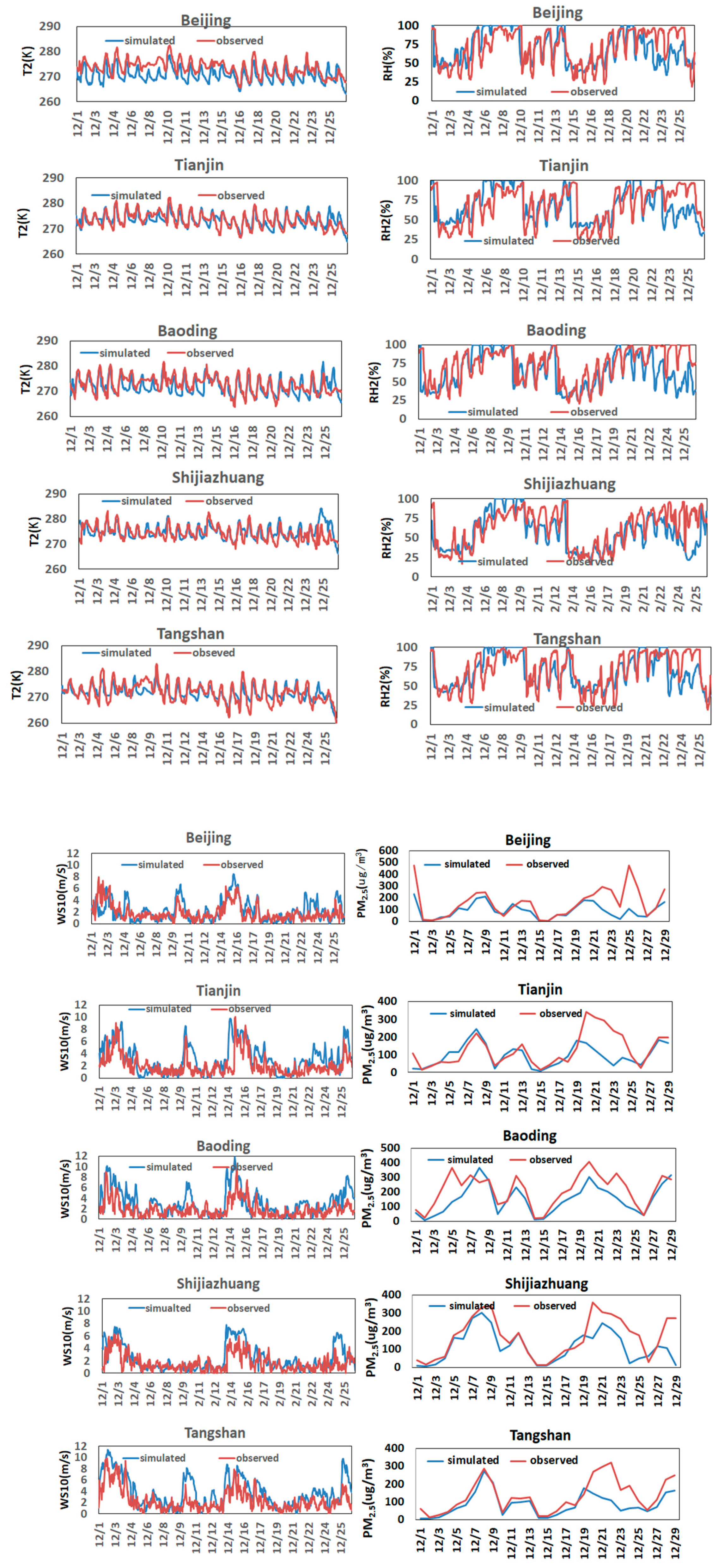
The evaluation statistics of T2 (K), RH2 (%), and WS10 (m s−1) for Beijing, Tianjin, Baoding, Shijiazhuang, and Tangshan are summarized in Table 3. Figure 2 presents the hourly simulated and observed meteorological variables and the PM2.5 results. The WRF-Chem simulation results adequately captured the variations in T2 in these regions, with correlation coefficients of 0.72, 0.75, 0.71, 0.53, and 0.78 in Beijing, Tianjin, Baoding, Shijiazhuang, and Tangshan, respectively. The NMB and NME indicated good model performance for T2. The NMB values of T2 were between −1.00% and 1.00%, and the NME values of T2 were 1.00%, 0.58%, 0.81%, 0.98%, and 0.75% in Beijing, Tianjin, Baoding, Shijiazhuang, and Tangshan, respectively. As shown in Table 3, Beijing, Tianjin, and Tangshan showed the smallest NMB and NME values for the RH simulation. Baoding and Shijiazhuang presented relatively large biases for the RH simulation, and they are located in heavily polluted areas. The RH2 simulation results had correlation coefficients between 0.59 and 0.74. The simulation results adequately captured the variations in WS10. All correlation coefficients were greater than 0.5. However, as the analysis nudging option was not applied in the model, overpredictions occurred for hourly WS10 in the regions, with average bias values between 17.9 and 67.44 at five sites. The evaluation of the PM2.5 concentrations in Beijing, Tianjin, Baoding, Shijiazhuang, and Tangshan is also shown in Table 3. The NMB values for the comparison results of PM2.5 were −41.37%, 24.66%, 28.35%, 30.95%, and −34.79% in Beijing, Tianjin, Baoding, Shijiazhuang, and Tangshan, respectively. The NME values of PM2.5 from the different sites were generally between 32.83% and 43.76%. The correlation coefficients of the PM2.5 concentrations between the simulated and observed values were 0.67, 0.58, 0.80, 0.74, and 0.80 in Beijing, Tianjin, Baoding, Shijiazhuang, and Tangshan, respectively. The model simulation results can clearly represent the air pollution process. The high uncertainty of emission inventories and meteorological simulation results affected the accuracy of the air pollution simulation results. A previous study also showed a large bias during heavily polluted days, which is an inherent characteristic that the model can produce [39]. According to the U.S. Environmental Protection Agency [38], all parameters followed the guidelines, and the WRF-Chem model predicted variables reasonably well in this work.

3.2. ARI Effects of Different PM Components

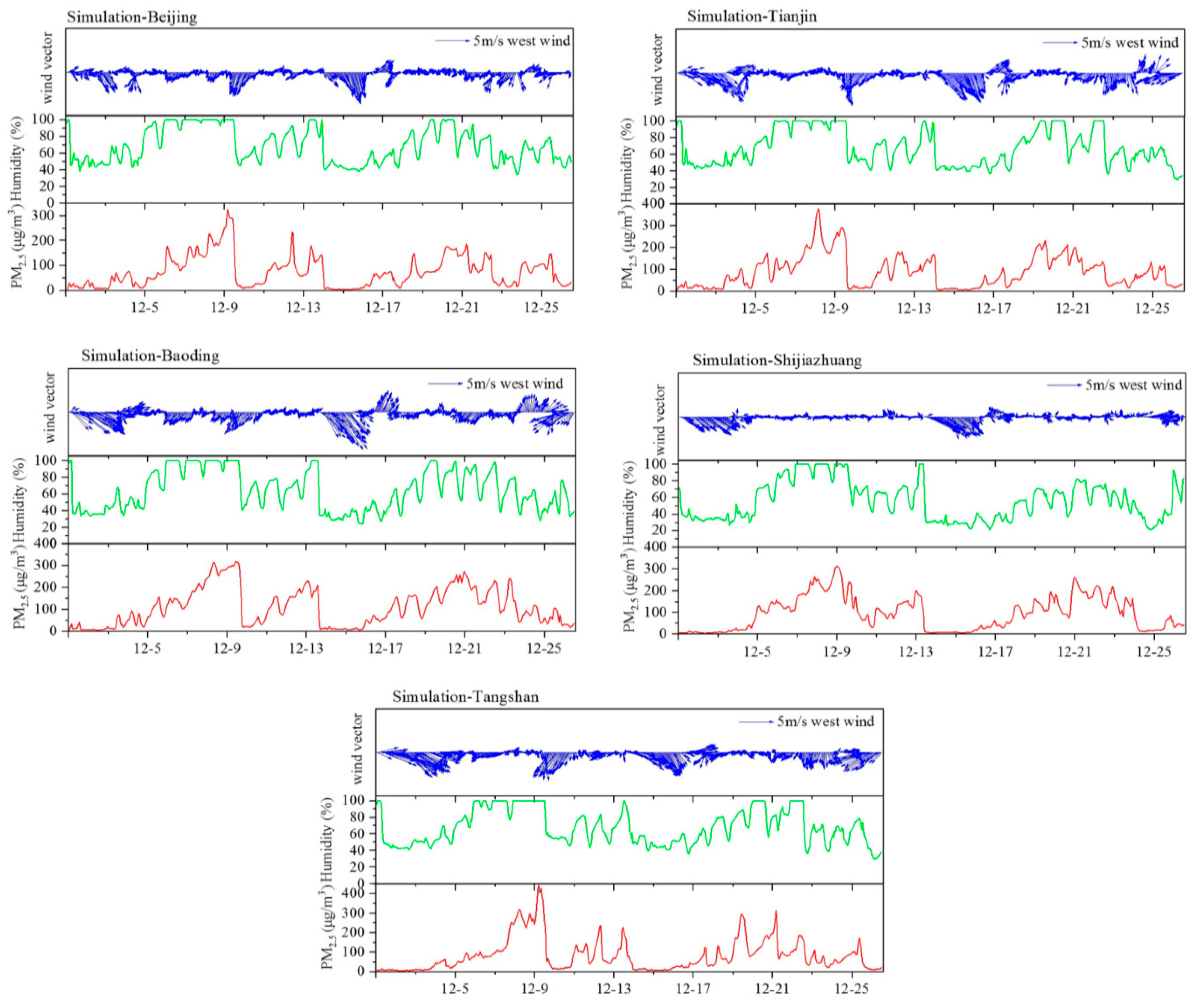
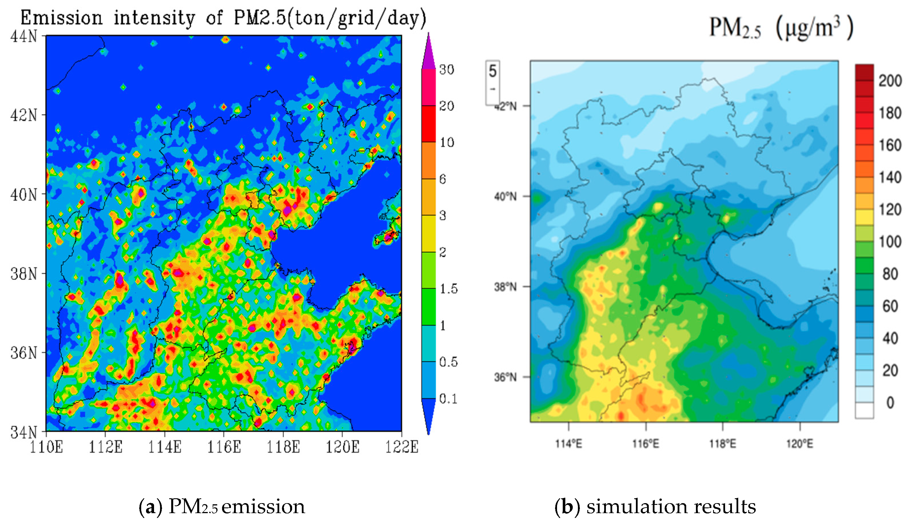
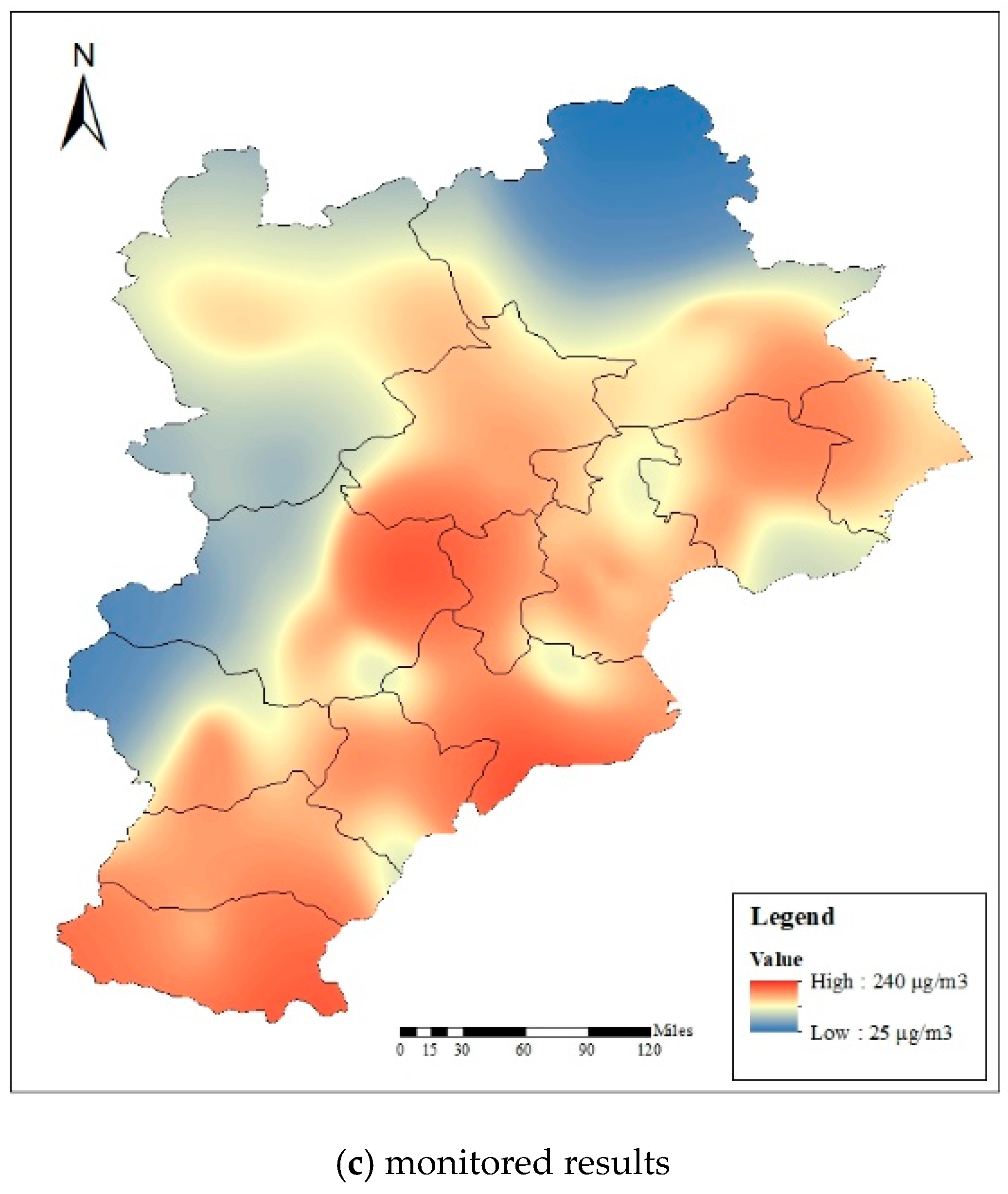
Figure 3 presents the hourly temporal variations in PM2.5 concentration and the meteorological parameters (wind speed and humidity) in Beijing, Tianjin, Baoding, Shijiazhuang, and Tangshan in December 2015. Five pollution episodes occurred in December 2015 in these regions. The figure also shows that PM2.5 concentrations are negatively correlated with wind speed, which contributes to the dispersion of PM2.5 pollutants. PM2.5 concentrations are positively correlated with RH, which means the precursors (SO2, NOx, NH3, and volatile organic compounds (VOCs)) have the tendency to convert to PM2.5 through chemical reactions. Figure 4 shows the spatial distributions of the PM2.5 emission inventory, the mean simulation, and the monitor concentration in the BTH region over the simulation period. The cities of Shijiazhuang, Baoding, and Beijing and the southern part of the BTH region had high pollution emissions and heavy air pollution. Heavy pollution formed in the southern parts of the region (e.g., Shijiazhuang, Xingtai, and Handan) and spread towards the northern parts of the region (e.g., Zhangjiakou and Chengde). Eventually, pollution accumulated in front of the Taihang and Yanshan Mountains in the northern and western parts of the region.
The scenario1 and scenario2 model sensitivity results were compared to examine the ARI effects on meteorological variables (SWDOWN, T2, RH2, and PBLH). The ARI effects caused by NO3, SO42 and BC were also examined by comparing the results of scenario1 with the results of scenario3, the results of scenario1 with the results of scenario4, and the results of scenario1 with the results of scenario5. Based on the PM2.5 standard (75 μg m−3) in China, the ARI effects of PM components under different PM2.5 pollution levels were calculated. Two different PM2.5 pollution levels were examined (i.e., daily PM2.5 concentrations from 0 to 75 μg m−3 and greater than 75 μg m−3).

3.2.1. Downward Shortwave Radiation

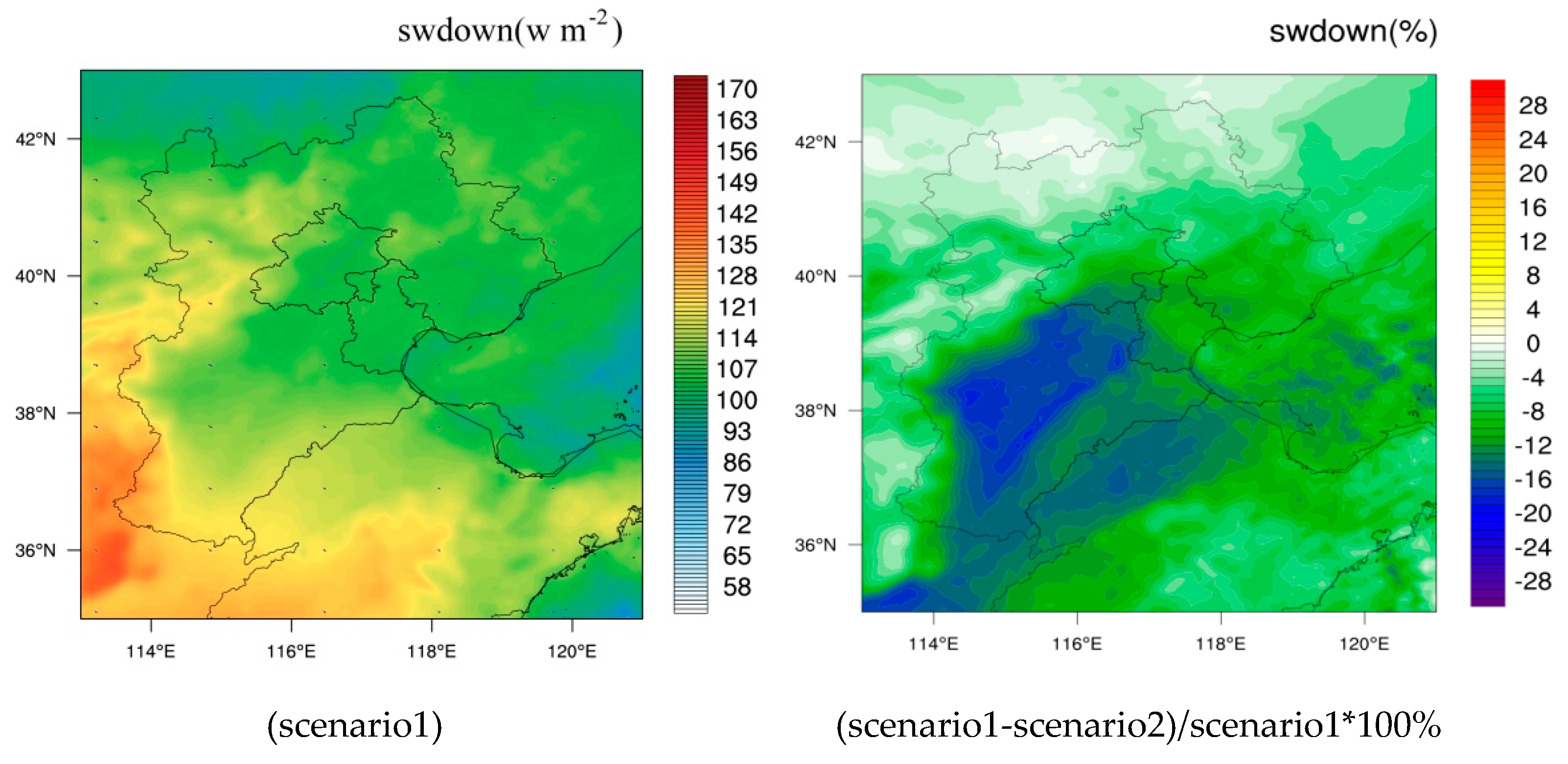
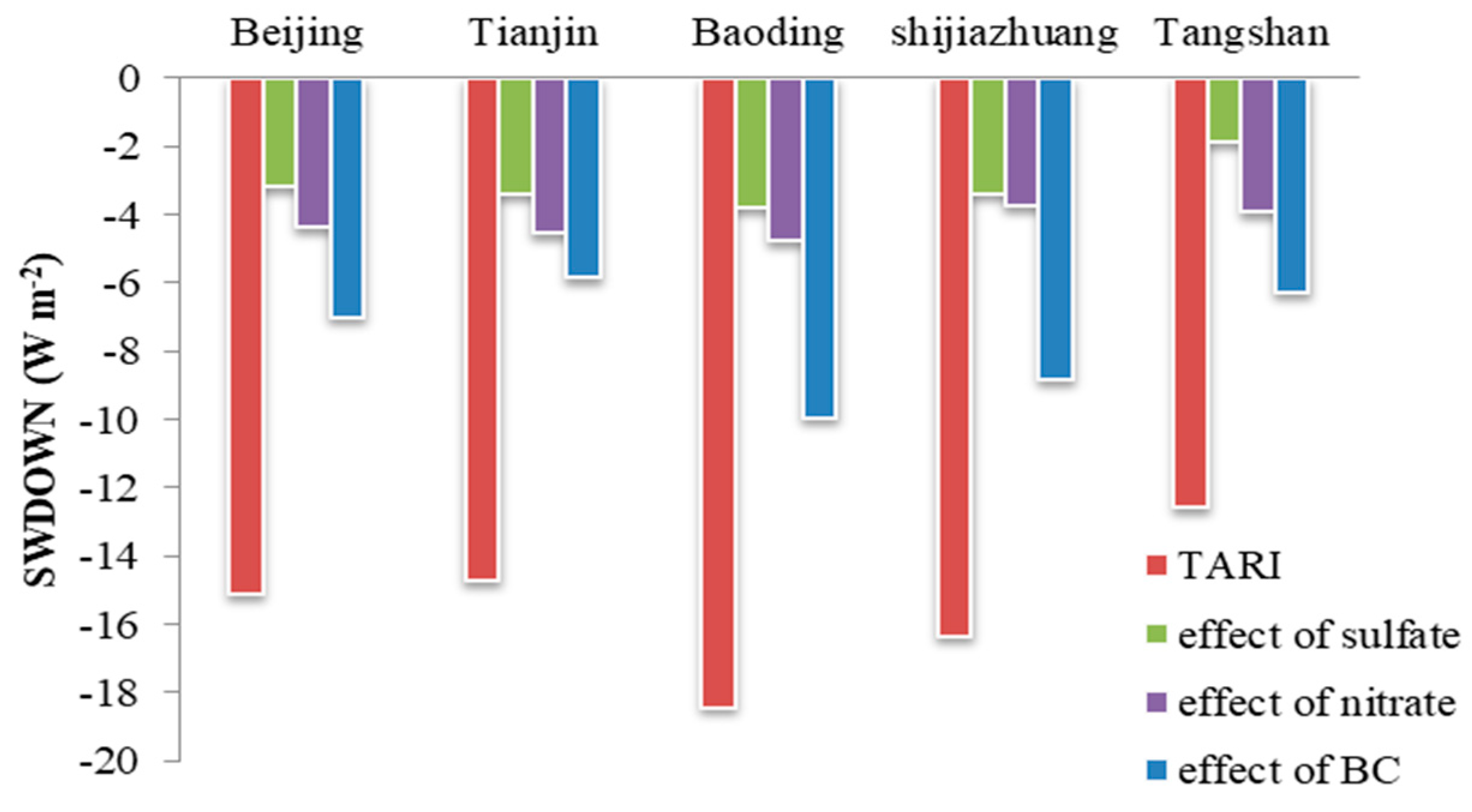
The ARI effects on SWDOWN were examined, whose spatial distributions over the region in December are shown in Figure 5. The left-hand graphs in Figure 5 are the mean distributions of the meteorological variables from the scenario1 simulation. The right-hand graphs in the figure are the relative differences between the scenario1 and scenario2 simulations. The spatial mean contributions of the ARI effect to SWDOWN average were decreases of 14.83 W m−2, 14.48 W m−2, 18.53 W m−2, 16.19 W m−2, and 12.26 W m−2 in Beijing, Tianjin, Baoding, Shijiazhuang, and Tangshan, respectively, over the simulation period. The ARI decreased the SWDOWN in the region, particularly in areas with severe PM2.5 pollution. The SWDOWN decreased in five cities due to the ARI effects of BC, SO42, and NO3, as shown in Figure 6. The BC absorption effect on solar radiation was stronger than the effects of sulfate and nitrate. In December, BC reduced shortwave radiation, of which averages of 7.01 W m−2, 5.86 W m−2, 9.96 W m−2, 8.83 W m−2, and 6.28 W m−2 were observed in Beijing, Tianjin, Baoding, Shijiazhuang, and Tangshan, respectively. The effects of sulfate and nitrate aerosols on solar radiation were relatively mild. The SWDOWN decreases were 4.37 W m−2, 4.55 W m−2, 4.77 W m−2, 3.75 W m−2, and 3.92 W m−2 due to nitrate in Beijing, Tianjin, Baoding, Shijiazhuang, and Tangshan, respectively. The SWDOWN decreased by 3.18 W m−2, 3.39 W m−2, 3.79 W m−2, 3.37 W m−2, and 1.86 W m−2 due to sulfate in Beijing, Tianjin, Baoding, Shijiazhuang, and Tangshan, respectively. The monthly mean ARI effects on SWDOWN under different PM2.5 pollution levels in the five typical cities are provided in Table 4. In the pollution period (PM2.5 concentration > 75 μg m−3), SWDOWN fell by an average of 25.03 W m−2, 5.46 W m−2, 7.61 W m−2, 11.84 W m−2 due to the total ARI (TARI), SO42, NO3, and BC, respectively, in the five cities. During the nonpollution period (PM2.5 concentration < 75 μg m−3), SWDOWN decreased by an average of 5.87 W m−2, 0.77 W m−2, 0.96 W m−2, and 3.33 W m−2 due to the TARI, SO42, NO3, and BC, respectively, in the five cities.

3.2.2. Temperatures at 2 m

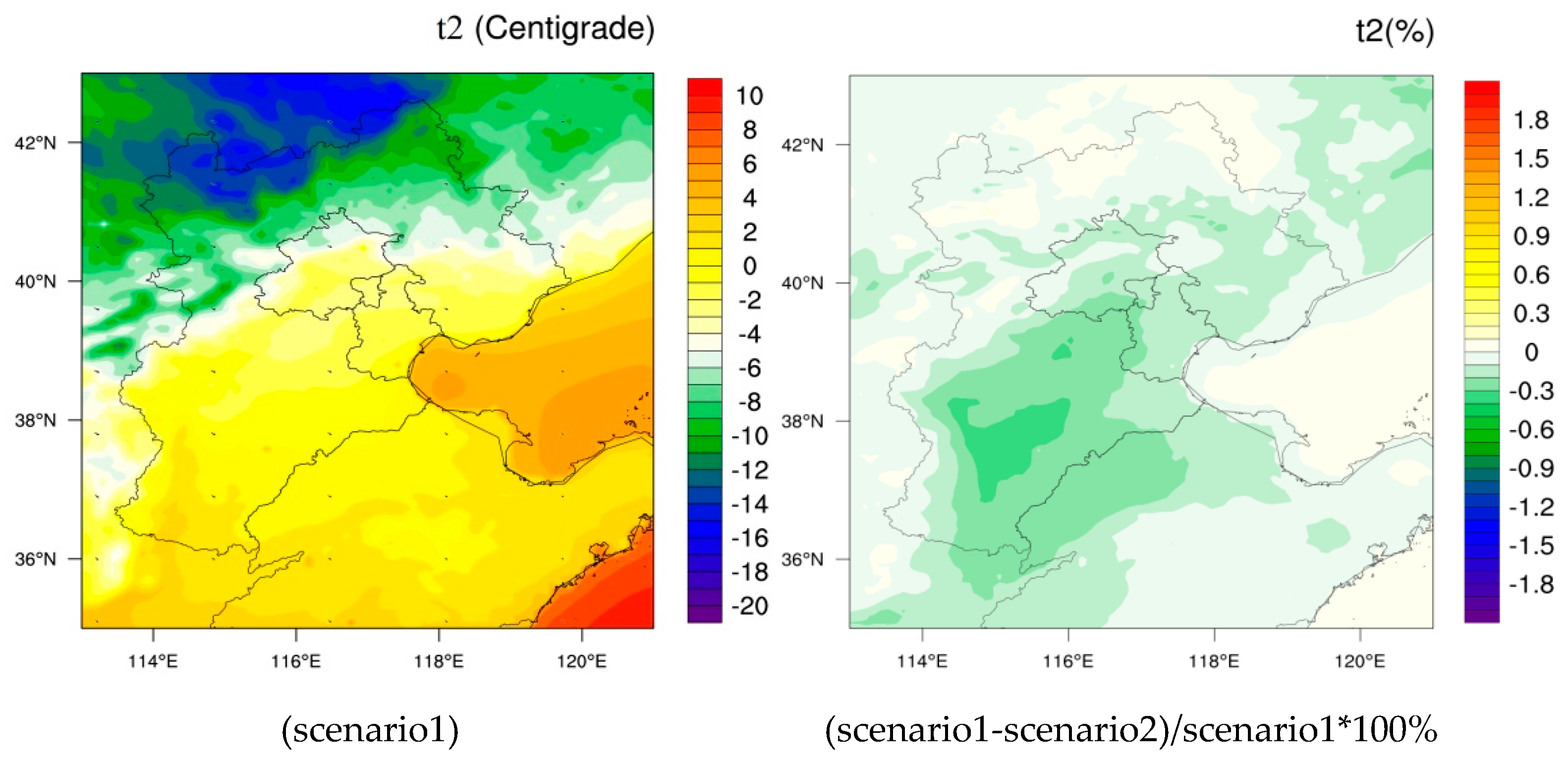
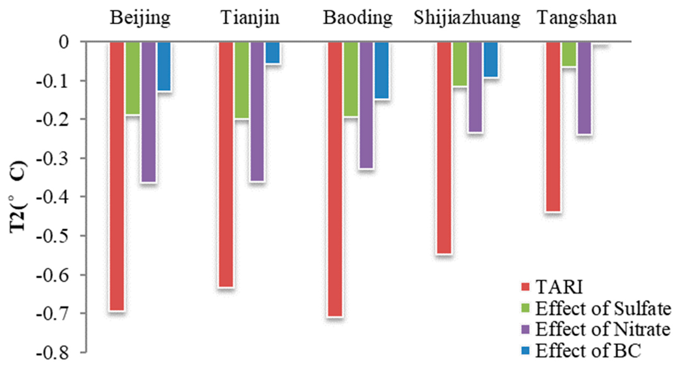
As aerosols reduce incoming solar radiation by scattering and absorption, the surface temperatures decrease. T2 was reduced by up to 1.5 °C in the southern BTH region, of which the cooling effect occurred over most parts of the region, as shown in Figure 7. T2 was reduced by 0.69 °C, 0.63 °C, 0.72 °C, 0.55 °C, and 0.44 °C in Beijing, Tianjin, Baoding, Shijiazhuang, and Tangshan, respectively, over the simulation period, as shown in Figure 7. T2 decreased in the five cities due to the aerosol feedback effect caused by NO3, SO42, and BC, as shown in Figure 8. The temperatures fell by averages of 0.36 °C, 0.36 °C, 0.33 °C, 0.24 °C, and 0.24 °C in Beijing, Tianjin, Baoding, Shijiazhuang, and Tangshan, respectively, due to nitrate. The temperatures fell by averages of 0.19 °C, 0.20 °C, 0.20 °C, 0.12 °C, and 0.07 °C in Beijing, Tianjin, Baoding, Shijiazhuang, and Tangshan, respectively, due to sulfate. BC produces both cooling and heating effects, which was reported by a previous study [12]. On the one hand, when a BC aerosol enters cloud droplet, it enhances the radiation absorption ability of the cloud droplet and leads to a temperature increase. On the other hand, it also promotes the cloud-forming process by acting as cloud condensation nodules and improves cloud reflection. Thus, BC aerosols can cause a surface cooling effect. In this paper, the temperatures fell by an average of 0.13 °C, 0.06 °C, 0.15 °C, 0.09 °C, and 0.00 °C in Beijing, Tianjin, Baoding, Shijiazhuang, and Tangshan, respectively, which was due to BC. The monthly mean ARI effects on T2 under different PM2.5 pollution levels in the five cities are provided in Table 5. During the pollution period, the temperatures fell by averages of 0.94 °C, 0.25 °C, 0.5 °C, and 0.14 °C due to the TARI, SO42, NO3, and BC, respectively, in the five cities. The temperatures fell by averages of 0.28 °C, 0.06 °C, 0.13 °C, and 0.04 °C due to the TARI, SO42, NO3, and BC, respectively, in the five cities during the nonheavy pollution period. The warming effect of BC aerosols caused the temperature to increase by 0.04°C in Tangshan when the PM2.5 concentration was higher than 75 μg m−3.

3.2.3. Plant Boundary Layer Height

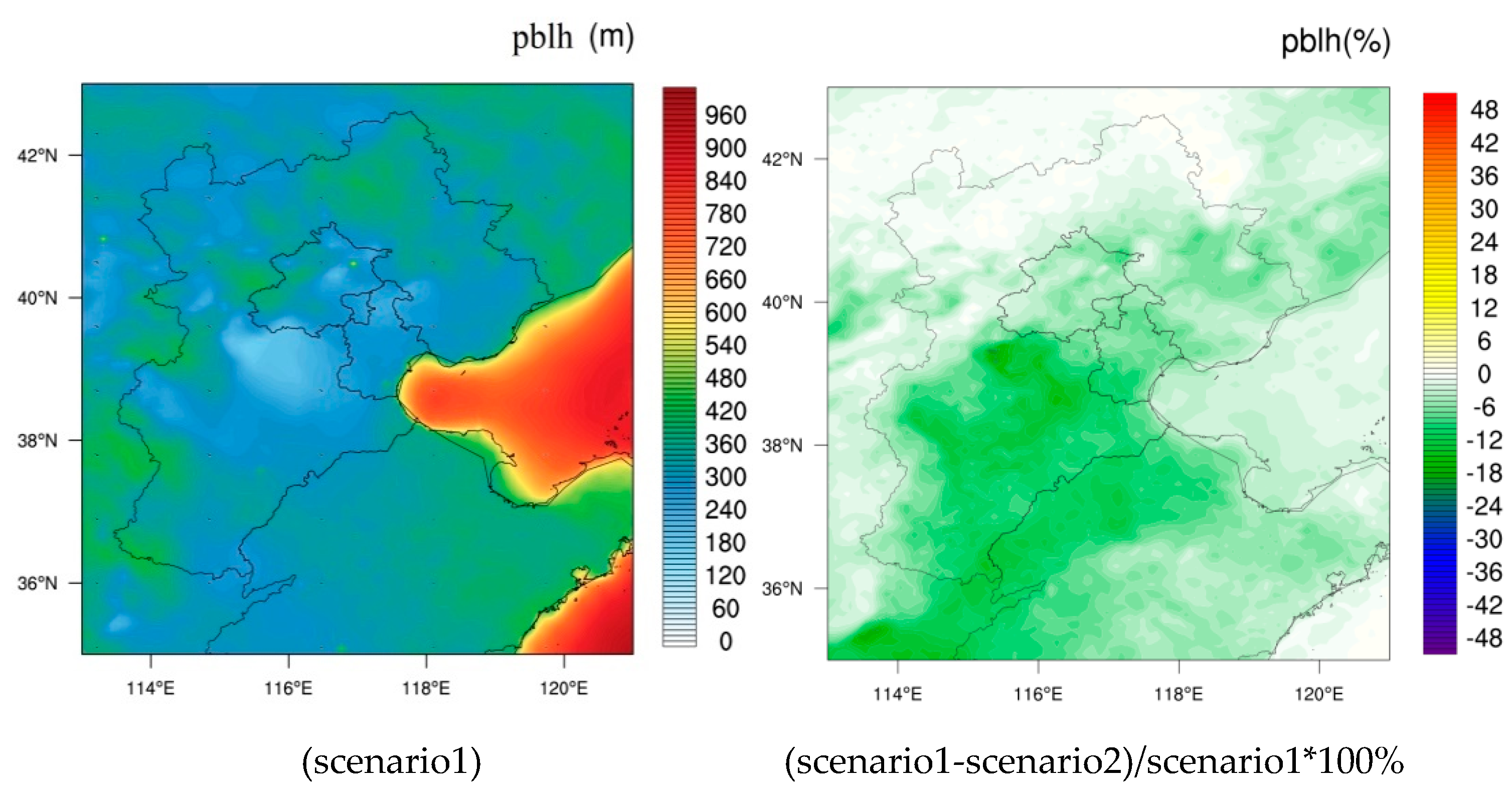
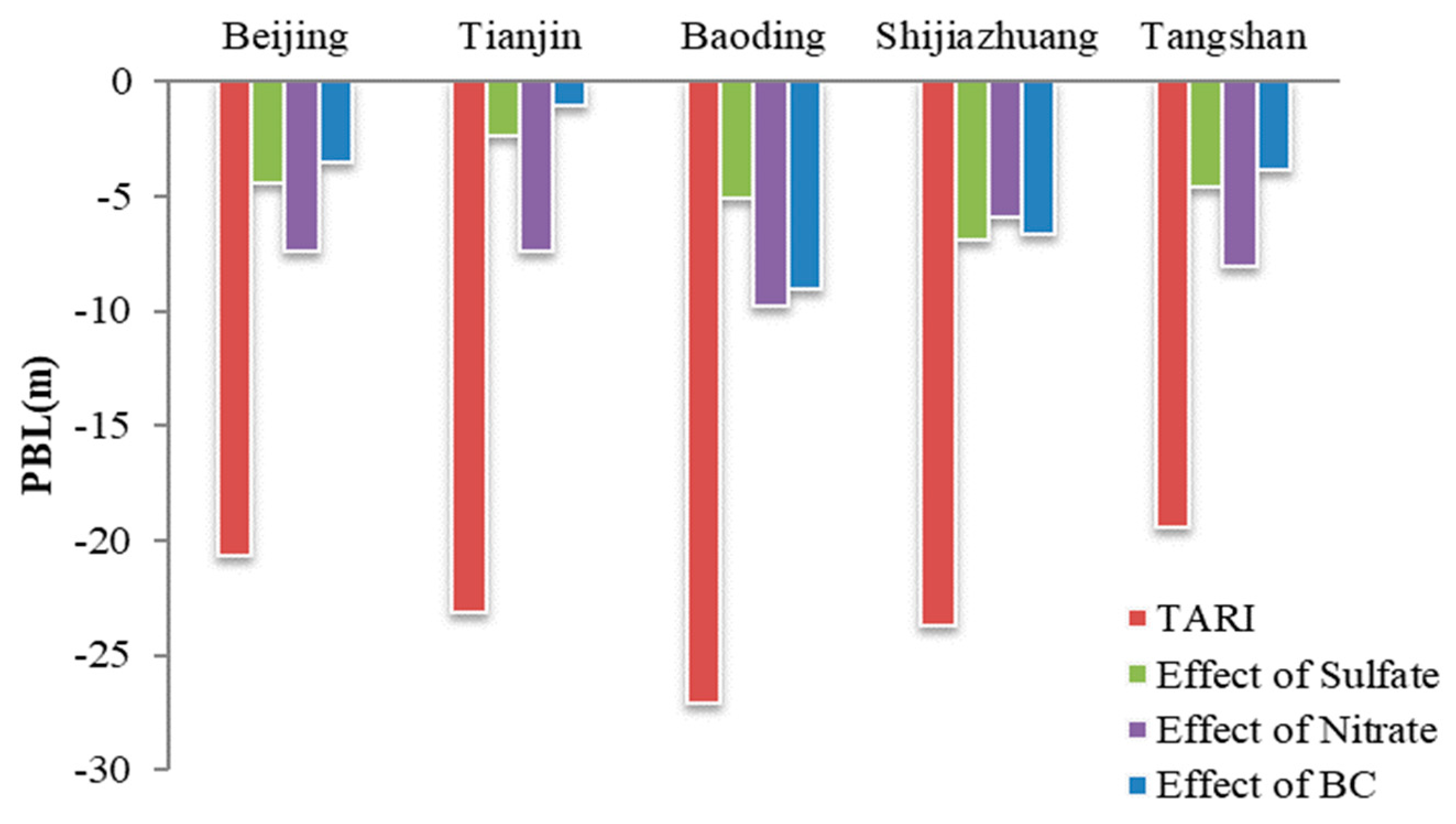
The ARI reduced the PBLH in the region by 5~30 m, as shown in Figure 9. The mean contribution of the ARI to the PBLH in December saw between a 6.56% to 10.3% decrease in the five typical cities in the BTH region. The PBL was reduced by 20.64 m, 23.17 m, 27.08 m, 23.70 m, and 19.40 m in Beijing, Tianjin, Baoding, Shijiazhuang, and Tangshan, respectively. The PBL decreased in the region due to NO3, SO42, and BC emissions, as shown in Figure 10. The PBL fell by averages of 7.41 m, 7.36 m, 9.79 m, 5.95 m, and 8.04 m in Beijing, Tianjin, Baoding, Shijiazhuang, and Tangshan, respectively, due to nitrate. The PBL fell by averages of 4.42 m, 2.34 m, 5.05 m, 6.88 m, and 4.59 m in Beijing, Tianjin, Baoding, Shijiazhuang, and Tangshan, respectively, due to sulfate. The PBL fell by averages of 3.54 m, 1.06 m, 9.09 m, 6.70 m, and 3.89 m in Beijing, Tianjin, Baoding, Shijiazhuang, and Tangshan, respectively, due to BC. The effect of the TARI made the average PBLH decrease by 25.8 m in the region during the PM2.5 pollution period and decrease by 20.07 m during the nonheavy pollution period (shown in Table 6). Sulfate aerosols decreased the average PBLH in six cities by 4.68 m during the PM2.5 pollution period and decreased it by 4.51 m during the non-PM2.5 pollution period. The nitrate and BC aerosols caused the PBLH to decrease by averages of 8.52 m and 7.79 m, respectively, during the pollution period and by 6.96 m and 2.22 m, respectively, during the nonpollution period.

3.2.4. 2-m Relative Humidity

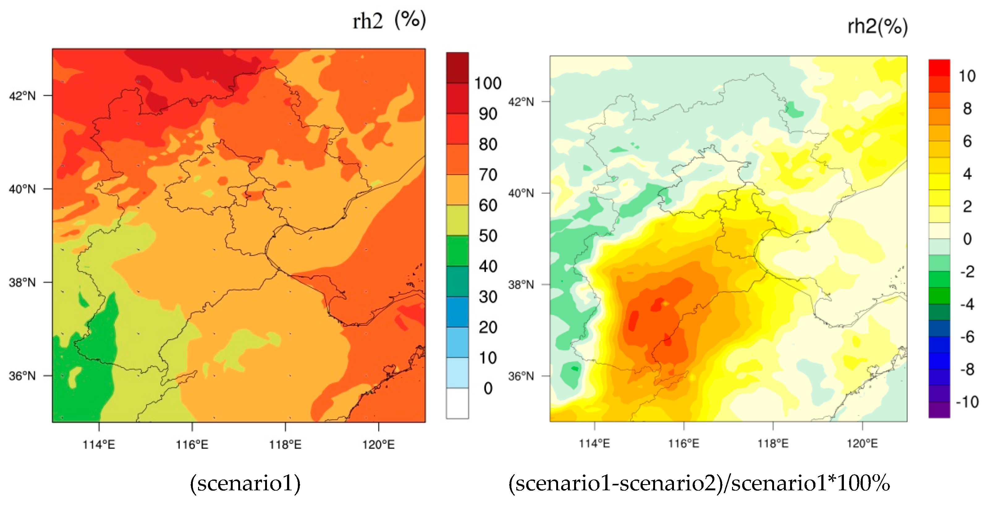
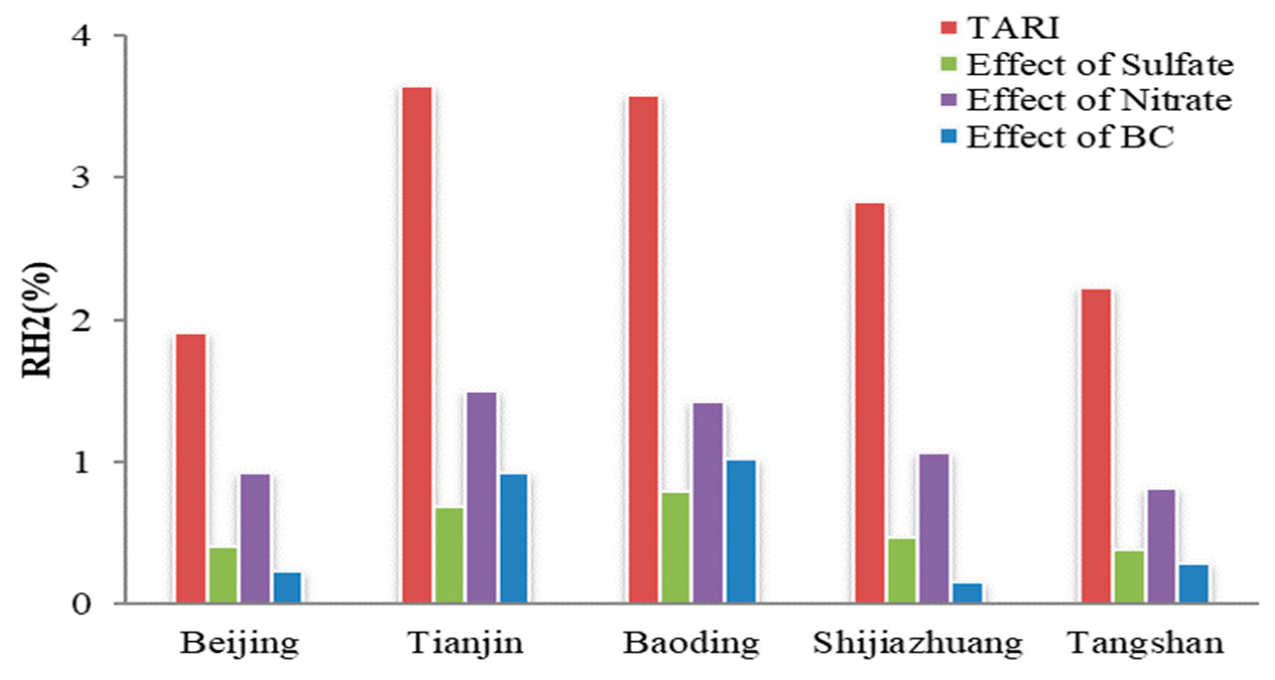
The monthly average RH2 exhibited obvious increases in the middle and southern parts of the BTH region, as shown in Figure 11. In Beijing, Tianjin, Baoding, Shijiazhuang, and Tangshan, the mean spatial contributions of the ARI to RH2 over the simulation period were approximately 1.93%, 3.61%, 3.67%, 2.81%, and 2.22%, respectively. The RH2 increased in the five cities due to the aerosol feedback effects of NO3, SO42, and BC, as shown in Figure 12. Nitrate increased RH2 by averaging 0.92%, 1.50%, 1.42%, 1.07%, and 0.81% in Beijing, Tianjin, Baoding, Shijiazhuang, and Tangshan, respectively. Sulfate increased RH2 by averages of 0.40%, 0.68%, 0.80%, 0.47%, and 0.39% in Beijing, Tianjin, Baoding, Shijiazhuang, and Tangshan, respectively. BC increased RH2 by averages of 0.23%, 0.93%, 1.03%, 0.16%, and 0.28% in Beijing, Tianjin, Baoding, Shijiazhuang, and Tangshan, respectively. The effect of the TARI increased the RH2 in the region by an average of 4.40% during the pollution period and increased that by an average of 1.24% during the nonheavy pollution period (shown in Table 7). Sulfate aerosols increased the average RH2 by an average of 0.80% during the pollution period and 0.07% during the nonpollution period. Nitrate and BC aerosols increased RH2 by averages of 1.69% and 1.05%, respectively, during the pollution period, and 0.53% and 0.05%, respectively, during the nonpollution period.
The results in this paper are similar to those of previous studies. For example, in East China, the monthly mean SWDOWN, T2, and PBLH can decrease up to −12.37 W m−2, −0.24°C, and −31.59 m due to ARIs [40]. Even in the eastern continental United States, the ARI effect decreased the SWDOWN by 11.3 W m−2, the T2 by 0.16 K, and the PBLH by 22.4 m in winter [41].

3.2.5. PM2.5 Concentrations

The ARI reduced the surface temperature, increased RH2, and decreased PBLH, which led to a more stable lower atmosphere. Stable meteorological conditions suppressed the dispersion of air pollutants and increased air quality concentrations. The contributions of ARIs increased the PM2.5 concentration by 1.75 μg m−3, 2.00 μg m−3, 2.10 μg m−3, 1.90 μg m−3, and 3.63 μg m−3 in Beijing, Tianjin, Baoding, Shijiazhuang, and Tangshan, respectively. The effect on the PM concentrations showed negative correlations with SWDOWN, T2, and PBLH. The ARI led to a large increase in air pollution concentration in the middle and southern parts of Hebei Province, where the aerosol anthropogenic emissions are high. In this study, the changes in PM2.5 concentration caused by BC, SO2/SO42, and NOx/NO3 emission reductions were also calculated. We found that BC, SO2, and NOx emission control are an effective way to reduce air pollution. The BC emission reduction decreased the PM2.5 concentration by an average of 6.24 μg m−3 in the five cities or 7% of the PM2.5 concentration in the region. The SO2/SO42 emission reduction had a similar trend, with an average deduction of 35% PM2.5 concentration in the five cities. The NOx/NO3 emission contributed to the PM2.5 decrease by an average of 32 μg m−3 in the five cities, which is a reduction of approximately 34% in the PM2.5 concentration from the scenario1 simulation. If BC, SO2/SO42, and NOx/NO3 emission reduction measures were successfully implemented, the PM2.5 concentration was distinctly reduced, which also proves that under heavy pollution conditions, multipollutant emission collaborative controls are needed.

4. Conclusions

In this study, the WRF-Chem model was used to study the ARI effects of BC, SO42 and NO3 in the BTH region of China. The simulation results of the meteorological variables and PM2.5 concentrations were verified with observation data. If there were ARIs in the simulation, the SWDOWN at the surface decreased and led to a decrease in temperature. As a result, SWDOWN suppressed the development of the PBLH and increased the RH2. In summary, this paper investigated the impact of ARI effects on meteorological variables that affect the stability of the atmosphere. The modeling results showed that the BC effect of absorbed solar radiation was stronger than the scattering effects of sulfate and nitrate. The BC produced both cooling and heating effects, while sulfate and nitrate produced cooling effects in December 2015 in the BTH region. The PBLH decreased and the RH increased in the five cities due to the aerosol feedback effects of nitrate, sulfate, and BC. As the nitrate concentrations were higher than the sulfate concentrations in the BTH region, the aerosol feedback effect of the nitrate concentrations was higher than that of sulfate. By comparing the results from pollution and nonpollution periods, the more pollution there was, the greater the ARI effect on meteorological factors. It was found that if there were ARIs, the PM2.5 concentration in the region would increase. The BC emission reduction measures reduced the PM2.5 concentration by 7% in the region. The SO2/SO42 and NOx/NO3 emission reductions decreased the PM2.5 concentration by averages of 35% and 34%, respectively. Multipollutant emission collaborative control is needed to distinctly reduce the PM2.5 concentration.

Author Contributions

Methodology, X.Z. and J.X.; validation, C.G. and L.L.; formal analysis, W.W.; investigation, X.M.; data curation, H.W., W.Z., and Z.Z.; writing—original draft preparation, W.W.; writing—review and editing, X.M. All authors have read and agreed to the published version of the manuscript.

Funding

This research was supported by State Grid Corporation of China: “Study on the benefit of air environment improvement of “replacing coal with electricity” in typical areas such as Beijing, Tianjin and Hebei” (No. 52010118000C), the National Natural Science Foundation of China (Grant No. 51808549, 21806183), Beijing Major Science and Technology Project (Z181100005418014), and Chinese Academy of Meteorological Sciences Foundation (2018Y001).

Conflicts of Interest

The authors declare no conflict of interest.

References

  1. Santos, D.; Costa, M.J.; Silva, A.M. Direct SW aerosol radiative forcing over Portugal. Atmos. Chem. Phys. 2008, 8, 5771–5786. [Google Scholar]
  2. Dhar, P.; De, B.K.; Banik, T.; Gogoi, M.M.; Babu, S.S.; Guha, A. Atmospheric aerosol radiative forcing over a semi-continental location Tripura in North-East India: Model results and ground observations. Sci. Total Environ. 2017, 580, 499–508. [Google Scholar] [CrossRef] [PubMed]
  3. Obregón, M.A.; Costa, M.J.; Silva, A.M.; Serrano, A. Impact of aerosol and water vapour on SW radiation at the surface: Sensitivity study and applications. Atmos. Res. 2018, 213, 252–263. [Google Scholar] [CrossRef]
  4. Charlson, R.J.; Schwartz, S.E.; Hales, J.M.; Cess, R.D.; Coakley, J.A.; Hansen, J.E.; Hofmann, D.J. Climate Forcing by Anthropogenic Aerosols. Science 1992, 255, 423–430. [Google Scholar] [CrossRef] [PubMed]
  5. Pere, J.C.; Mallet, M.; Pont, V.; Bessagnet, B. Impact of aerosol direct radiative forcing on the radiative budget, surface heat fluxes, and atmospheric dynamics during the heat wave of summer 2003 over western Europe: A modeling study. J. Geophys. Res. Atmos. 2011, 116, D23119. [Google Scholar] [CrossRef]
  6. Boucher, O.; Randall, D.; Artaxo, P. Clouds and aerosols. In Climate Change 2013: The Physical Science Basis. Contribution of Working Group I to the Fifth Assessment Report of the Intergovernmental Panel on Climate Change; Stocker, T.F., Qin, D., Plattner, G., Tignor, M., Allen, S.K., Boschung, J., Nauels, A., Xia, Y., Bex, V., Midgley, P.M., Eds.; Cambridge University Press: Cambridge, UK; New York, NY, USA, 2013. [Google Scholar]
  7. Xing, J.; Mathur, R.; Pleim, J.; Hogrefe, C.; Gan, C.M.; Wong, D.C.; Wei, C.; Wang, J.D. Air pollution and climate response to aerosol direct radiative effects: A modeling study of decadal trends across the northern hemisphere. J. Geophys. Res. Atmos. 2015, 120, 12221–12236. [Google Scholar] [CrossRef]
  8. Guo, J.; Liu, H.; Wang, F.; Huang, J.F.; Xia, F.; Lou, M.Y.; Wu, Y.R.; Jiang, J.H.; Xie, T.; Zhaxi, Y.Z.; et al. Three-dimensional structure of aerosol in China: A perspective from multi-satellite observations. Atmos. Res. 2016, 178, 580–589. [Google Scholar] [CrossRef]
  9. Dong, C.; Matsui, H.; Spak, S.; Kalafut-Pettibone, A.; Stanier, C. Impacts of New Particle Formation on Short-term Meteorology and Air Quality as Determined by the NPF-explicit WRF-Chem in the Midwestern United States. Atmos. Chem. Phys. 2018, 19, 204. [Google Scholar] [CrossRef]
  10. IPCC. Climate change 2007: Synthesis Report. In Contribution of Working Group I to the Fourth Assessment Report of the Intergovernmental Panel on Climate Change; Solomon, S., Qin, D., Manning, M., Eds.; Cambridge University Press: Cambridge, UK, 2007. [Google Scholar]
  11. Ramanathan, V.P.J.; Crutzen, J.T.; Kiehl, D. Rosenfeld. Aerosols, Climate, and the Hydrological Cycle. Sciences 2010, 5549, 2119–2124. [Google Scholar]
  12. Jacobson, M.Z. Atmospheric Pollution: History, Sciences and Regulation; Cambridge University Press: New York, NY, USA, 2002; 399p, ISBN 0521010446. [Google Scholar]
  13. Ma, Y.; Xin, J.Y.; Zhang, W.Y.; Liu, Z.R.; Ma, Y.J.; Kong, L.B.; Wang, Y.S.; Deng, Y.; Lin, S.H.; He, Z.M. Long-term variations of the PM2.5 concentration identified by MODIS in the tropical rain forest, Southeast Asia. Atmos. Res. 2019, 219, 140–152. [Google Scholar] [CrossRef]
  14. MEP. 2017 Air Pollution Prevention and Management Plan for the Beijing-Tianjin-Hebei Region and Its Surrounding Areas. Available online: http://dqhj.mee.gov.cn/dtxx/201703/t20170323_408663.shtml (accessed on 18 August 2018).
  15. Wen, W.; Cheng, S.Y.; Chen, X.F.; Wang, G.; Li, S.; Wang, X.Q.; Liu, X.Y. Impact of emission control on PM2.5 and the chemical composition change in Beijing-Tianjin-Hebei during the APEC summit 2014. Environ. Sci. Pollut. Res. 2016, 105, 432–436. [Google Scholar] [CrossRef] [PubMed]
  16. Wang, G.; Cheng, S.Y.; Lang, J.L.; Yang, X.W.; Wang, X.Q.; Chen, G.L.; Liu, X.Y.; Zhang, H.Y. Characteristics of PM2.5 and assessing effects of emission—Reduction measures in the heavy polluted city of Shijiazhuang, before, during, and after the Ceremonial Parade 2015. Aerosol Air Qual. Res. 2017, 17, 499–512. [Google Scholar] [CrossRef] [Green Version]
  17. Zhang, X.Y.; Wang, Y.Q.; Lin, W.L.; Zhang, Y.M.; Zhang, X.C.; Gong, S.; Zhao, P.; Yang, Y.Q.; Wang, J.Z.; Hou, Q.; et al. Changes of atmospheric composition and optical properties over Beijing 2008 Olympic monitoring Campaign. Bull. Am. Meteorol. Soc. 2009, 90, 1633–1651. [Google Scholar] [CrossRef] [Green Version]
  18. Wang, T.; Nie, W.; Gao, J.; Xue, L.K.; Gao, X.M.; Wang, X.F.; Qiu, J.; Poon, C.N.; Meinardi, S.; Blake, D.; et al. Air quality during the 2008 Beijing Olympics: Secondary pollutants and regional impact. Atmos. Chem. Phys. 2010, 10, 7603–7615. [Google Scholar] [CrossRef] [Green Version]
  19. Xu, W.Q.; Sun, Y.L.; Chen, C.; Du, W.; Han, T.T.; Wang, Q.Q.; Fu, P.Q.; Wang, Z.F.; Zhao, X.J.; Zhou, L.B.; et al. Aerosol composition, oxidation properties, and sources in Beijing: Results from the 2014 Asia-Pacific Economic Cooperation summit study. Atmos. Chem. Phys. 2015, 15, 13681–13698. [Google Scholar] [CrossRef] [Green Version]
  20. Sun, Y.; Wang, Z.F.; Wild, O. “APEC Blue”: Secondary Aerosol Reductions from Emission Controls in Beijing. Sci. Rep. 2016, 6, 20668. [Google Scholar] [CrossRef] [Green Version]
  21. Makar, P.A.; Gong, W.; Milbrandt, J. Feedbacks between air pollution and weather, Part 1: Effects on weather. Atmos. Environ. 2015, 115, 442–469. [Google Scholar] [CrossRef]
  22. Forkel, R.; Werhahn, J.; Hansen, A.B.; McKeen, S.; Peckham, S.; Grell, G.; Suppan, P. Effect of Aerosol radiation Feedback on Regional Air Quality—A Case Study with WRF/Chem. Atmos. Environ. 2012, 53, 202–211. [Google Scholar] [CrossRef]
  23. Giorgi, F.; Bi, X.; Qian, Y. Indirect vs. Direct Effects of Anthropogenic Sulfate on the Climate of East Asia as Simulated with a Regional Coupled Climate Chemistry Aerosol Mode. Clim. Chang. 2003, 58, 345–376. [Google Scholar] [CrossRef]
  24. Zhuang, B.L.; Liu, L.; Shen, F.H.; Wang, T.J.; Han, Y. Semi-direct Radiative Forcing of Internal Mixed Black Carbon Cloud Droplet and Its Regional Climatic Effect over China. J. Geophys. Res. 2010, 115, D00K19. [Google Scholar] [CrossRef] [Green Version]
  25. Yang, X. Intensification of aerosol pollution associated with its feedback with surface solar radiation and winds in Beijing. J. Geophys. Res. Atmos. 2016, 121, 4093–4099. [Google Scholar] [CrossRef]
  26. Quan, J.N.; Tie, X.; Zhang, Q.; Liu, Q.; Li, X.; Gao, Y.; Zhao, D. Characteristics of heavy aerosol pollution during the 2012–2013 winter in Beijing, China. Atmos. Environ. 2014, 88, 83–89. [Google Scholar] [CrossRef]
  27. Gao, Y. Modeling the feedback between aerosol and meteorological variables in the atmospheric boundary layer during a severe fog-haze event over the North China Plain Atmos. Chem. Phys. 2015, 15, 1093–1130. [Google Scholar]
  28. Zhou, M.; Zhang, L.; Chen, D.; Gu, Y.; Zhao, B. The impact of aerosol–radiation interactions on the effectiveness of emission control measures. Environ. Res. Lett. 2019, 14, 02400. [Google Scholar] [CrossRef]
  29. Zaveri, R.A.; Peters, L.K. A new lumped structure photochemical mechanism for large-scale applications. J. Geophys. Res. 1999, 104, 30387–30415. [Google Scholar] [CrossRef]
  30. Zaveri, R.A.; Easter, R.C.; Fast, J.D.; Peters, L.K. Model for simulating aerosol interactions and chemistry (MOSAIC). J. Geophys. Res. 2008, 113, D13204. [Google Scholar] [CrossRef]
  31. Thompson, G.; Field, P.R.; Rasmussen, R.M.; Hall, W.D. Explicit forecasts of winter precipitation using an improved bulk microphysics scheme. Part II: Implementation of a new snow parameterization. Mon. Weather Rev. 2008, 136, 5095–5115. [Google Scholar] [CrossRef]
  32. Chou, M.D.; Suarez, M.J. An Efficient Thermal Infrared Radiation Parameterization for Use in General Circulation Models; NASA Technical Memorandum; NASA Goddard Space Flight Center: Greenbelt, MD, USA, 1994; Volume 3, pp. 1–85.
  33. Mlawer, E.J.; Taubman, S.J.; Brown, P.D.; Iacono, M.J.; Clough, S.A. Radiative transfer for inhomogeneous atmospheres: RRTM, a validated correlated-k model for the longwave. J. Geophys. Res. 1997, 102, 16663–16682. [Google Scholar] [CrossRef] [Green Version]
  34. Hong, S.Y.; Noh, Y.; Dudhia, J. A new vertical diffusion package with an explicit treatment of entrainment processes. Mon. Weather Rev. 2006, 134, 2318–2341. [Google Scholar] [CrossRef] [Green Version]
  35. Fast, J.D.; Gustafson, W.I.; Easter, R.C.; Zaveri, R.A.; Barnard, J.C.; Chapman, E.G.; Grell, G.A.; Peckham, S.E. Evolution of ozone, particulates, and aerosol direct radiative forcing in the vicinity of Houston using a fully coupled meteorology–chemistry–aerosol model. J. Geophys. Res. 2006, 111, D21305. [Google Scholar] [CrossRef]
  36. Tsinghua University. Multi-resolution Emission Inventory for China. 2016. Available online: http://www.meicmodel.org/ (accessed on 18 June 2019).
  37. Zhang, Y.; Kristen, M.O.; Wang, K. Fine scale modeling of agricultural air quality over the southeastern united states using two air quality models. Part II. Sensitivity studies and policy implications. Aerosol Air Qual. Res. 2013, 13, 1475–1491. [Google Scholar] [CrossRef] [Green Version]
  38. US EPA. Guidance on the Use of Models and Other Analyses for Demonstrating Attainment of Air Quality Goals for Ozone, PM2.5, and Regional Haze; U.S. Environmental Protection Agency Office of Air Quality Planning and Standards Air Quality Analysis Division Air Quality Modeling Group Research: Research Triangle Park, NC, USA, 2007.
  39. Wang, L.T.; Wei, Z.M.; Yang, J.Z.; Zhang, Y.; Zhang, F.F.; Su, J.; Meng, C.C.; Zhang, Q. The 2013 severe haze over southern Hebei, China: Model evaluation, source apportionment, and policy implications. Atmos. Chem. Phys. 2013, 13, 28395–28451. [Google Scholar] [CrossRef]
  40. Chen, D.S.; Ma, X.; Xie, X.; Wei, P.; Wen, W.; Xu, T.T.; Yang, N.; Gao, Q.X.; Shi, H.D.; Guo, X.R.; et al. Modelling the Effect of Aerosol Feedbacks on the Regional Meteorology Factors over China. Aerosol Air Qual. Res. 2015, 15, 1559–1579. [Google Scholar] [CrossRef] [Green Version]
  41. Zhang, Y.; Wen, X.Y.; Jang, C.J. Simulating Chemistry-aerosol-cloud-radiation-climate Feedbacks over the Continental, U.S. Using the Online-coupled Weather Research Recasting Model with Chemistry (WRF/Chem). Atmos. Environ. 2010, 44, 3568–3582. [Google Scholar] [CrossRef]
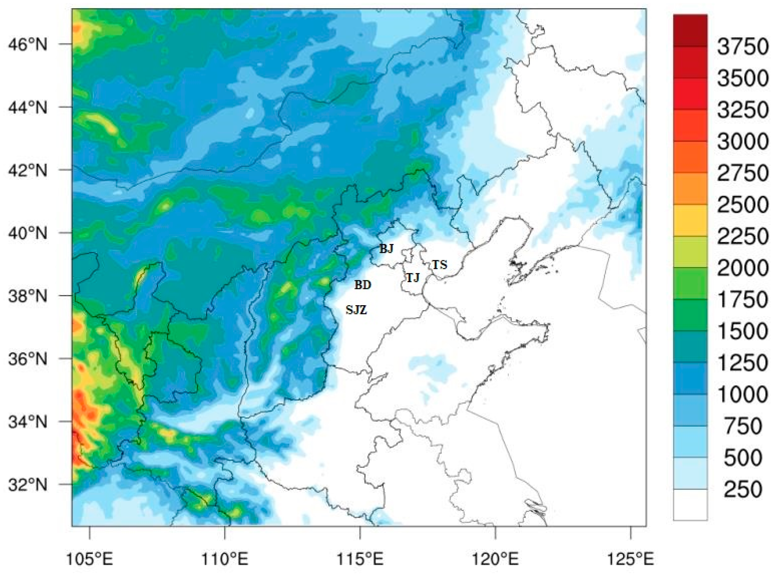
Figure 1. Model simulation domain and topography height (m). (BJ: Beijing; TJ: Tianjin; BD: Baoding; SJZ: Shijiazhuang; TS: Tangshan).
Atmosphere 11 00254 g001
Figure 2. Comparison of temperature at 2 m (T2), relative humidity at 2 m (RH2), wind speed at 10 m (WS10), and PM2.5 between the simulated and observed results.
Atmosphere 11 00254 g002
Figure 3. Hourly PM2.5 concentration and meteorological parameters in the region.
Atmosphere 11 00254 g003
Figure 4. The spatial distributions of the PM2.5 emission inventory, the mean simulation, and the monitored PM2.5 concentration from the scenario 1 simulation. (a) PM2.5 emission, (b) PM2.5 concentration simulation results, (c) PM2.5 concentration monitored results.
Atmosphere 11 00254 g004aAtmosphere 11 00254 g004b
Figure 5. Simulated results of the ARI on SWDOWN. (ARI: aerosol-radiation interaction; SWDOWN: downward shortwave radiation).
Atmosphere 11 00254 g005
Figure 6. Simulated results of ARI effects for different particulate matter components on SWDOWN.
Atmosphere 11 00254 g006
Figure 7. Simulated results of the effects of ARIs under different PM components on T2.
Atmosphere 11 00254 g007
Figure 8. Simulated results of ARI effects under different particulate matter components on T2.
Atmosphere 11 00254 g008
Figure 9. Simulated results of the ARI effects on the planetary boundary layer (PBL).
Atmosphere 11 00254 g009
Figure 10. Simulated results of ARI effects under different particulate matter components on the PBL.
Atmosphere 11 00254 g010
Figure 11. Simulated results of the ARI effect on RH2.
Atmosphere 11 00254 g011
Figure 12. Simulated results of ARI effects under different particulate matter components on RH2.
Atmosphere 11 00254 g012
Table 1. Physical and chemical options included in the study.
Physical and Chemical ProcessesScheme
Microphysics schemeNew Thompson
Shortwave schemeGoddard
Longwave radiation schemeRRTM
PBL schemeYSU
Gas phase chemistryCBM-Z
Aerosol moduleMOSAIC
Aerosols with shortwave radiationMie theory
Table 2. Configurations for the model sensitivity simulation.
RunModel Configuration
Scenario 1Real emission scenario; ARI turned on
Scenario 2Real emission scenario; ARI turned off
Scenario 3No NO3 and NOx emissions; ARI turned on
Scenario 4No SO42− and SO2 emissions; ARI turned on
Scenario 5No BC emission reduction; ARI turned on
Table 3. Statistical results of the simulated and monitored data.
BeijingTianjinBaodingShijiazhuangTangshan
T2 (K)NMB (%)−1.001.00−0.34−0.56−0.10
NME (%)1.000.580.810.980.75
RC0.720.750.710.530.78
RH2 (%)NMB (%)−1.98−1.38−12.59−9.23−3.62
NME (%)19.3523.0721.2222.6318.05
RC0.680.590.640.680.74
WS10
(m s−1)
NMB (%)17.9046.4267.4440.5959.27
NME (%)61.7069.3669.0860.6370.41
RC0.570.650.630.630.78
PM2.5
(μg m3)
NMB (%)−41.3724.6628.3530.95−34.79
NME (%)43.7641.6632.8335.6536.82
RC0.670.580.800.740.80
T2: temperature at 2 m; RH2: relative humidity at 2 m; WS10: wind speed at 10 m; NME: the normalized mean gross error; NMB: normalized mean bias; RC: correlation coefficient (RC).
Table 4. The effects on SWDOWN under different PM2.5 pollution levels.
SWDOWN (W m−2)PM2.5 Concentration (μg m3)BeijingTianjinBaodingShijiazhuangTangshan
TARI>75−26.66−24.45−26.48−25.55−22.02
<75−6.43−5.30−6.99−4.57−6.06
Effect of SO42−>75−6.25−5.98−5.69−5.67−3.73
<75−0.89−0.74−1.02−0.50−0.69
Effect of NO3>75−8.47−8.40−7.45−6.42−7.33
<75−1.25−0.83−0.94−0.41−1.39
Effect of BC>75−12.23−8.14−14.04−13.47−11.31
<75−3.62−3.03−4.12−2.78−3.09
Table 5. The effect on T2 under different PM2.5 pollution levels.
T2 (°C)PM2.5 Concentration (μg m3)BeijingTianjinBaodingShijiazhuangTangshan
TARI>75−1.24−0.94−0.98−0.86−0.70
<75−0.32−0.35−0.29−0.17−0.28
Effect of SO42−>75−0.36−0.34−0.28−0.19−0.10
<75−0.08−0.08−0.06−0.03−0.05
Effect of NO3>75−0.66−0.60−0.45−0.39−0.41
<75−0.17−0.14−0.14−0.05−0.13
Effect of BC>75−0.30−0.08−0.21−0.130.04
<75−0.02−0.03−0.06−0.04−0.04
Table 6. The effects of the ARI on the PBL under different PM2.5 pollution levels.
PBL (m)PM2.5 Concentration (μg m3)BeijingTianjinBaodingShijiazhuangTangshan
TARI>75−23.14−24.09−26.01−32.90−22.88
<75−18.56−23.33−28.73−11.93−17.82
Effect of SO42−>75−4.09−4.50−2.13−8.41−4.25
<75−3.67−0.16−8.81−4.98−4.92
Effect of NO3>75−5.41−9.98−9.04−9.37−8.78
<75−8.99−5.19−10.72−1.67−8.23
Effect of BC>75−7.25−2.97−8.08−13.59−7.06
<75−0.91−0.65−10.302.53−1.77
Table 7. The effect of ARI on RH under different PM2.5 pollution levels.
RH (%)PM2.5 Concentration (μg m3)BeijingTianjinBaodingShijiazhuangTangshan
TARI>753.615.544.954.563.323
<750.701.861.390.781.469
Effect of SO42−>750.731.041.040.710.469
<750.040.070.100.040.079
Effect of NO3>751.502.141.941.711.135
<750.430.790.570.280.588
Effect of BC>751.081.981.420.240.527
<75−0.24−0.010.320.090.079