1. Introduction
The stratosphere is one of the key parts of the atmosphere. One of the most important parameters is temperature, which is interactively connected with radiation, chemistry, and the dynamics of the whole middle atmosphere (stratosphere and mesosphere). Temperature trends are a key parameter of changes in climate. Here, we focus on the winter condition climatology on the Northern Hemisphere, homogeneity analysis, trends in reanalysis, and observations.
Studying the temperature field from observations is a basic diagnostic tool for evaluating climate models or reanalysis (for temperature, e.g., [
1,
2] and for wind, e.g. [
3,
4,
5,
6,
7,
8]). One of the biggest issues with the analysis and validation of the temperature in the middle atmosphere is the uncertainties and homogeneity of observational datasets (e.g., [
9]).
Satellite temperature measurements of the middle atmosphere from the early 1980s can be used for dynamics or trend analysis. One of the longest satellite observation series of stratospheric temperature used in the reanalysis was that of the Stratospheric Sounding Unit (SSU), which is available for 1979–2005 and covers middle and higher stratosphere (see [
10]). For a more recent period (from 1998 till present) we have several possibilities. Ref. [
11] presented the well inter-calibrated and merged SSU and Advanced Microwave Sounding Unit (AMSU) observations available from the NOAA/STAR group. This observation is available for both hemispheres without gaps and is focused mainly on the middle and higher stratosphere, where ground-based observations are missing. Other satellite observations are GPS radio occultation (GPS RO). These temperature observations have been widely used for the middle atmosphere, mainly since 2006. Several studies examined their reliability and comparison with other sources, such as AMSU [
12] or infrared sounding [
11,
13] reported together with [
14,
15] the linear trend over 1979–2015 to be a cooling, which increased with altitude from the lower stratosphere (from ~−0.1 to −0.2 K/decade) to the middle and upper stratosphere (from ~−0.5 to −0.6 K/decade). These studies could be used for comparison with our reanalysis study, especially for the trend analysis because they provide a very wide overview about trends in the stratosphere. The GPS radio occultation and infrared sounding provide another possibility for comparison (see details in [
13]). The AMSU and GPS RO trends of stratospheric temperatures agree well; AMSU displays slightly more negative trends. The 2002–2013 AMSU trend was weak negative [
12]. The Halogen Occultation Experiment (HALOE) trends at 2.0 hPa were of the order of −1.0 K/decade in tropical and subtropical areas and −0.5 K/decade in midlatitudes. Near-global trends at 1 hPa were ~−0.5 K/decade—clearly negative in Southern hemisphere (SH) but slightly positive in Northern hemisphere (NH). Due to the change in the ozone trend, the HALOE trends for 1993–2005 differed from those calculated for 1980–2000 [
16].
Reanalyses are usually used as the true atmospheric state in the stratosphere because direct measurements are not always reliable and available. They provide a spatially and temporally uniform estimate of the atmospheric state, with a wide range of variables, such as temperature, wind, and vorticity available in a standard format [
17]. According to [
18], biases remain between the reanalysis and observed states. Because of the very wide use of reanalyses, we need to quantify and understand these biases precisely. The problem with the reanalyses is that they have different grid resolutions and apply different methods for data assimilation ([
19,
20]). For example, three older reanalyses (National Centers for Environmental Prediction (NCEP)/National Center for Atmospheric Research (NCAR), ECMWF re-analysis (ERA-40), and Japanese 25-year Reanalysis (JRA-25)) using 3D-VAR, show a generally stronger meridional circulation in the stratosphere than newer ones (NCEP/Climate Forecast System Reanalysis (CSFR), ERA-Interim, or JRA-55), which use the 4D-VAR method [
21]. Ref. [
22] analyzed the representation of the stratospheric zonal wind in nine reanalyses and found various problems. Ref. [
20,
23] also reviewed several issues, which should be taken into account when using the reanalysis data for climate or trend studies. The problem of using reanalyses for trend analyses was discussed by some authors (e.g., [
24,
25]), but as [
4,
26] showed, the differences of the temperature anomalies (or wind characteristics) among various ground or satellite observations for the 10 hPa level are generally small in middle and higher latitudes, and discontinuities found in the time series of the reanalyses are not crucial [
18] compared six reanalyses with different satellite observations. They presented several methods of how we can compare the reanalyses with the satellite observations.
Ref. [
16] used ERA-Interim (ERA-I), Modern Era-Retrospective Analysis (MERRA2), and European Center for Medium-Range Weather Forecast Reanalysis (ERA5) for 2002–2017. They found biases in the reanalyses for the linear trends of temperature, since they were affected by the discontinuities in assimilated observations and methods. Such biases can be corrected and the estimated trends can be significantly improved. ERA5 is significantly improved compared to ERA-I and shows the best agreement with the GPS RO temperature. The stratospheric temperature decreases at a rate of 0.1–0.3 K/decade, which is most significant in SH, whereas positive temperature trends are seen in the tropical lower stratosphere (100–50 hPa). As for ozone trends, large biases exist in reanalyses, and it is still challenging to perform trend analysis based on reanalysis ozone data (e.g., [
16,
27]).
A comparison of various reanalyses at higher levels showed that the largest differences in global mean temperatures between reanalysis datasets occur above 10 hPa, with several relatively large changes coincident with changes in the global observing system ([
23,
28]). The temperature trends in reanalyses also show changes of trend patterns in the mid-1990s at least in some areas. According to Leroy et al. (2018), [
13], a comparison of ERA-Interim, MERRA, and MERRA2 versus GPS RO and Atmospheric Infrared Sounder (AIRS) (satellite observations) showed that the retrieved and reanalyzed temperature trends in the lower to middle stratosphere agree within 0.05 K/year. The disagreement between trends from the reanalyses in the upper stratosphere is 0.2 K/year, even though all are anchored to the same radiance measurements, whose weighting functions are peaked near 1.5 hPa. A bias is incurred in GPS RO-retrieved temperatures between the Challenging Minisatellite Payload (CHAMP) and Constellation Observing System for Meteorology, Ionosphere, and Climate (COSMIC) GPS RO missions due to the differing levels of signal noise [
13].
The ERA5 and MERRA2 are the two newest reanalyses that were released; this is why it is necessary to evaluate them, find where the main discontinuities in the time series are, and afterwards, we can decide if it is possible to use them for the trend analysis, which is the aim of this study. Here, we analyze the temperature climatology and trends from the reanalyses ERA5, MERRA2, the GPS RO observations, and several radiosondes to show if the new reanalysis represents reality satisfactorily. The discussion about climatology (discontinuities in time series) versus the trend of selected grid point or trends from GPS RO (even if only since 2006) will bring a new insight into the problem of when it is possible to use reanalyses for trend studies and where the limits lie.
2. Data and Methods
We used the European Centre for Medium-Range Weather Forecasts (ECMWF) reanalysis ERA5, of which the detailed description can be found in ERA5 data documentation, available online: [
29] downloaded from [
30], the Modern Era Retrospective-analysis for Research and Applications (MERRA2, details in [
22]), downloaded from [
31]. As observations, we used data from radiosondes from [
32]. The global positioning system (GPS) radio occultation (GPS RO) technique is an active limb-sounding observation of the Earth’s atmosphere, using a GPS receiver onboard a low Earth orbit (LEO) satellite. Since the observation data taken by such techniques have high accuracy and excellent height resolution, they are very useful for analyzing atmospheric structures, including small-scale vertical fluctuations in the troposphere and stratosphere. The vertical resolution of the geometrical optics (GO) method [
33] in the stratosphere is about 1.5 km due to Fresnel radius limitations, but full spectrum inversion (FSI) [
34] can provide superior resolutions. The archived GPS RO data have been calculated by applying FSI to COSMIC GPS RO profiles at altitudes from ground level up to 30 km. We used the COSMIC GPS RO profiles available at the University Corporation for Atmospheric Research (UCAR) home webpage [
35].
The MERRA2 and ERA5 are available for the period from 1980 till present. The AMSU data used for comparison is available from 1998 and the radiosonde observations at 70, 30, and 10 hPa are partly available from 1980. GPS RO is available from 2004, but we used the period 2006–2018 because, for this period, the GPS RO data are more reliable, especially for the stratosphere (in our case, up to 10 hPa). MERRA2 has the resolution of 0.5° in latitude and 2/3° in longitude. ERA5 has the resolution of 0.75° × 0.75°, and finally, for AMSU and GPS RO, 2.5° × 2.5°. Because we compared the main features and not the fine details, a different grid resolution should not affect our results, but we used the 2.5° × 2.5° resolution for the reanalyses, as well as GPS RO. The reanalyses are available up to 1 hPa (MERRA2 up to 0.1 hPa).
We analyzed each grid point, which meant that we did not use any spatial (longitudinal or latitudinal) averages, because, during every averaging, some information was lost. For each grid and each pressure level, its individual temperature time series was used. The Pettitt homogeneity test [
36] was applied to each grid point to look for a discontinuity. This method is widely used for testing the homogeneity of datasets (e.g., [
37]). In each grid point, the Pettitt test estimated only one main (the biggest) discontinuity, so this procedure was not able to detect multiple discontinuities. We searched for the temporal occurrence of discontinuity so that we were able to detect the discontinuity occurrence in any year. We were also interested in the spatial distribution of the discontinuities. The Pettitt test showed us the year in which the main discontinuity in the time series occurred, but not how big it was or how it could affect the trends. Because of this, we had to apply a variance condition, which compared the variance of the time series and height of the jump. The details of this method can be found by [
27]. We also computed the climatology and temperature trends of MERRA2, GPS RO, and ERA5 for the period 2004–2018 for comparison. Then, we tried to identify the discontinuities in the time series of the MERRA2 and ERA5 computing trend for the periods where we varied their last year. The jumps in this series could also indicate the discontinuities of the time series.
3. Results
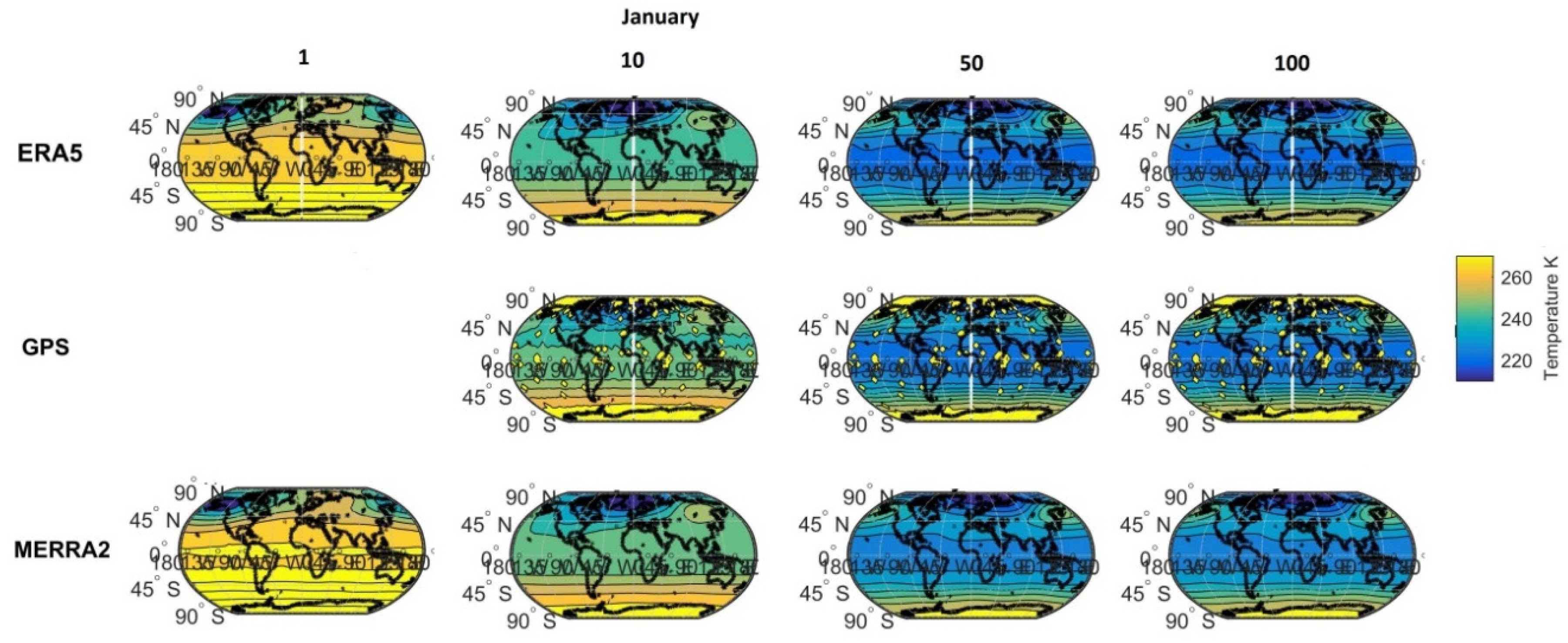
Figure 1 and
Figure 2 show the temperature climatology of two reanalyses (ERA5 and MERRA2) and the GPS RO for December and January during the period 2004–2018 at several pressure levels, from 1 to 100 hPa. We see a very good agreement for the main features as cold areas over the North Pacific (about 230 K) at 1 hPa in December and January. At 10 hPa, there was a cold area over the North Atlantic (210 K) and warmer areas over Asia (about 245 K) in January, but in December, these warm areas were not visible. The same structure as at 10 hPa can be seen at 50 hPa, but the difference between the cold and warm areas was bigger than at 10 hPa, and this feature was visible for both of the analyzed months. We also observed colder air in the tropics (200 K). At 100 hPa, the warm area shifted over the North Pacific and was the main feature in the polar region. Very cold air occurred over the tropics (190 K). This was connected with the tropical upwelling from the troposphere. We found some differences in amplitude, especially at 100 hPa in warm areas, where ERA5 reanalysis and GPS RO were about 3 K warmer than MERRA2. These differences should be taken into account in the detailed analyses.
Now, we move to the homogeneity analysis.
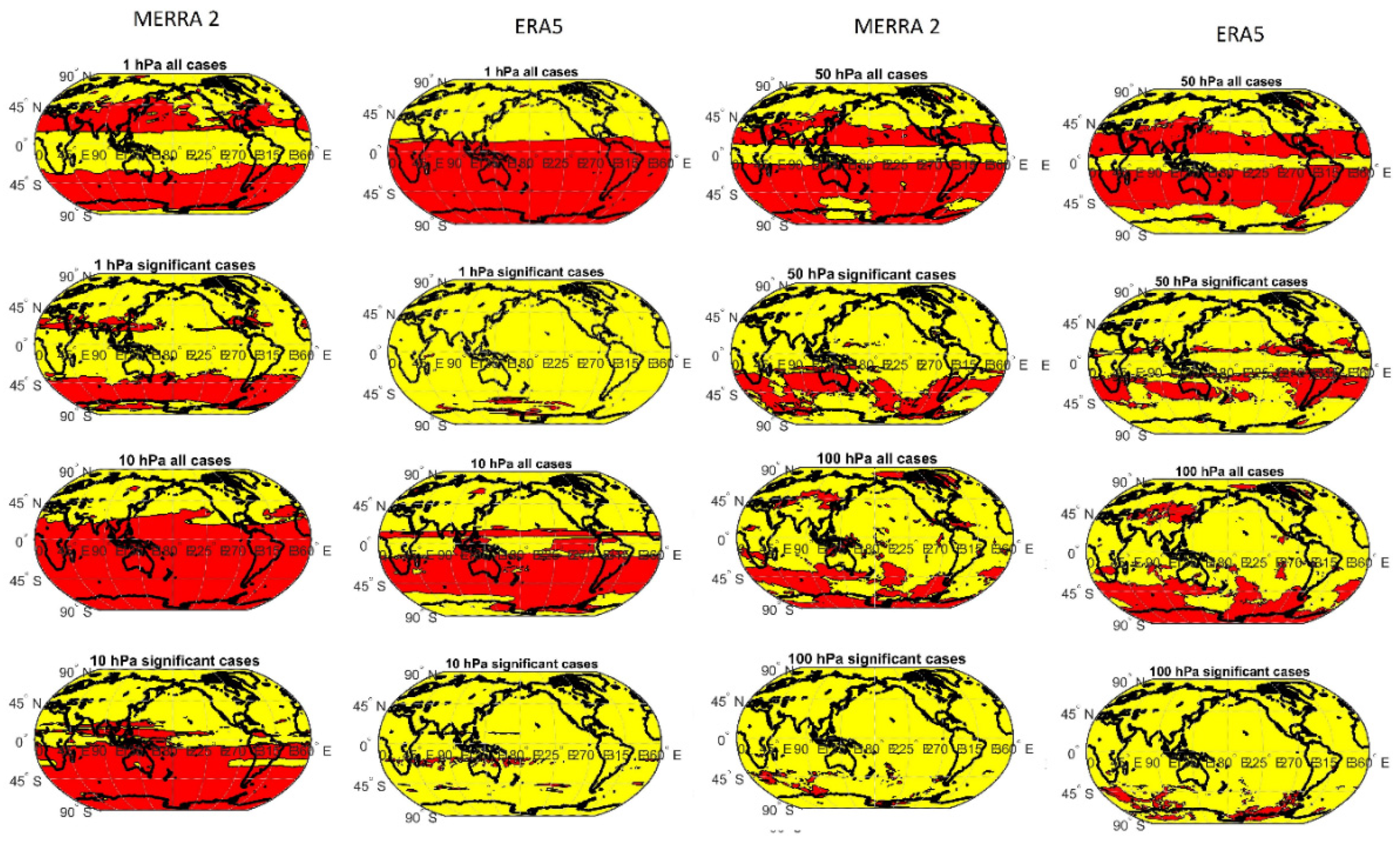
Figure 3,
Figure 4 and
Figure 5 show the analysis of the temperature time series for four pressure levels: 1, 10, 50, and 100 hPa in January and February. We used the Pettitt homogeneity test for the time series 1980–2018 (monthly mean data) and looked for the discontinuities in them for every grid point.
Figure 3 shows the distribution of inhomogeneities in January for the MERRA2 and ERA5 reanalyses. At 1 hPa, we found that for ERA5, across almost the whole Northern Hemisphere, there were no discontinuities, while for MERRA2, we found discontinuities in the middle and lower latitudes of the Northern Hemisphere instead of the tropics (in all cases). When we applied the variance condition, the discontinuities in ERA5 almost disappeared (only small areas in high latitudes of the Southern Hemisphere remained). For MERRA2, the significant cases remained on the Southern Hemisphere and almost disappeared on the Northern Hemisphere.
The results for 10, 50, and 100 hPa are very similar for both reanalyses if we focus on the all cases. At 10 hPa, almost the whole Southern Hemisphere and partly the middle and low latitudes of the Northern Hemisphere were affected by the discontinuities (10 and 50 hPa). At 100 hPa, the small areas with inhomogeneities were randomly distributed over the whole globe. The difference between MERRA2 and ERA5 can be observed when we apply the variance conditions. At 10 hPa especially, there were almost no significant cases for ERA5, but for MERRA2, the area of significant cases covered the whole Southern Hemisphere. At 50 hPa, the significant cases occurred only on the Southern Hemisphere in the middle and higher latitudes. At 100 hPa, both reanalyses show that the time series were not affected by significant discontinuities, which one can expect, because, for this, the pressure levels had much more input datasets than for the stratosphere.
Figure 4 shows a histogram of grid points where the test identified discontinuity. This figure will help us to specify when we find the main peak of discontinuities. Again, we show all cases and significant cases. At 1 hPa, we can see a different distribution for ERA5 and MERRA2. For MERRA2, the main peak can be identified around 2000, which could be connected with the transition from TIROS Operational Vertical Sounder (TOVS) to Advanced TIROS Operational Vertical Sounder (ATOVS), but for ERA5, the first peak is again in 1999, while the main peak is around 2008. If we apply the variance condition, the main peak for MERRA2 remains around 2000; for ERA5, the main peak disappears completely, and only a few significant cases can be seen around 1999. At 10 hPa, there is no main peak, but the jumps are distributed through a long period (1985–2005), which could indicate that the main discontinuity is not connected with a specific situation. Again, if we look at significant cases for MERRA2, there is almost no change, but for ERA5, they almost disappear. The same distribution shows the results for 50 and 100 hPa. We could not identify any main peak; the discontinuities appeared throughout 1986–2010. The difference from 10 hPa was that the significant cases were very similar for both reanalyses, and the distribution of jumps was very similar to all cases, but the number of cases was reduced.
Figure 5 shows the same results as
Figure 3 but for February. At 1 hPa, we can see very similar results as for January. All cases for MERRA2 indicate the discontinuity in the middle and higher latitudes of the Southern Hemisphere and the partly lower latitudes of the Northern Hemisphere, while ERA5 reduced the area with discontinuities southward from 30° S. The results were almost the same for significant cases. For ERA5, there were almost no discontinuities, but for MERRA2, the discontinuities remained even in the Northern Hemisphere, whereas in January, the significant cases in the Northern Hemisphere almost disappeared.
We observed very similar results for MERRA2 at 10 hPa, only the significant area was much smaller in February than in January. ERA5 revealed different results. The area of discontinuities was much smaller for all cases in February than in January. The significant case results showed almost no discontinuities for both months. If we look at the results for 50 and 100 hPa, we can see only small differences between January and February.
Figure 6 shows an overview of the vertical profiles of the occurrence frequency of discontinuities for both reanalyses in January and February, from 500 hPa to 1 hPa. The results for both months are very similar. The ’all cases’ analysis shows that, up to 100 hPa, the jumps occurred in around 30% of all grid points, and the MERRA2 and ERA5 profiles agreed well. If we look at higher pressure levels, the number of jumps increased up to 80% at 5 hPa. Only for ERA5 at 20 and 10 hPa did it rapidly decrease in January to 25%, and in February, less than 15%. From 5 hPa, the ratio again rapidly decreased for both reanalyses in both months to the value of about 40%. The significant case analysis copied the vertical profile of the previous analysis but the values were much smaller, as expected based on previous paragraphs. Up to 100 hPa, the value was around 5%, and it increased mainly for MERRA2 up to 5 hPa, where it reached 50%. ERA 5 showed almost 0% at 10 hPa and 1 hPa, but the maximum of 40% was reached at 3 hPa.
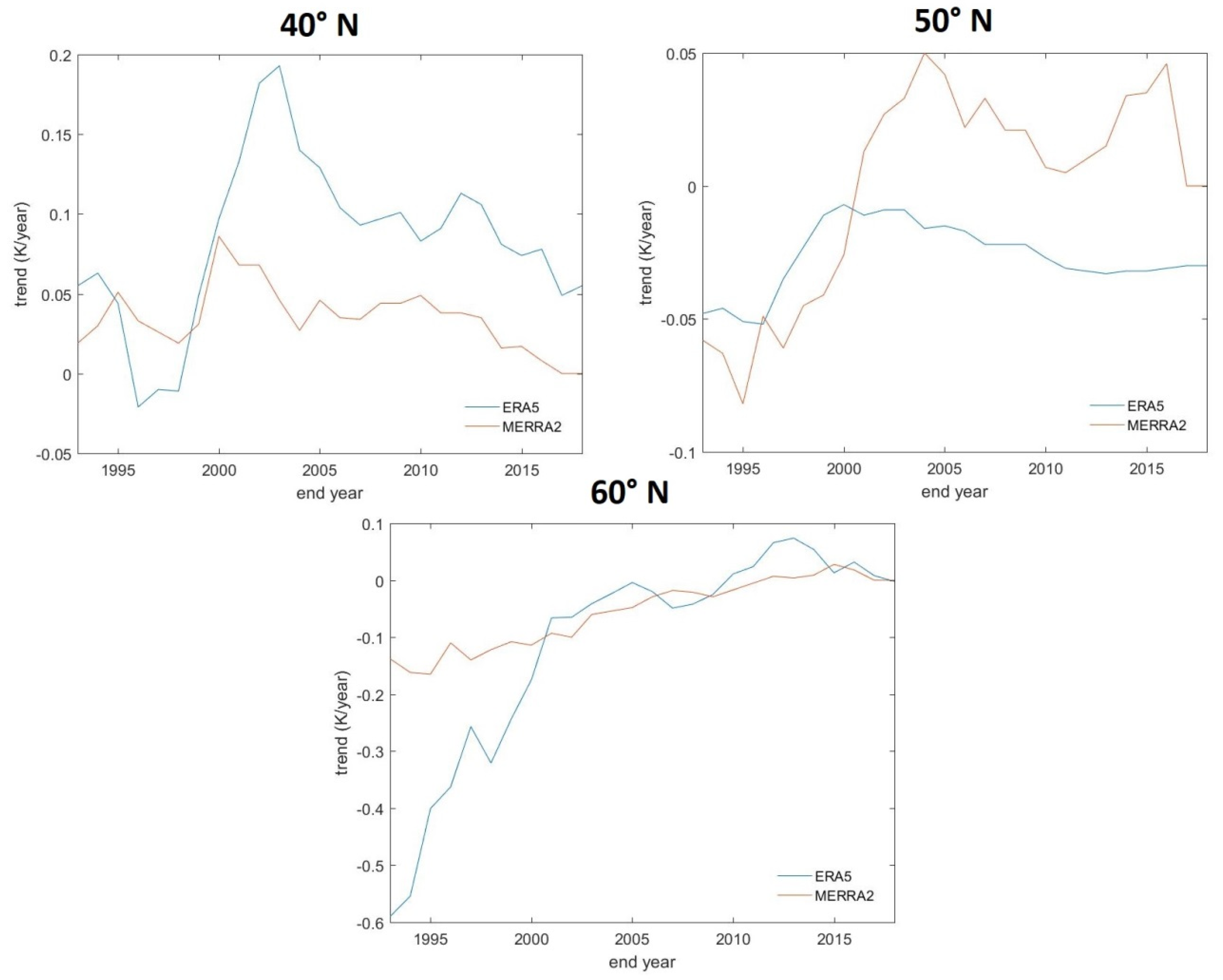
Figure 7 shows a comparison of trends for ERA5 and MERRA2 at 10 hPa. These figures illustrate how the temperature trends change with different lengths of the period (the beginning of the period is set to 1980, and the end year changes from 1993 to 2018) for 40°, 50°, and 60° N. At 40° N, we identified the main jump after 2000 for MERRA2, which could be connected with the changes from TOVS to ATOVS, and in 2003 for ERA5, which need to be studied in more detail. For 50° N and 60° N, the results are quite different than for 40° N. The main jumps occurred after 1998 for ERA5 for both latitudes and in 2005 for MERRA2 (only for 50° N). We are unable to determine the reason for these changes and they must be studied in more detail in the future. The general weakening of trends in more recent years is at least partially due to the weakening/reversal of ozone trends.
All previous results show that we can identify some discontinuities in the time series, but the question as to whether these discontinuities can affect the trends can only be answered if we compare the trends from reanalyses and direct satellite observations. Unfortunately, we do not have reliable direct observations without jumps or missing data. Because of this, we tried to compare the trend from the reanalyses and GPS RO for the period 2004–2018. This comparison may provide the answer if we are able to trust the trend analyses from the reanalyses of at least the last two decades.
Figure 8 and
Figure 9 show the temperature trends in December and January at several pressure levels derived from ERA5, MERRA2, and GPS RO. The results in January show that the behavior of two reanalyses was very similar for all pressure levels, where we found negative trends over the polar regions from 10 hPa to 100 hPa and positive trends over Europe and the North Atlantic at 1 and 10 hPa. If we compare these results with GPS RO, we can see very strong agreement in the main features at the Northern Hemisphere. The comparison of trends agrees well even in December, but we found a different trend distribution here. There were two cores at 50 and 100 hPa and negative trends over the Northern Atlantic and Siberia. A positive trend was found over North America at 10 hPa.
4. Discussion
In this paper, we focus mainly on the data quality of the two newest reanalyses, ERA5 and MERRA2, in terms of discontinuities in the temperature data series. These two reanalyses are usually used as observations or for the validation studies in the stratosphere. Because of this, we need to know if there are some discontinuities/jumps in the time series. We used the Pettitt test to identify the main jumps, but we also applied the variance condition, which was used for the same problem with the ozone [
27]. This condition can reduce the number of false (artificial) jumps, which can be identified using the Pettitt test (see also [
38]). This method identified the main discontinuity only, so it ignored those jumps, which can also be important but should have a smaller impact than the identified discontinuity. We have analyzed every grid point for both reanalyses to avoid problems with zonal averaging when some information may be lost.
A comparison of climatologies from the reanalyses and GPS RO showed very good agreement and only several small differences (a few K) in isolated areas. This may indicate that using reanalyses for climate studies is possible without serious problems.
The next step in utilizing reanalyses should be using them for trend studies. As pointed out in several papers of the SPARC Reanalysis Intercomparison Project (S-RIP) project [
23,
28], there are problems with the homogeneity of datasets assimilated into reanalyses and it could also affect the time series from reanalyses. [
9] used ERA-I, MERRA2, and ERA5 for trend studies during the period 2002–2017. Biases could be seen in the reanalyses for the linear trends of temperature for the pressure levels 10–100 hPa, since they were affected by discontinuities in assimilated observations and methods. ERA5 was significantly improved compared to ERA-I and showed the best agreement with the GPS RO temperature. The stratospheric temperature decreased at a rate of 0.1–0.3 K/decade, which was most significant in the Southern Hemisphere. Positive temperature trends were seen in the tropical lowermost stratosphere (100–50 hPa).
Firstly, we must note that our method identifies only the main discontinuity in the time series, so it is possible that there could be other discontinuities connected with different changes in reanalyses, but in our opinion, the biggest discontinuity should have the biggest impact on the trends. Our results show that the problem with discontinuities in January and February occurred mainly on the Southern Hemisphere, but partly on the Northern Hemisphere also. After applying the variance condition, the discontinuities on the Northern Hemisphere usually disappear, particularly for the ERA5 reanalysis. The worst results for the Southern Hemisphere could have been caused byseveral reasons. The first one is that there were significantly less direct observations for this hemisphere, especially for the stratosphere (radiosonde, etc.). On the other hand, the reanalyses included mainly satellite observations and they were the same for the whole globe. The second reason could be that during January and February, there were summer conditions in the Southern stratosphere, which meant that a small variation of the temperature and a small discontinuity could indicate inhomogeneity in the Pettitt test.
We also analyzed when the discontinuities occurred. This analysis revealed different results for different reanalyses. At higher levels, an analysis of all cases indicated the main peak of discontinuities around 1998 for MERRA2, which was probably connected with the change of SSU and AMSU dataset assimilation. However, for ERA5, the main peak of discontinuities occurred around 2008. After applying the variance condition, the peak around 2008 disappeared and only the peak around 1998 remained, as with MERRA2. In the lower levels, which were probably less affected by satellite observations, the histograms show almost regularly distributed discontinuities for the period 1990–2010. On the other hand, there were less than 20% significant cases up to 50 hPa, which were located mainly on the Southern Hemisphere. Our results at 10 hPa are supported by
Figure 8, where some jumps also occurred in 1998 and 2004. The variance condition may ignore several natural events, such as a big volcanic eruption in 1991, because jumps in the time series were probably lower than the natural variability of the stratosphere (see difference between all cases and significant cases at 10 or 50 hPa on
Figure 4).
Higher levels were a problem mainly for MERRA2, because ERA5 had almost no significant cases up to 10 or 1 hPa. We can only speculate what the reason is for this difference; one of them is surely the different assimilation methods in these reanalyses. Surprisingly, we identified a decrease of significant cases at around 1 hPa. One possible explanation is the different condition and available observation possibilities in the stratosphere and mesosphere.
The homogeneity test of the data series shows, especially for ERA5, that there was no big problem even in higher altitudes. Of course, this test is only one part of the whole problem with utilizing reanalyses for trend studies.
It is difficult to compare the trend results from [
9] with our results because they present only zonal mean averages, but, in general, we can see good agreement in midlatitudes, where the negative trend is around −0.3 K/dec at around 50 hPa.


