Evaluation of Two Cloud-Resolving Models Using Bin or Bulk Microphysics Representation for the HyMeX-IOP7a Heavy Precipitation Event

 ,
,
Abstract
:1. Introduction
2. Methodology
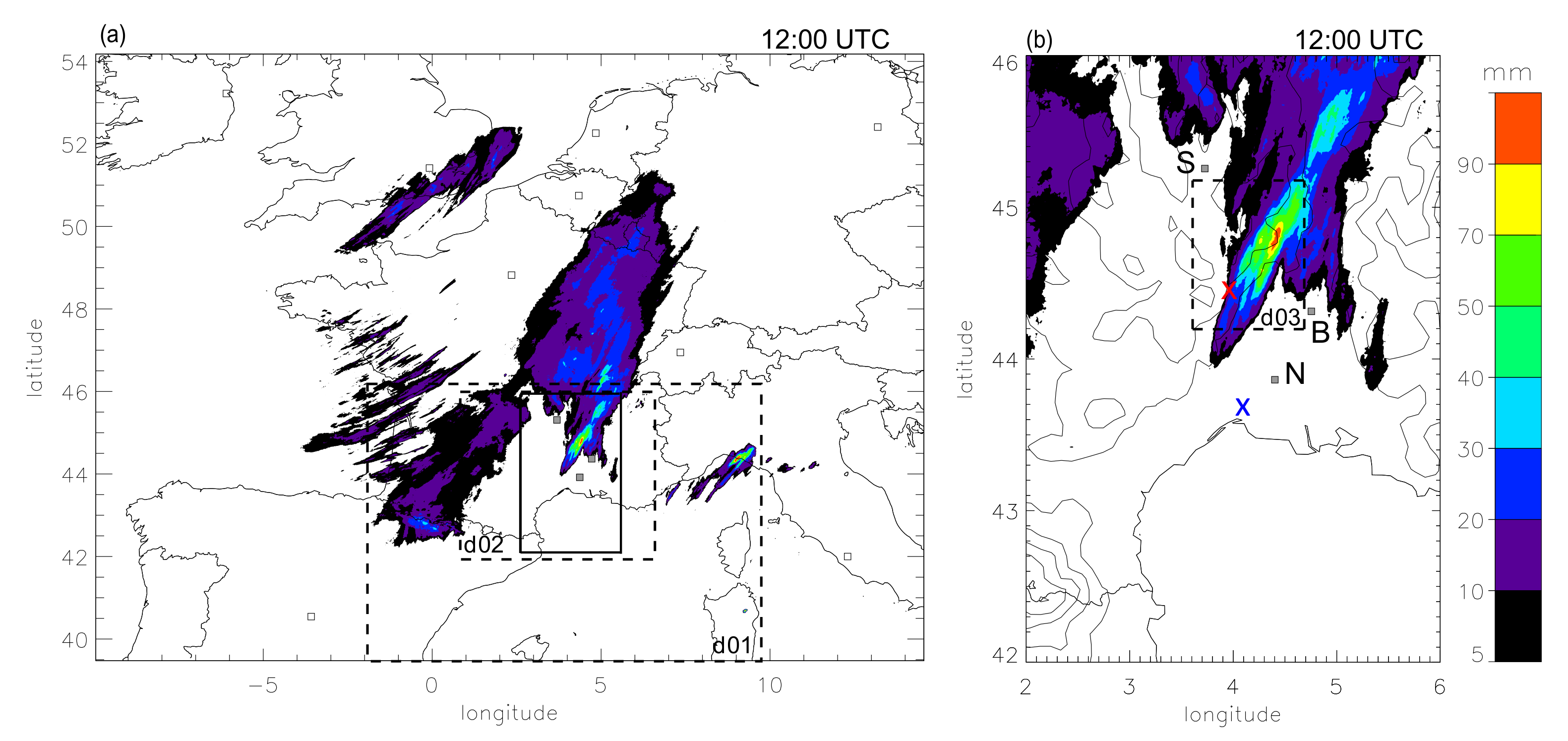
2.1. The HyMeX-IOP7a (26 September 2012, Southern France)
2.2. The DESCAM and WRF Models
2.3. Simulation Strategy
3. Precipitation Features
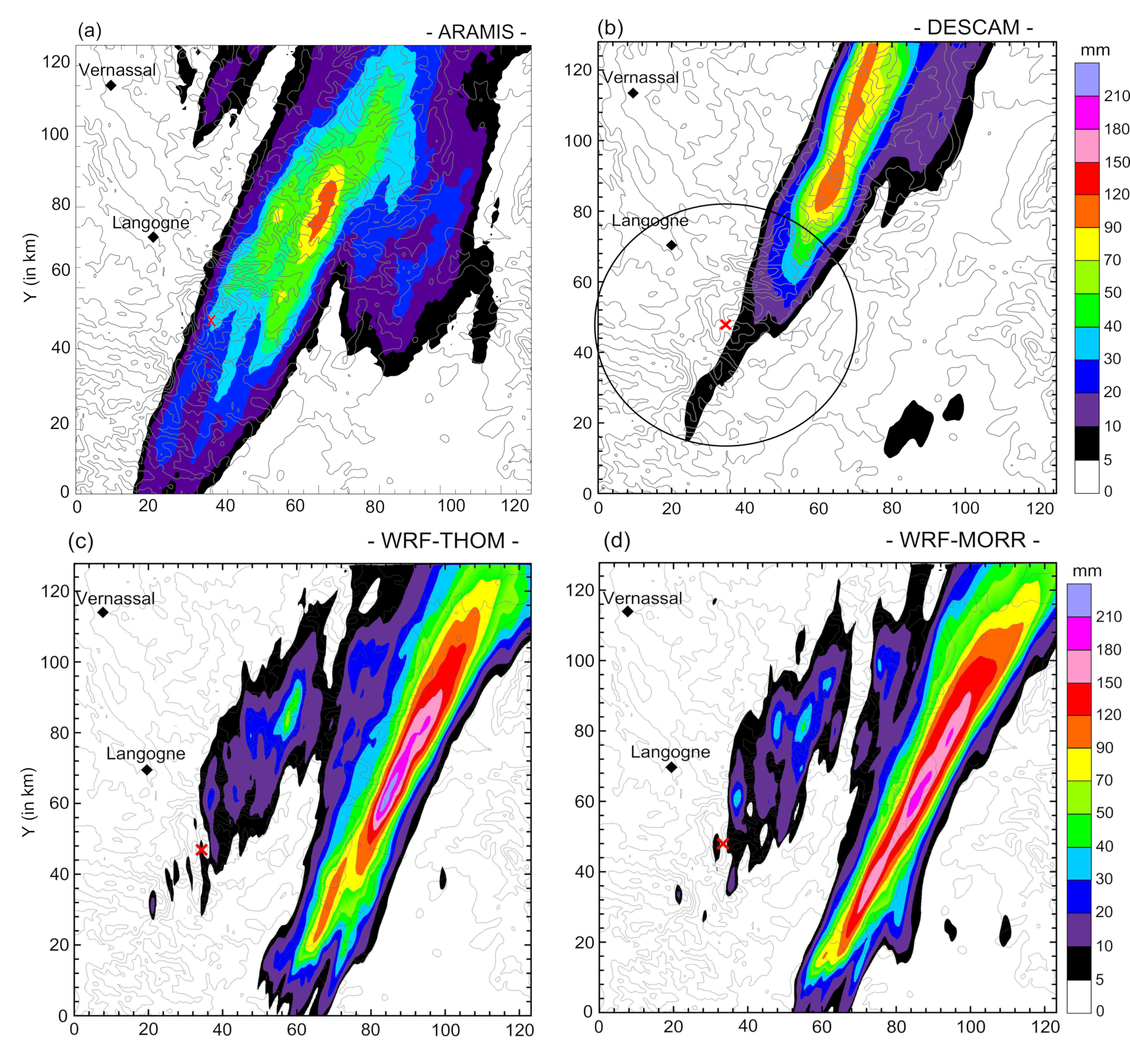
3.1. Accumulated Rain
3.2. Temporal Evolution of the Cumulative Rain
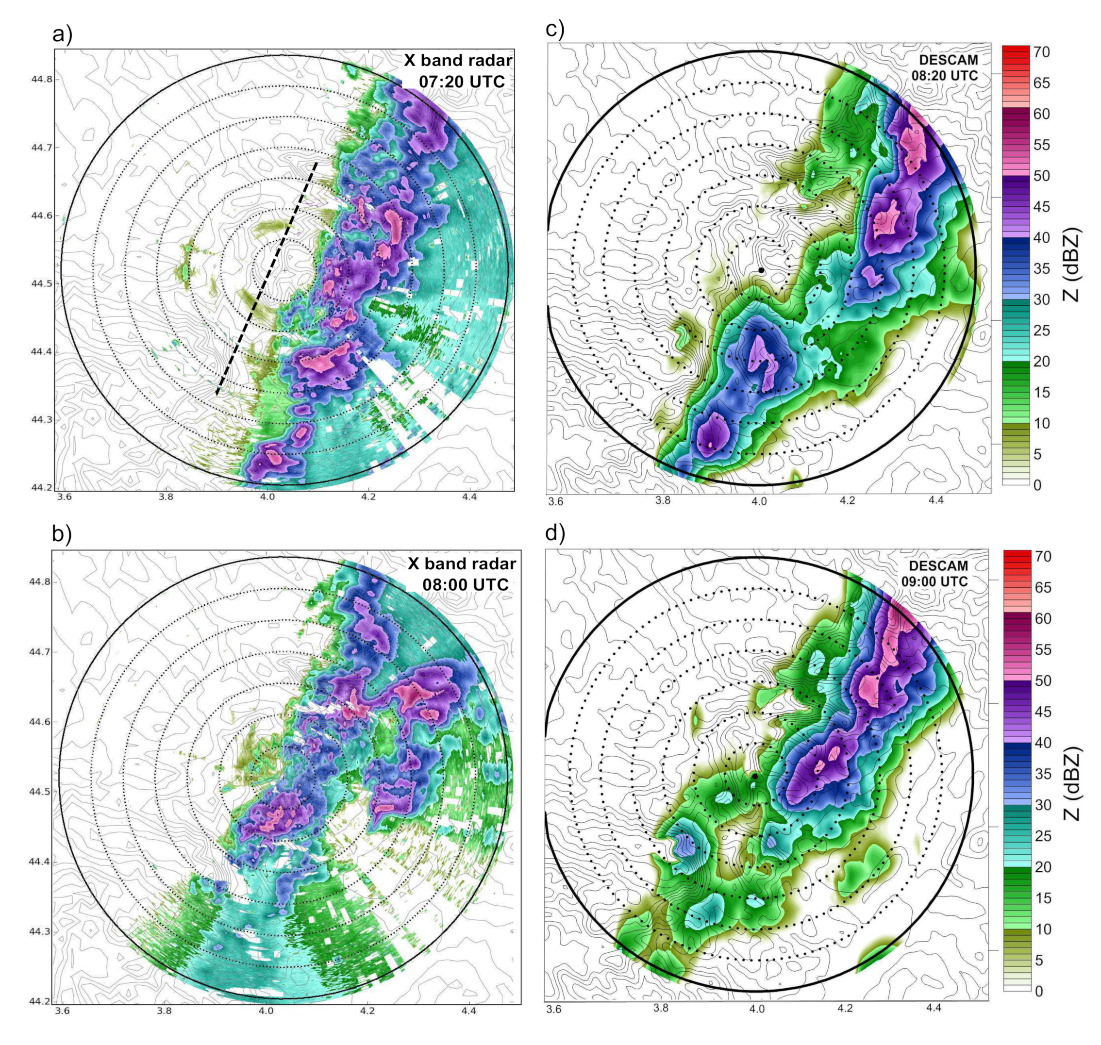
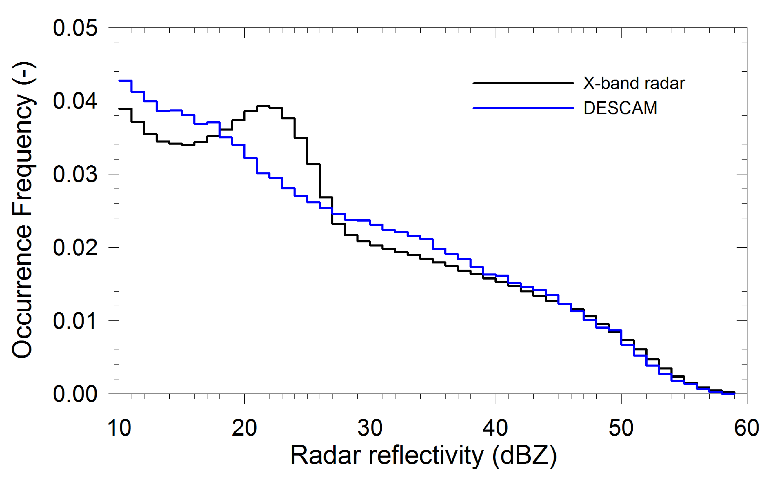
3.3. X-Band Radar Reflectivity Fields
4. Thermodynamics Properties
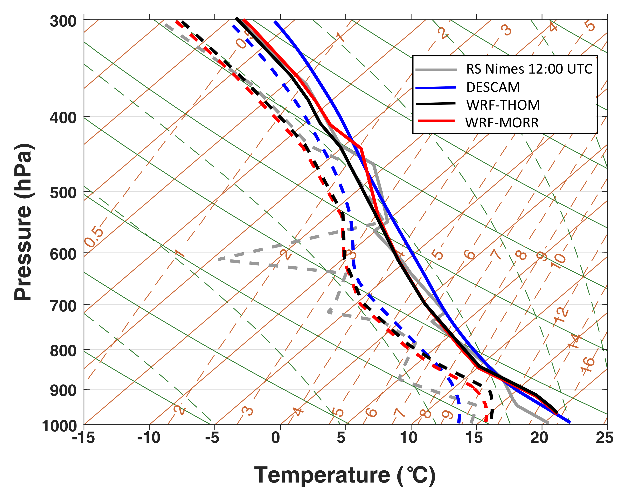
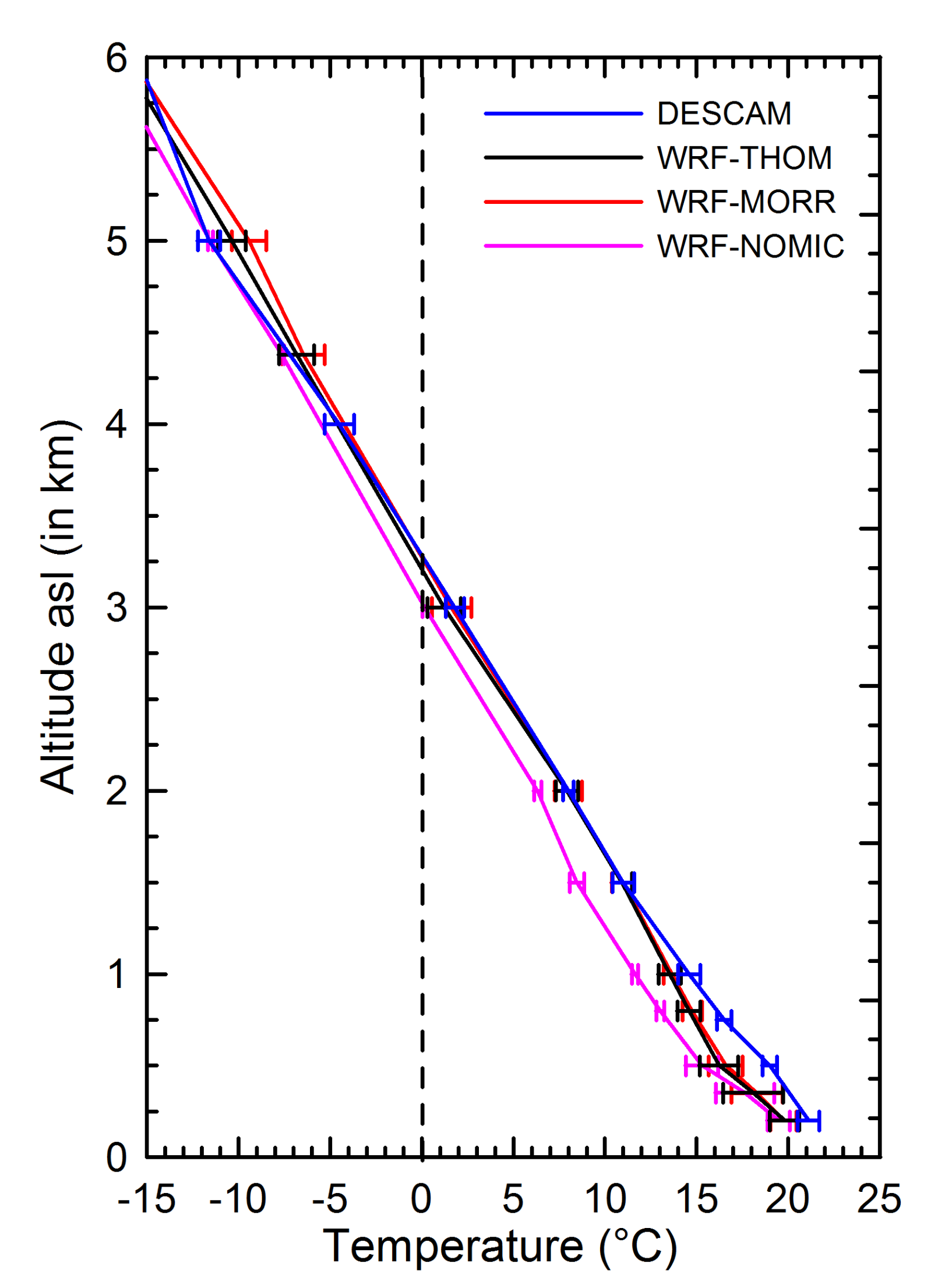
4.1. Temperature and Humidity Profiles
4.2. Impact of the Initial Thermodynamics Fields
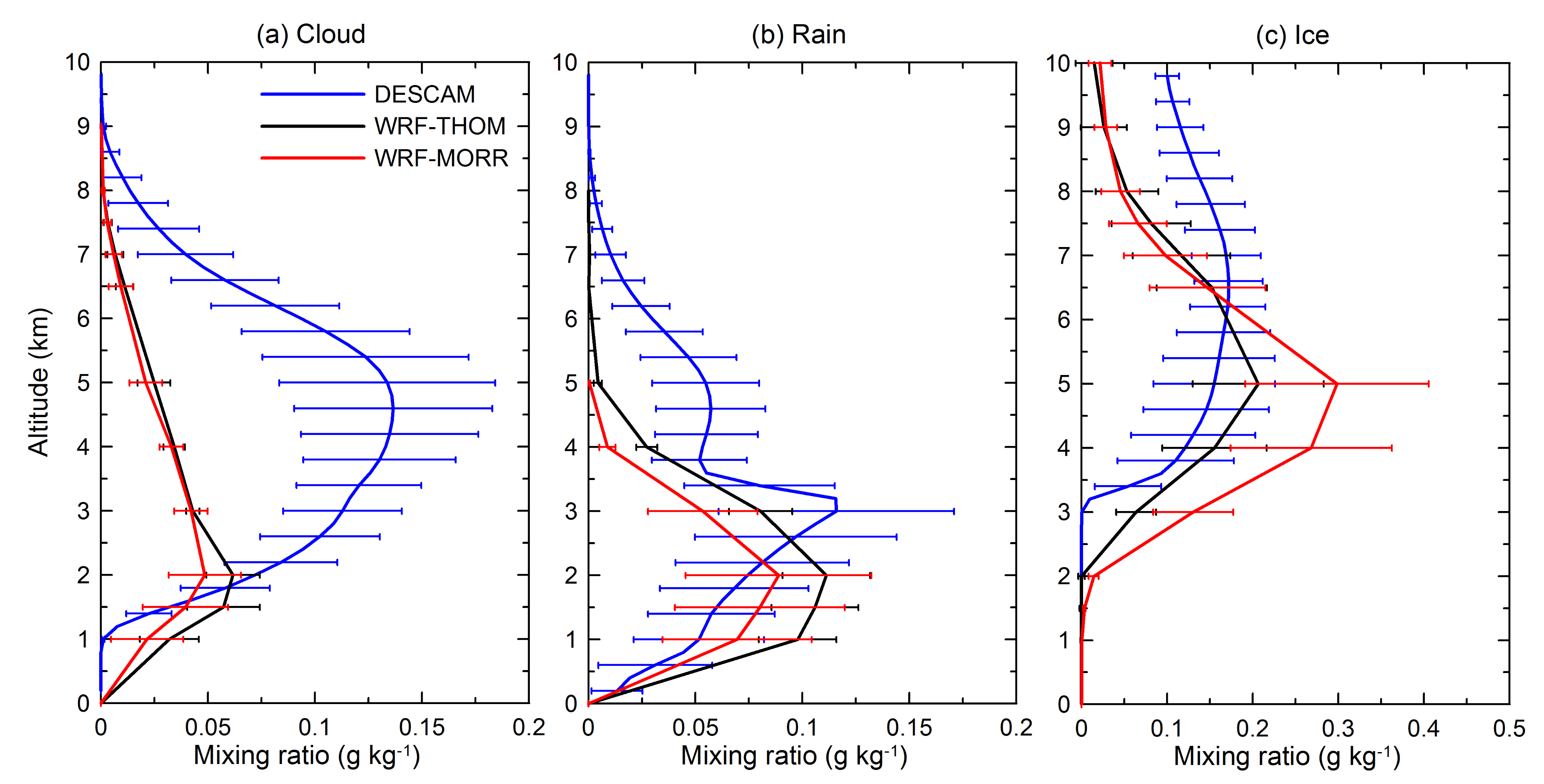
5. Microphysics Features
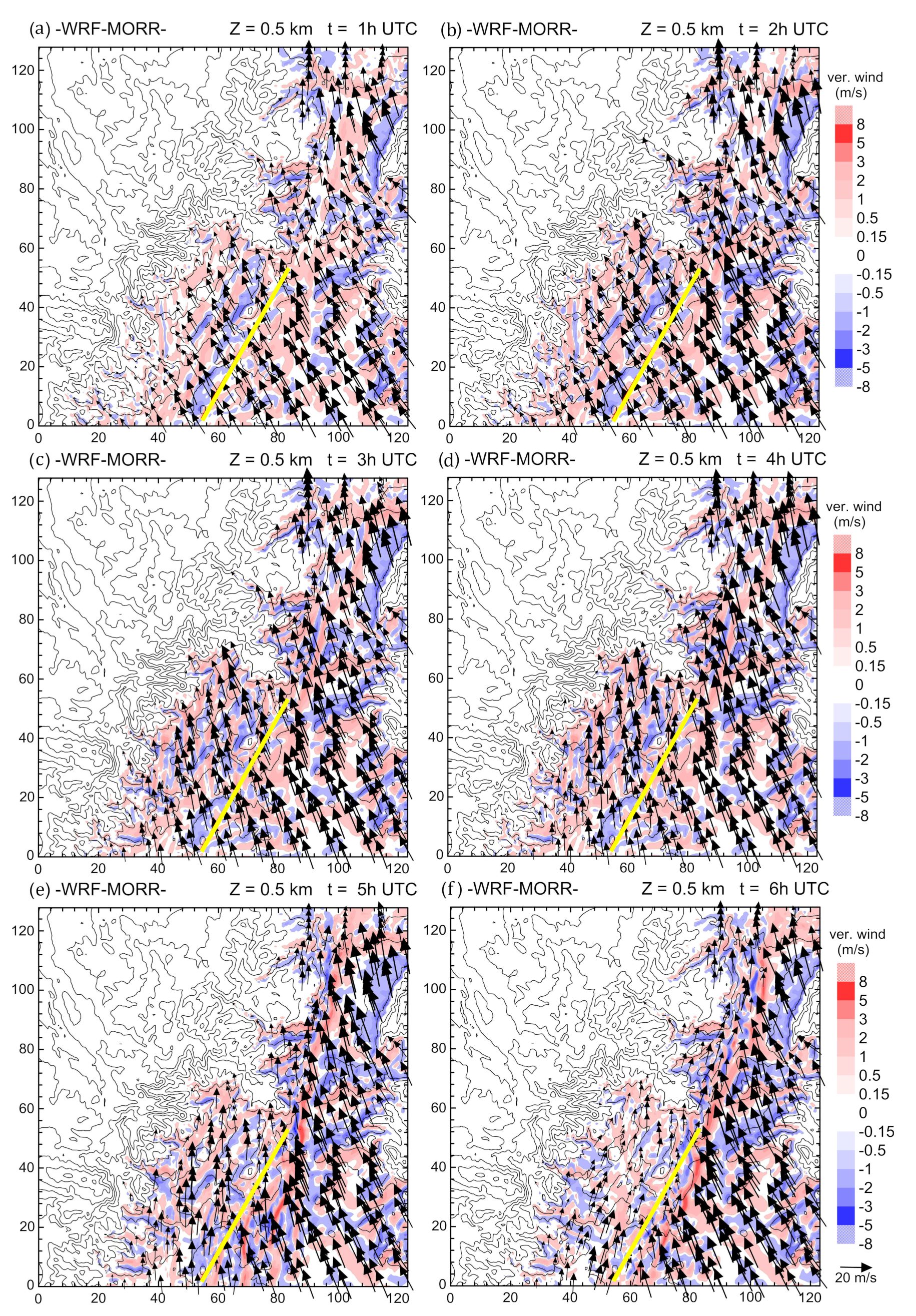
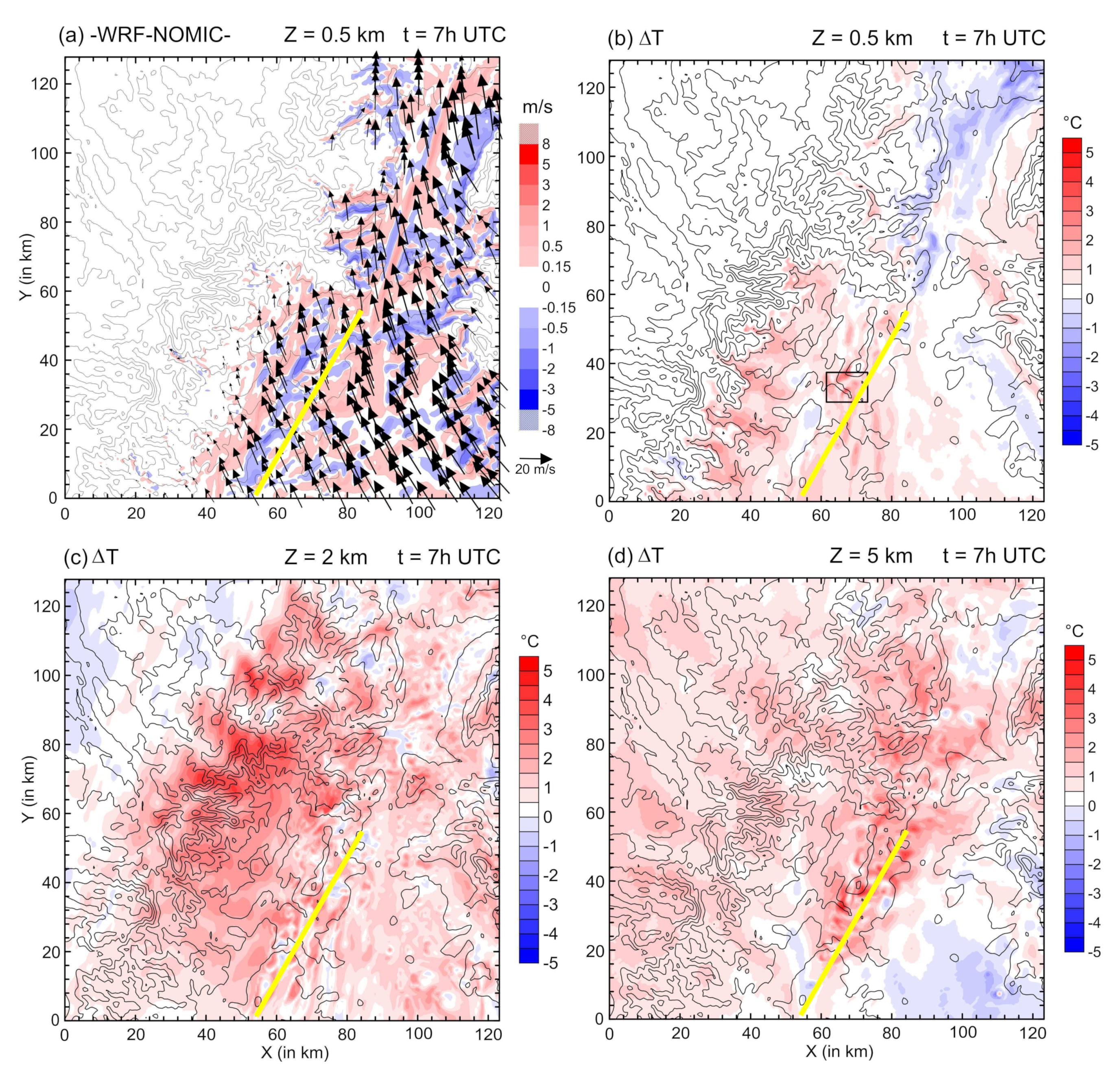
6. Wind Fields
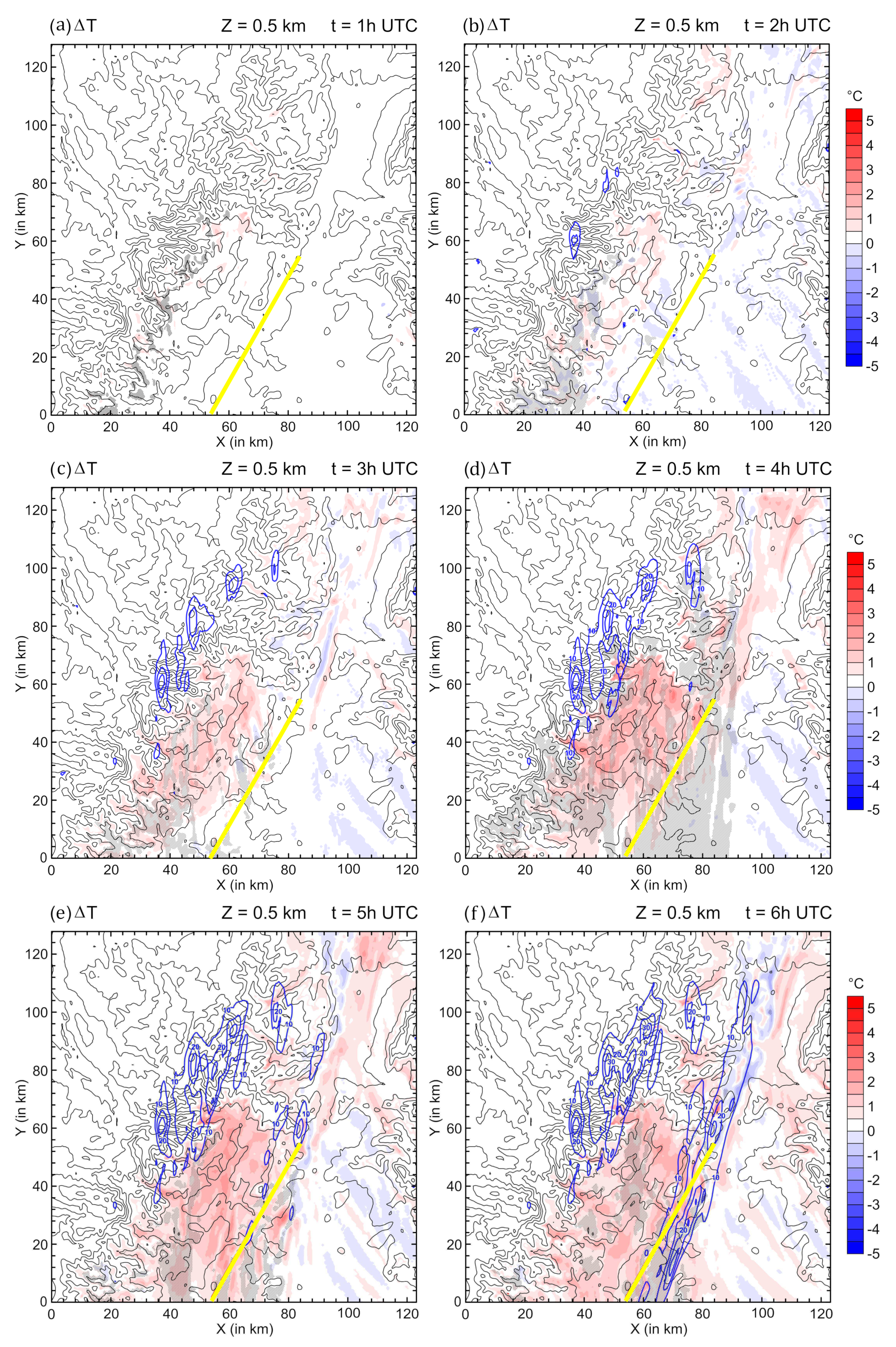
7. Diabatic Effects
8. Conclusions
Author Contributions
Funding
Acknowledgments
Conflicts of Interest
References
- Ricard, D.; Ducrocq, V.; Auger, L. A climatology of the mesoscale environment associated with heavily precipitating events over a northwestern Mediterranean area. J. Appl. Meteor. Climatol. 2012, 51, 468–488. [Google Scholar] [CrossRef]
- Llasat, M.C.; Llasat-Botija, M.; Petrucci, O.; Pasqua, A.A.; Rosselló, J.; Vinet, F.; Boissier, L. Towards a database on societal impact of Mediterranean floods within the framework of the HYMEX project. Nat. Hazard. Earth Syst. 2013, 13, 1337–1350. [Google Scholar] [CrossRef] [Green Version]
- Ducrocq, V.; Nuissier, O.; Ricard, D. A numerical study of three catastrophic precipitating events over Southern France. Part II: Mesoscale trigerring and stationarity factors. Quart. J. R. Meteor. Soc. 2008, 134, 131–145. [Google Scholar] [CrossRef]
- Buzzi, A.; Davolio, S.; Malguzzi, P.; Drofa, O.; Mastrangelo, D. Heavy rainfall episodes over Liguria of autumn 2011: Numerical forecasting experiments. Nat. Hazard. Earth Syst. 2014, 14, 1325–1340. [Google Scholar] [CrossRef] [Green Version]
- Nuissier, O.; Joly, B.; Joly, A.; Ducrocq, V.; Arbogast, P. A statistical downscaling to identify the large-scale circulation patterns associated with heavy precipitation events over southern France. Quart. J. R. Meteor. Soc. 2011, 137, 1812–1827. [Google Scholar] [CrossRef]
- Duffourg, F.; Ducrocq, V. Origin of the moisture feeding the Heavy Precipitating Systems over Southeastern France. Nat. Hazard. Earth Syst. 2011, 11, 1163–1178. [Google Scholar] [CrossRef] [Green Version]
- Bousquet, O.; Smull, B. Observations and impacts of upstream blocking during a widespread orographic precipitating event. Quart. J. Roy. Meteor. Soc. 2003, 129, 391–409. [Google Scholar] [CrossRef]
- Drobinski, P.; Ducrocq, V.; Alpert, P.; Anagnostou, E.; Béranger, K.; Borga, M.; Braud, I.; Chanzy, A.; Davolio, S.; Delrieu, G.; et al. HyMEX: A 10-year multidisciplinary program on the Mediterranean water cycle. Bull. Am. Meteor. Soc. 2014, 95, 1063–1082. [Google Scholar] [CrossRef]
- Ducrocq, V.; Braud, I.; Davolio, S.; Ferretti, R.; Flamant, C.; Jansa, A.; Kalthoff, N.; Richard, E.; Taupier-Letage, I.; Ayral, P.A.; et al. HyMeX-SOP1: The field campaign dedicated to heavy precipitation and flash flooding in the Northwestern Mediterranean. Bull. Am. Meteor. Soc. 2014, 95, 1083–1100. [Google Scholar] [CrossRef]
- Clark, A.J.; Weiss, S.J.; Kain, J.S.; Jirak, I.L.; Coniglio, M.; Melick, C.J.; Siewert, C.; Sobash, R.A.; Marsh, P.T.; Dean, A.R.; et al. An Overview of the 2010 Hazardous Weather Testbed Experimental Forecast Program Spring Experiment. Bull. Am. Meteor. Soc. 2012, 93, 55–74. [Google Scholar] [CrossRef]
- Kanji, Z.A.; Ladino, L.A.; Wex, H.; Boose, Y.; Burkert-Kohn, M.; Cziczo, D.J.; Krämer, M. Overview of ice nucleating particles. Meteor. Monogr. 2017, 58, 1. [Google Scholar] [CrossRef] [Green Version]
- Hiron, T.; Flossmann, A.I. A Study of the Role of the Parameterization of Heterogeneous Ice Nucleation for the Modeling of Microphysics and Precipitation of a Convective Cloud. J. Atmos. Sci. 2015, 72, 3322–3339. [Google Scholar] [CrossRef]
- Pruppacher, H.R.; Klett, J.D. Microphysics of Clouds and Precipitation; Second Revised and Expanded Edition with an Introduction to Cloud Chemistry and Cloud Electricity; Springer: Dordrecht, The Netherlands; Heidelberg/Berlin, Germany; London, UK; New York, NY, USA, 2010; p. 954. [Google Scholar]
- Thompson, G.; Rasmussen, R.M.; Manning, K. Explicit forecasts of winter precipitation using an improved bulk microphysics scheme. Part I: Description and sensitivity analysis. Mon. Weather Rev. 2004, 132, 519–542. [Google Scholar] [CrossRef] [Green Version]
- Planche, C.; Marsham, J.H.; Field, P.R.; Carslaw, K.S.; Hill, A.A.; Mann, G.W.; Shipway, B.J. Precipitation sensitivity to autoconversion rate in a numerical weather-prediction model. Quart. J. R. Meteor. Soc. 2015, 141, 2032–2044. [Google Scholar] [CrossRef] [Green Version]
- McFarquhar, G.M.; Zhang, H.; Heymsfield, G.; Halverson, J.B.; Hood, R.; Dudhia, J.; Marks, F. Factors Affecting the Evolution of Hurricane Erin (2001) and the Distributions of Hydrometeors: Role of Microphysical Processes. J. Atmos. Sci. 2006, 63, 127–150. [Google Scholar] [CrossRef] [Green Version]
- Khain, A.P.; Rosenfeld, D.; Pokrovsky, A. Aerosol impact on the dynamics and microphysics of deep convective clouds. Quart. J. R. Meteor. Soc. 2005, 131, 2639–2663. [Google Scholar] [CrossRef] [Green Version]
- Flossmann, A.I.; Wobrock, W. A review of our understanding of the aerosol—Cloud interaction from the perspective of a bin resolved cloud scale modelling. Atmos. Res. 2010, 97, 478–497. [Google Scholar] [CrossRef]
- Thompson, G.; Field, P.R.; Rasmussen, R.M.; Hall, W.D. Explicit forecasts of winter precipitation using an improved bulk microphysics scheme. Part II: Implementation of a new snow parameterization. Mon. Weather Rev. 2008, 136, 5095–5115. [Google Scholar] [CrossRef]
- Morrison, H.; Thompson, G.; Tatarskii, V. Impact of cloud microphysics on the development of trailing stratiform precipitation in a simulated squall line: Comparison of one- and two-moment schemes. Mon. Weather Rev. 2009, 137, 991–1007. [Google Scholar] [CrossRef] [Green Version]
- Vié, B.; Pinty, J.P.; Berthet, S.; Leriche, M. LIMA (v1.0): A quasi two-moment microphysical scheme driven by a multimodal population of cloud condensation and ice freezing nuclei. Geosci. Model Dev. 2016, 9, 567–586. [Google Scholar] [CrossRef] [Green Version]
- Kessler, E. On the distribution and continuity of water substance in atmospheric situations. Meteorol. Monogr. 1969, 32, 1–84. [Google Scholar]
- Cohard, J.M.; Pinty, J.P. A comprehensive two-moment warm microphysical bulk scheme. I: Description and tests. Quart. J. R. Meteor. Soc. 2000, 126, 1815–1842. [Google Scholar] [CrossRef]
- Khairoutdinov, M.; Kogan, Y. A New Cloud Physics Parameterization in a Large-Eddy Simulation Model of Marine Stratocumulus. Mon. Weather Rev. 2000, 128, 229–243. [Google Scholar] [CrossRef]
- Morrison, H.; Milbrandt, J.A. Parameterization of ice microphysics based on the prediction of bulk particle properties. Part I: Scheme description and idealized tests. J. Atmos. Sci. 2015, 72, 287–311. [Google Scholar] [CrossRef]
- Milbrandt, J.A.; Morrison, H. Parameterization of ice microphysics based on the prediction of bulk particle properties. Part III: Introduction of Multiple Free Categories. J. Atmos. Sci. 2016, 73, 975–995. [Google Scholar] [CrossRef]
- Pinty, J.P.; Jabouille, P. A mixed-phase cloud parameterization for use in a mesoscale non hydrostatic model: Simulations of a squall line and of orographic precipitation. In Proceedings of the Conference on Cloud Physics, Everett, DC, USA, 17–21 August 1998; pp. 217–220. [Google Scholar]
- Wilson, D.R.; Ballard, S.P. A microphysically based precipitation scheme for the UK Meteorological Office Unified Model. Quart. J. R. Meteor. Soc. 1999, 125, 1607–1633. [Google Scholar] [CrossRef]
- Kagkara, C.; Wobrock, W.; Planche, C.; Flossmann, A. The sensitivity of intense rainfall to aerosol particle loading—A comparison of bin-resolved microphysics modeling with observations of heavy precipitation from HyMeX IOP7a. Nat. Hazards Earth Syst. Sci. 2020, 20, 1469–1483. [Google Scholar] [CrossRef]
- Hally, A.; Richard, E.; Ducrocq, V. An ensemble study of HyMeX IOP6 and IOP7a: Sensitivity to physical and initial and boundary condition uncertainties. Nat. Hazards Earth Syst. Sci. 2014, 14, 1071–1084. [Google Scholar] [CrossRef] [Green Version]
- Tabary, P. The new French operational radar rainfall product. Part I: Methodology. Weather Forecast. 2007, 22, 393–408. [Google Scholar] [CrossRef]
- Planche, C.; Wobrock, W.; Flossmann, A.I.; Tridon, F.; VanBaelen, J.; Pointin, Y.; Hagen, M. The influence of aerosol particle number and hygroscopicity on the evolution of convective cloud systems and their precipitation: A numerical study based on the COPS observations on 12 August 2007. Atmos. Res. 2010, 98, 40–56. [Google Scholar] [CrossRef] [Green Version]
- Clark, T.L.; Hall, W.D.; Coen, J.L. Source Code Documentation for the Clark-Hall Cloud-Scale Model Code Version G3CH01; NCAR Tech. Note NCAR/TN-426+STR; NCAR: Boulder, CO, USA, 1996; p. 182. [Google Scholar]
- Clark, T.L. Block-iterative method of solving the non-hydrostatic pressure in terrain-following coordinates: Two-level pressure and truncation error analysis. J. Appl. Meteor. 2003, 42, 970–983. [Google Scholar] [CrossRef]
- Coen, J.L. Modeling Wildland Fires: A Description of the Coupled Atmosphere-Wildland Fire environment model (CAWFE); NCAR Tech. Note NCAR/TN-500+STR; NCAR: Boulder, CO, USA, 2013; p. 38. [Google Scholar]
- Planche, C.; Wobrock, W.; Flossmann, A.I. The continuous melting process in a cloud-scale model using a bin microphysics scheme. Quart. J. R. Meteor. Soc. 2014, 140, 1986–1996. [Google Scholar] [CrossRef]
- Skamarock, W.C.; Klemp, J.B.; Dudhia, J.; Gill, D.O.; Barker, D.M.; Duda, M.G.; Huang, X.Y.; Wang, W.; Powers, J.G. A Description of the Advanced Research WRF Version 3; NCAR Tech. Note NCAR/TN-475+STR; NCAR: Boulder, CO, USA, 2008; p. 125. [Google Scholar]
- Clark, T.L.; Hall, W.D.; Kerre, R.M.; Middleton, D.; Radke, L.; Ralph, F.; Neiman, P. On the origins of aircraft damaging clear-air turbulence during the 9 December 1992 Colorado downslope windstorm: Numerical simulations and comparison with observations. J. Atmos. Sci. 2000, 57, 1105–1131. [Google Scholar] [CrossRef]
- Wobrock, W.; Flossmann, A.I.; Farley, R.D. Comparison of observed and modeled hailstone spectra during a severe storm over the Northern Pyrenean foothills. Mon. Weather Rev. 2003, 67-68, 685–703. [Google Scholar]
- Leroy, D.; Wobrock, W.; Flossmann, A.I. The role of boundary layer aerosol particles for the development of deep convective clouds: A high-resolution 3D model with detailed (bin) microphysics applied to CRYSTAL-FACE. Atmos. Res. 2009, 91, 62–78. [Google Scholar] [CrossRef]
- Clark, T.L. Numerical simulations with a three dimensional cloud model: Lateral boundary condition experiments and multi-cellular severe storm simulations. J. Atmos. Sci. 1979, 36, 2191–2215. [Google Scholar] [CrossRef] [Green Version]
- Danko, D.M. The digital chart of the world. Geoinfo Syst. 1992, 2, 29–36. [Google Scholar]
- Danielson, J.J.; Gesch, D.B. Global Multi-Resolution Terrain Elevation Data 2010 (GMTED2010); U.S. Geo-logical Survey Open-File Report 2011-1073; Earth Resources Observation and Science (EROS) Center: Sioux Falls, SD, USA, 2011; p. 26. [Google Scholar]
- Planche, C.; Wobrock, W.; Flossmann, A.I.; Tridon, F.; Labbouz, L.; VanBaelen, J. Small scale topography influence on the formation of three convective systems observed during COPS over the Vosges Mountains. Meteorol. Z. 2013, 22, 395–411. [Google Scholar] [CrossRef] [Green Version]
- Tewari, M.; Chen, F.; Wang, W.; Dudhia, J.; LeMone, M.A.; Mitchell, K.; Ek, M.; Gayno, G. Implementation and verification of the unified NOAH land surface model in the WRF model. In Proceedings of the 20th Conference on Weather Analysis and Forecasting/16th Conference on Numerical Weather Prediction, Seattle, DC, USA, 12–16 January 2004; pp. 11–15. [Google Scholar]
- Mlawer, E.J.; Taubman, S.J.; Brown, P.D.; Iacono, M.J.; Clough, S.A. Radiative transfer for inhomogeneous atmospheres: RRTM, a validated k-correlated model for the longwave. J. Geophys. Res. 1997, 102, 663–682. [Google Scholar] [CrossRef] [Green Version]
- Hong, S.Y.; Noh, Y.; Dudhia, J. A New Vertical Diffusion Package with an Explicit Treatment of Entrainment Processes. Mon. Weather Rev. 2006, 134, 2318–2341. [Google Scholar] [CrossRef] [Green Version]
- Kain, J.S. The Kain–Fritsch Convective Parameterization: An Update. J. Appl. Meteor. 2004, 43, 170–181. [Google Scholar] [CrossRef] [Green Version]
- Tridon, F.; Planche, C.; Mroz, K.; Banson, S.; Battaglia, A.; Baelen, J.V.; Wobrock, W. On the realism of the rain microphysics representation of a squall line in the WRF model. Part I: Evaluation with multifrequency radar Doppler spectra observations. Mon. Weather Rev. 2019, 147, 2787–2810. [Google Scholar] [CrossRef] [Green Version]
- Planche, C.; Tridon, F.; Banson, S.; Thompson, G.; Monier, M.; Battaglia, A.; Wobrock, W. On the realism of the rain microphysics representation of a squall line in the WRF model. Part II: Sensitivity studies on the rain Drop Size Distributions. Mon. Weather Rev. 2019, 147, 2811–2825. [Google Scholar] [CrossRef] [Green Version]
- Bott, A. A flux method for the numerical solution of the stochastic collection equation. J. Atmos. Sci. 1998, 55, 2284–2293. [Google Scholar] [CrossRef]
- Hall, W.D. A detailed microphysical model within a two-dimensional dynamic framework: Model description and preliminary results. J. Atmos. Sci. 1980, 37, 2486–2506. [Google Scholar] [CrossRef]
- Koop, T.N.H.P.; Luo, B.; Tsias, A.; Peter, T. Water activity as the determinant for homogeneous ice nucleation in aqueous solution. Nature 2000, 406, 611–615. [Google Scholar] [CrossRef]
- Meyers, M.P.; Demott, P.J.; Cotton, W.R. New primary ice nucleation parameterizations in an explicit cloud model. J. Appl. Meteor. 1992, 31, 708–721. [Google Scholar] [CrossRef] [Green Version]
- Dee, D.P.; Uppala, S.M.; Simmons, A.J.; Berrisford, P.; Poli, P.; Kobayashi, S.; Andrae, U.; Balmaseda, M.A.; Balsamo, G.; Bauer, P.; et al. The ERA-Interim reanalysis: Configuration and performance of the data assimilation system. Quart. J. R. Meteor. Soc. 2011, 137, 553–597. [Google Scholar] [CrossRef]
- Tabary, P.; Augros, C.; Champeaux, J.L.; Chèze, J.L.; Faure, D.; Idziorek, D.; Lorandel, R.; Urban, B.; Vogt, V. Le réseau et les produits radars de Météo-France. La Météorologie 2013, 83, 15–27. [Google Scholar] [CrossRef] [Green Version]
- Boudevillain, B.; Delrieu, G.; Galabertier, B.; Bonnifait, L.; Bouilloud, L.; Kirstetter, P.; Mosini, M. The Cevennes-Vivarais Mediterranean Hydrometeorological Observatory database. Water Resour. Res. 2011, 47. [Google Scholar] [CrossRef]
- Marzoug, M.; Amayenc, P. Improved range-profiling algorithm of rainfall rate from a spaceborne radar with path-integrated attenuation constraint. IEEE Trans. Geosc. Remote Sens. 1991, 29, 584–592. [Google Scholar] [CrossRef]
- Delrieu, G.; Hucke, L.; Creutin, J.D. Attenuation in Rain for X- and C-Band Weather Radar Systems: Sensitivity with respect to the Drop Size Distribution. J. Appl. Meteorol. 1999, 38, 57–68. [Google Scholar] [CrossRef]
- Stephens, G.L.; Vane, D.G.; Boain, R.J.; Mace, G.G.; Sassen, K.; Wang, Z.; The CloudSat Science Team. The CloudSat mission and the A-Train: A new dimension of space-based observations of clouds and precipitation. Bull. Am. Meteor. Soc. 2002, 83, 1771–1790. [Google Scholar] [CrossRef] [Green Version]
- Davolio, S.; Volonté, A.; Manzato, A.; Pucillo, A.; Cicogna, A.; Ferrario, M.E. Mechanisms producing different precipitation patterns over north-eastern Italy: Insights from HyMeX-SOP1 and previous events. Q. J. R. Meteorol. Soc. 2016, 142, 188–205. [Google Scholar] [CrossRef] [Green Version]
- Keil, C.; Baur, F.; Bachmann, K.; Rasp, S.; Schneider, L.; Barthlott, C. Relative contribution of soil moisture, boundary-layer and microphysical perturbations on convective predictability in different weather regimes. Q. J. R. Meteorol. Soc. 2019, 145, 3102–3115. [Google Scholar] [CrossRef]
- Flack, D.L.A.; Gray, S.L.; Plant, R.S. A simple ensemble approach for more robust process-based sensitivity analysis of case studies in convection-permitting models. Q. J. R. Meteorol. Soc. 2019, 145, 3089–3101. [Google Scholar] [CrossRef]


| DESCAM | WRF | |
|---|---|---|
| Microphysics | spectral (bin) representation [18,36] | bulk representation [19,20] |
| Aerosol | spectral (bin) representation | not considered |
| Convection | resolved | resolved |
| Turbulence | 1-order turbulence closure | 1.5-order turbulence closure |
| Topography | GTOPO30 data base (resolution: 30’) [42] | GMTED2010 data base (resolution: 30’) [43] |
| Surface | constant heat & moisture fluxes [44] | Unified Noah Land Surface Model [45] |
| DESCAM | WRF-THOM | WRF-MORR | WRF-NOMIC | |
|---|---|---|---|---|
| Dynamics core | Clark model | WRF-ARW | ||
| Microphysics scheme | DESCAM | Thompson scheme | Morrison scheme | No scheme |
| Initiation & Forcing | IFS operational data & every 12 h | |||
| Number of domains | 3 nested domains | |||
| Horizontal resolutions | 8 km, 2 km and 0.5 km | |||
| Vertical resolution | 40–230 m | 60–305 m | ||
| Number of levels | 80 | 72 | ||
| ARAMIS OBS | DESCAM IFS | WRF-THOM IFS | WRF-MORR IFS | WRF-THOM ERA-Interim | WRF-MORR ERA-Interim | |
|---|---|---|---|---|---|---|
| Rain max. (mm/12 h) | 105.3 | 119.5 | 227.7 | 181.7 | 174.1 | 169.2 |
| Mean rain (mm/12 h) | 17.55 | 10.09 | 13.61 | 13.99 | 14.85 | 16.05 |
| Total rain mass (Mt/12 h) | 158.6 | 105.6 | 221.5 | 229.3 | 242.1 | 263.0 |
| Rain area (×103 km2) | 9.04 | 10.78 | 11.93 | 11.98 | 12.82 | 11.54 |
Publisher’s Note: MDPI stays neutral with regard to jurisdictional claims in published maps and institutional affiliations. |
© 2020 by the authors. Licensee MDPI, Basel, Switzerland. This article is an open access article distributed under the terms and conditions of the Creative Commons Attribution (CC BY) license (http://creativecommons.org/licenses/by/4.0/).
Share and Cite
Arteaga, D.; Planche, C.; Kagkara, C.; Wobrock, W.; Banson, S.; Tridon, F.; Flossmann, A. Evaluation of Two Cloud-Resolving Models Using Bin or Bulk Microphysics Representation for the HyMeX-IOP7a Heavy Precipitation Event. Atmosphere 2020, 11, 1177. https://doi.org/10.3390/atmos11111177
Arteaga D, Planche C, Kagkara C, Wobrock W, Banson S, Tridon F, Flossmann A. Evaluation of Two Cloud-Resolving Models Using Bin or Bulk Microphysics Representation for the HyMeX-IOP7a Heavy Precipitation Event. Atmosphere. 2020; 11(11):1177. https://doi.org/10.3390/atmos11111177
Chicago/Turabian StyleArteaga, Diana, Céline Planche, Christina Kagkara, Wolfram Wobrock, Sandra Banson, Frédéric Tridon, and Andrea Flossmann. 2020. "Evaluation of Two Cloud-Resolving Models Using Bin or Bulk Microphysics Representation for the HyMeX-IOP7a Heavy Precipitation Event" Atmosphere 11, no. 11: 1177. https://doi.org/10.3390/atmos11111177