Improving WRF Typhoon Precipitation and Intensity Simulation Using a Surrogate-Based Automatic Parameter Optimization Method


Abstract

1. Introduction
2. Data and Methodology
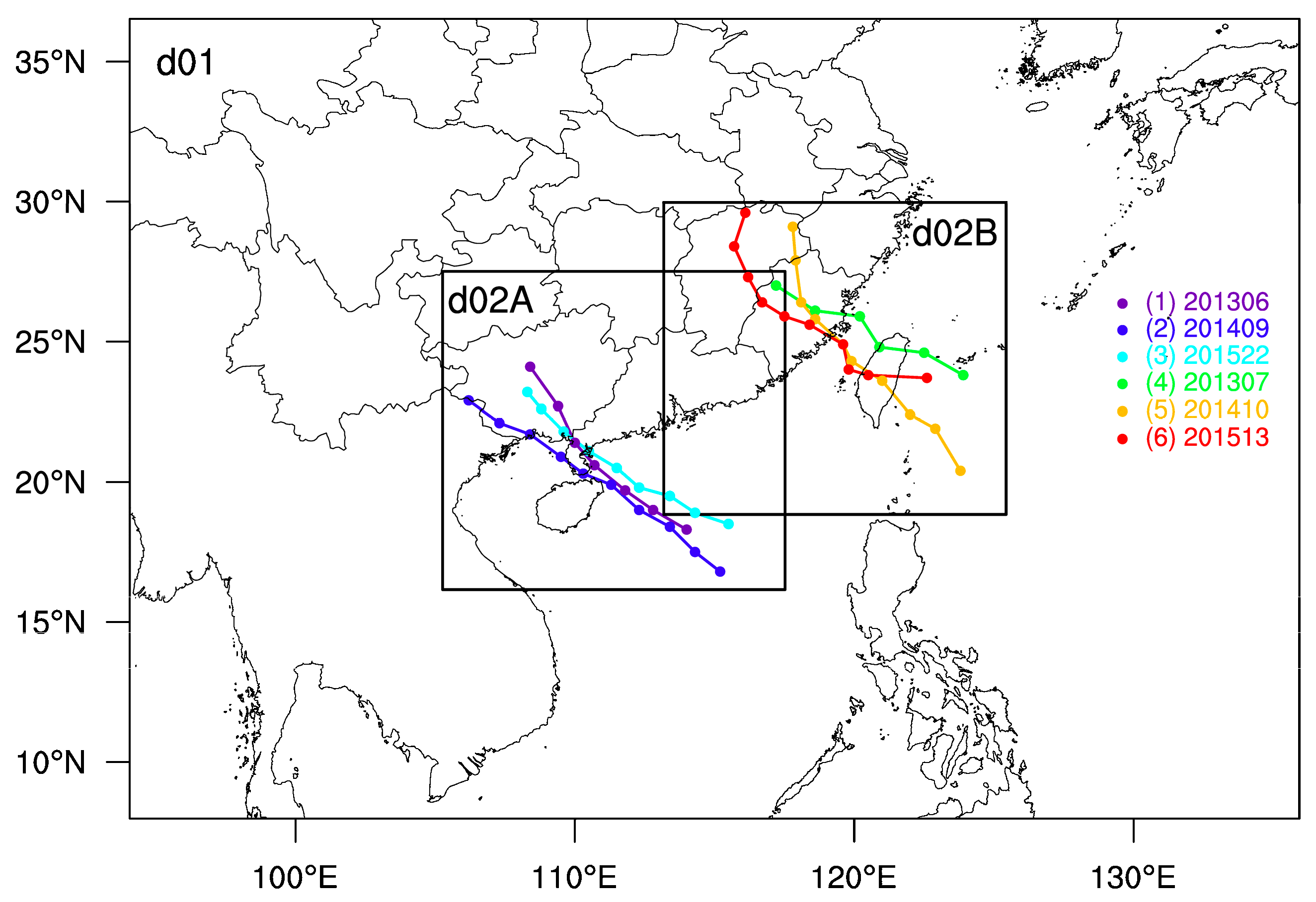
2.1. Observed Data
2.2. WRF Model Configuration for Typhoon Simulations
2.3. Systematic Parameter Optimization Framework
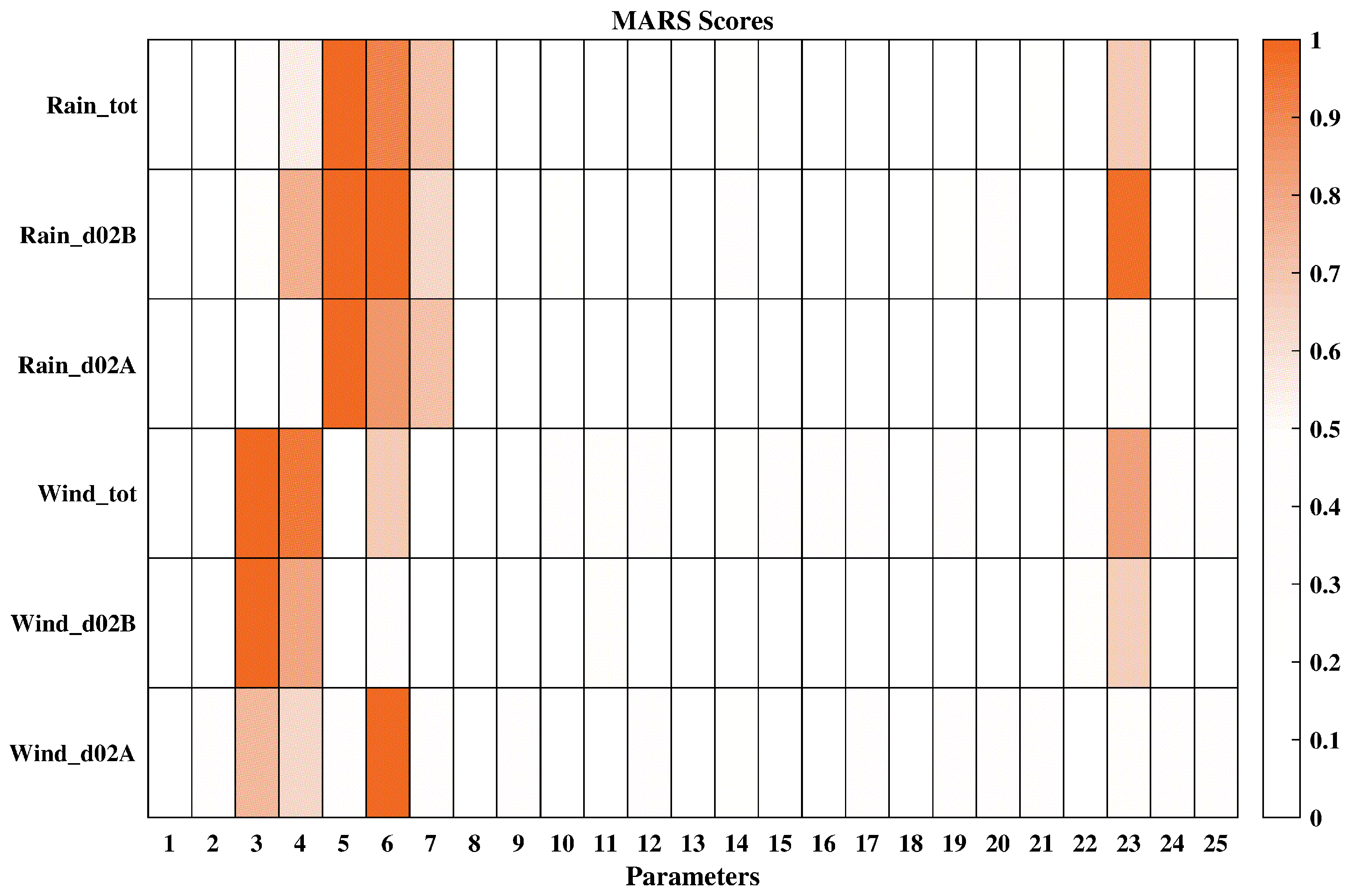
2.3.1. MARS Sensitivity Analysis Method
2.3.2. ASMO Parameter Optimization Method
- Sample to the adjustable parameter ranges using a uniform sampling method. Then these parameter samples are respectively put into the physical model instead of the default parameter values to obtain the corresponding model outputs (or the output errors compared with observed data). The parameter samples and the corresponding model outputs constitute an initial sample set;
- Build a statistical regression model in the initial sample set. Then search for the optimal value of the statistical model using a traditional parameter optimization method. The corresponding optimal parameters (i.e., the optimal parameter values) are finally found;
- Put the optimal parameters of the statistical regression model into the physical model to update the model output. A new sample point is generated based on the optimal parameters and the corresponding physical model output. Update the initial sample point set by adding the new sample point;
- Repeat Steps 2 and 3 until the parameter optimization convergence condition for the physical model is met. The globally optimal parameters of the physical model have now been found.
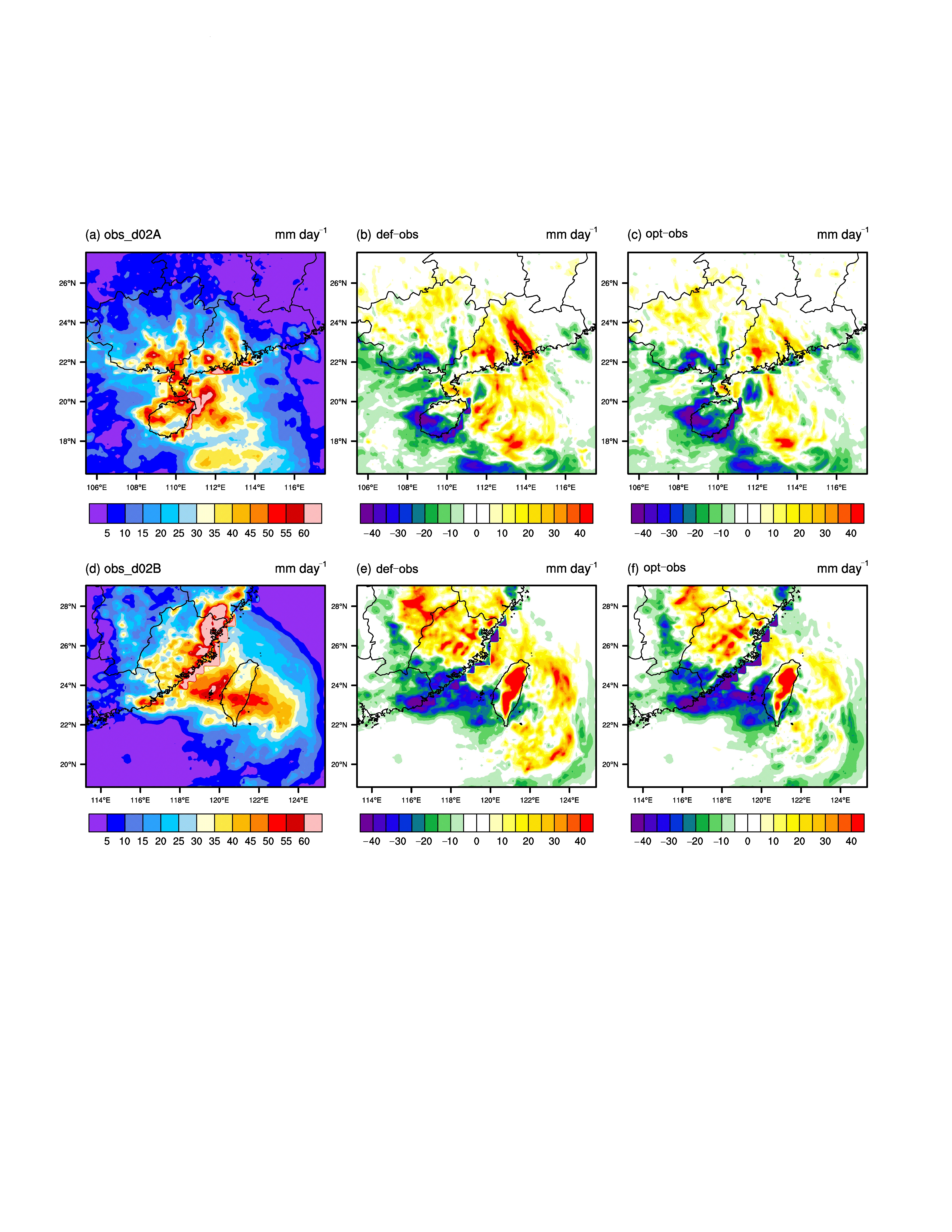
3. Results
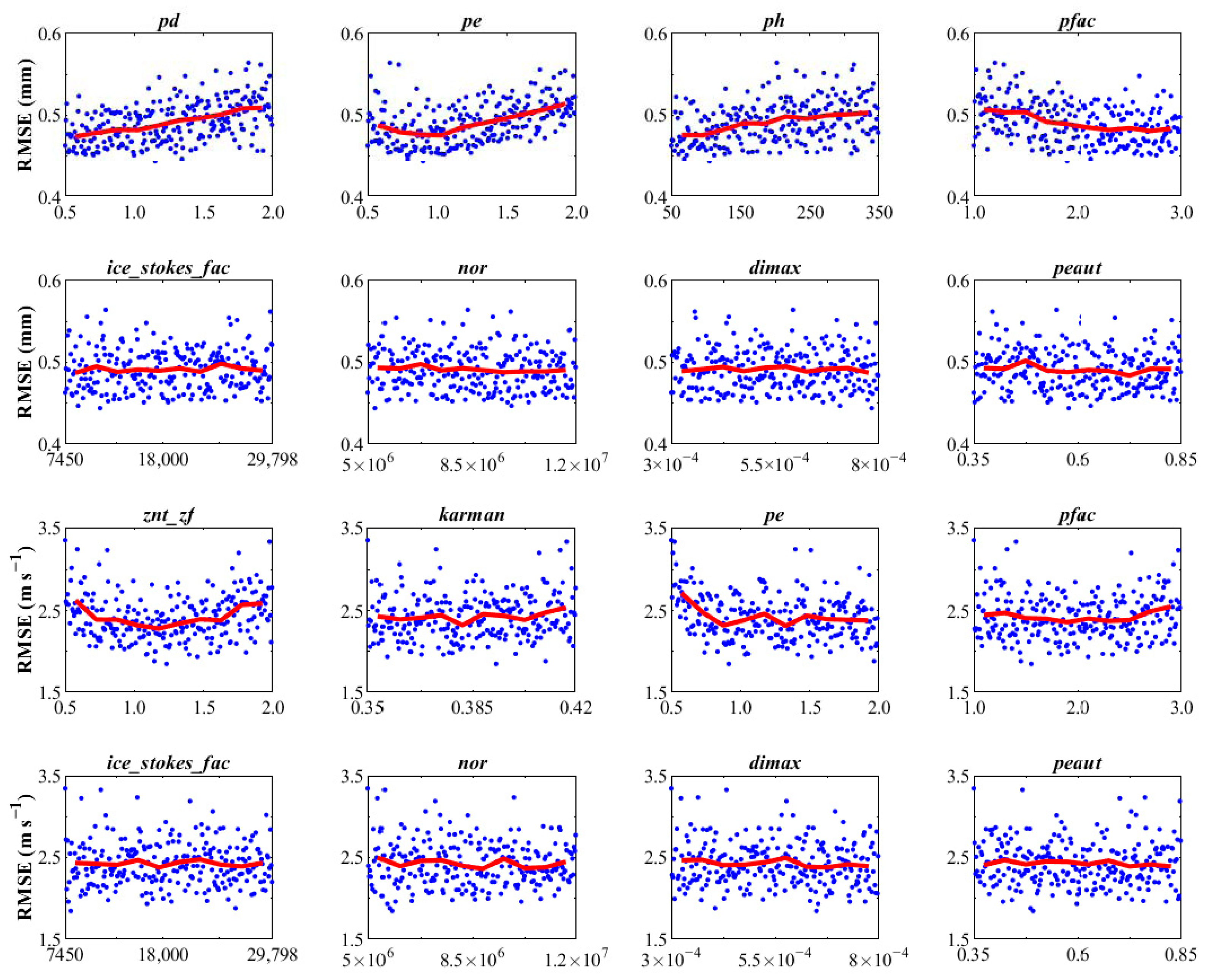
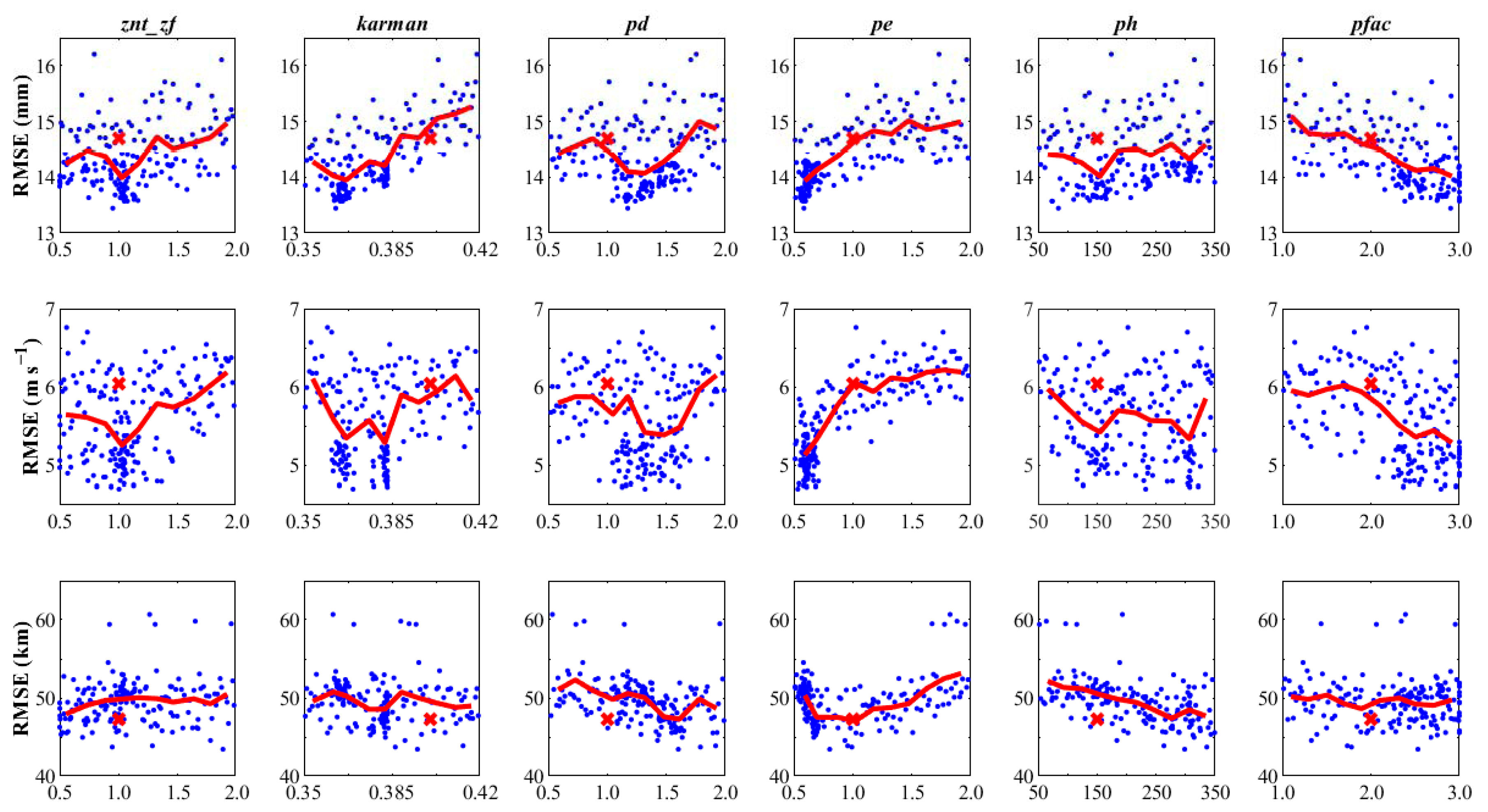
3.1. Sensitivity Analysis Results
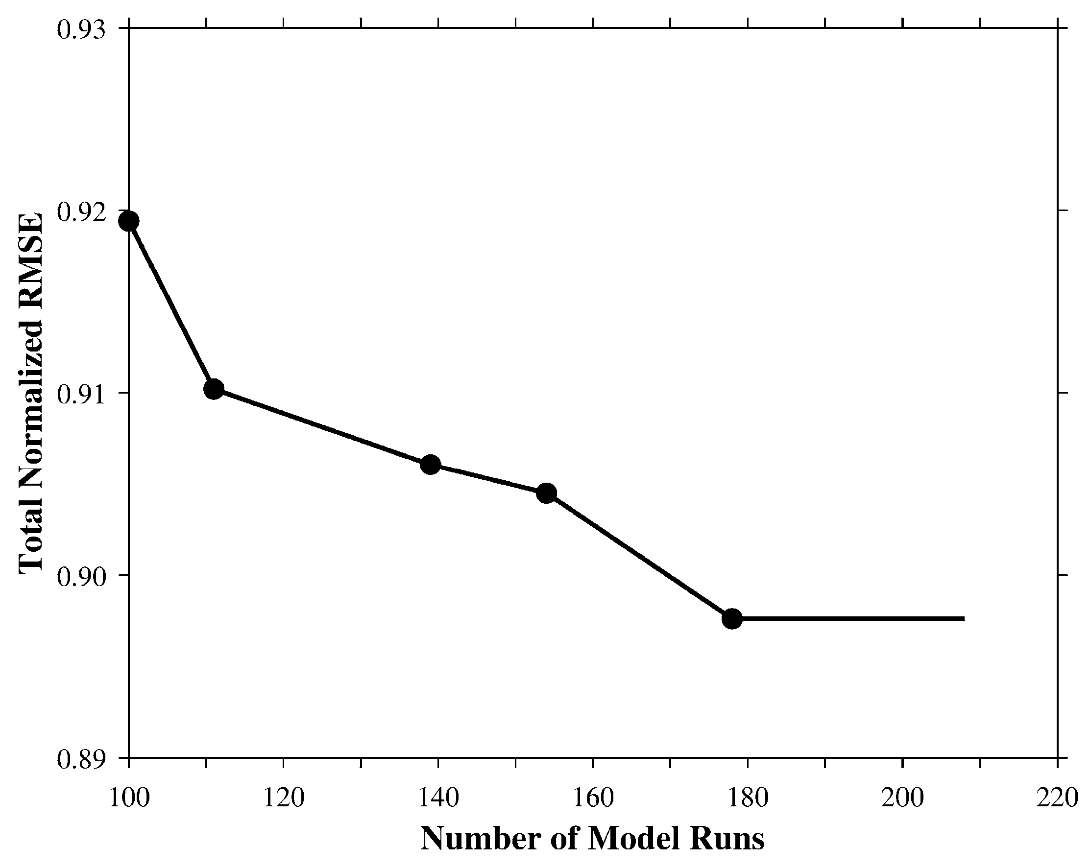
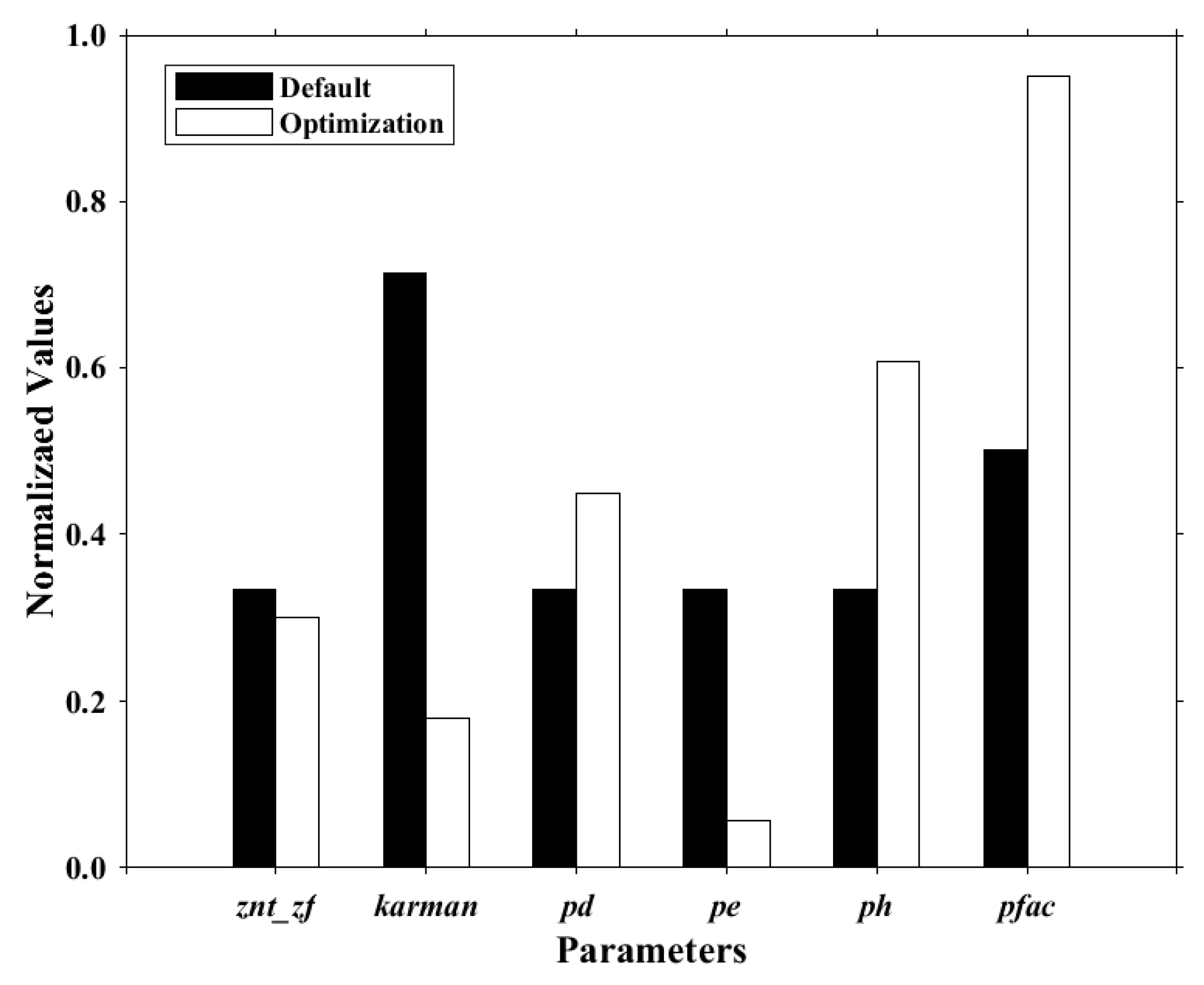
3.2. Parameter Optimization Results
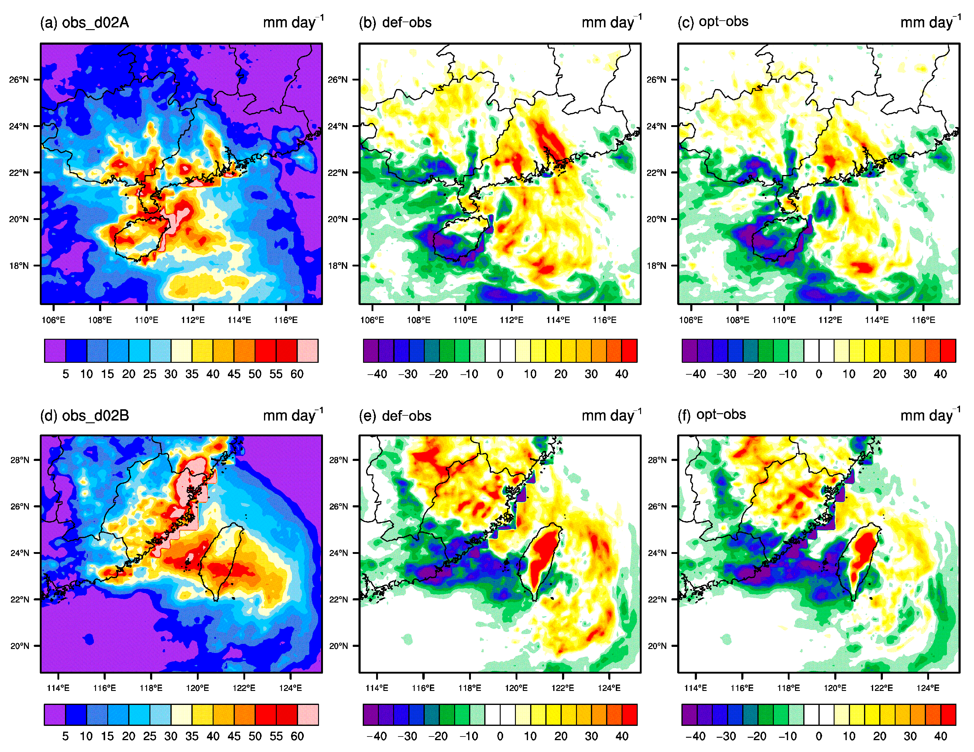
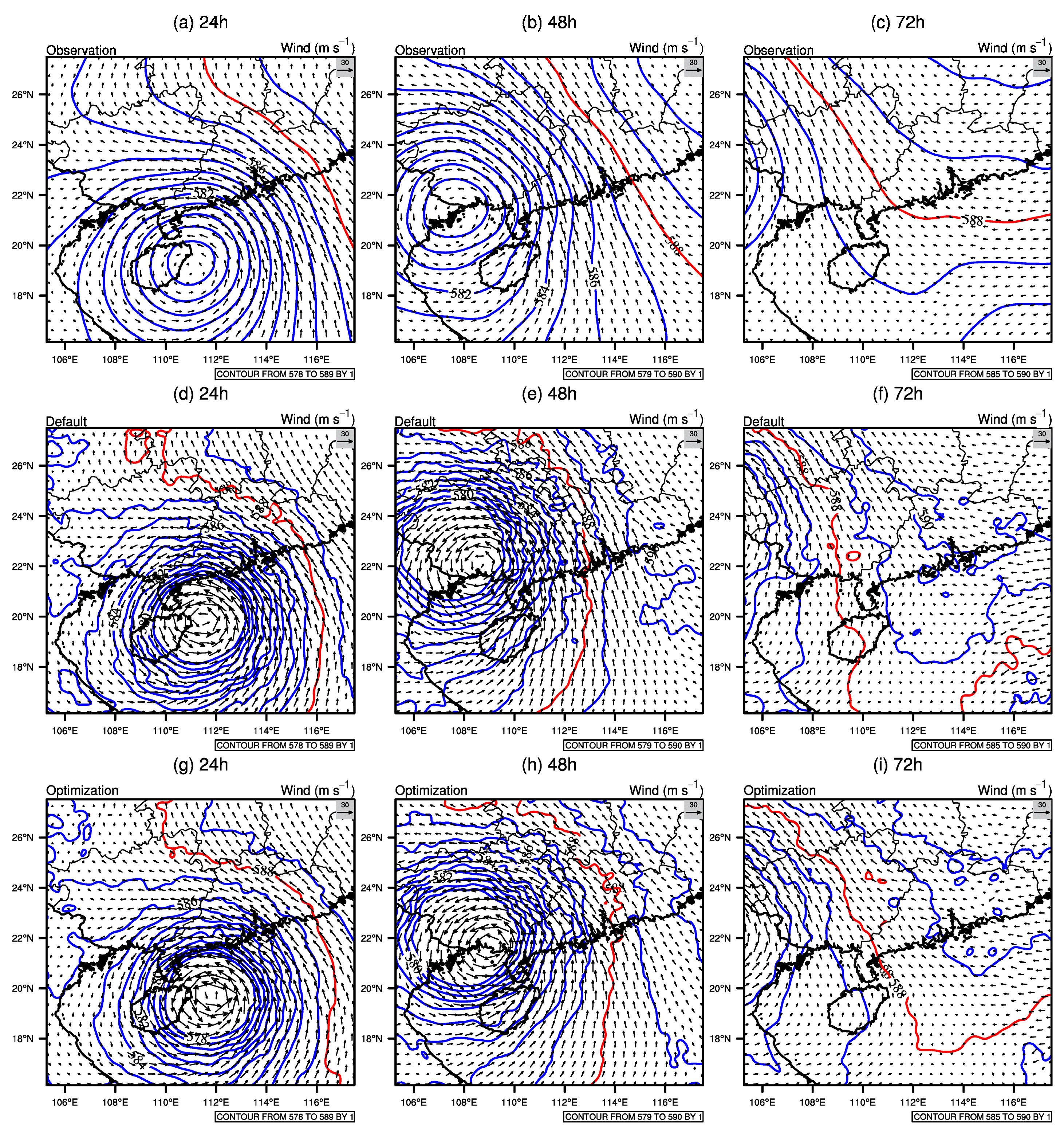
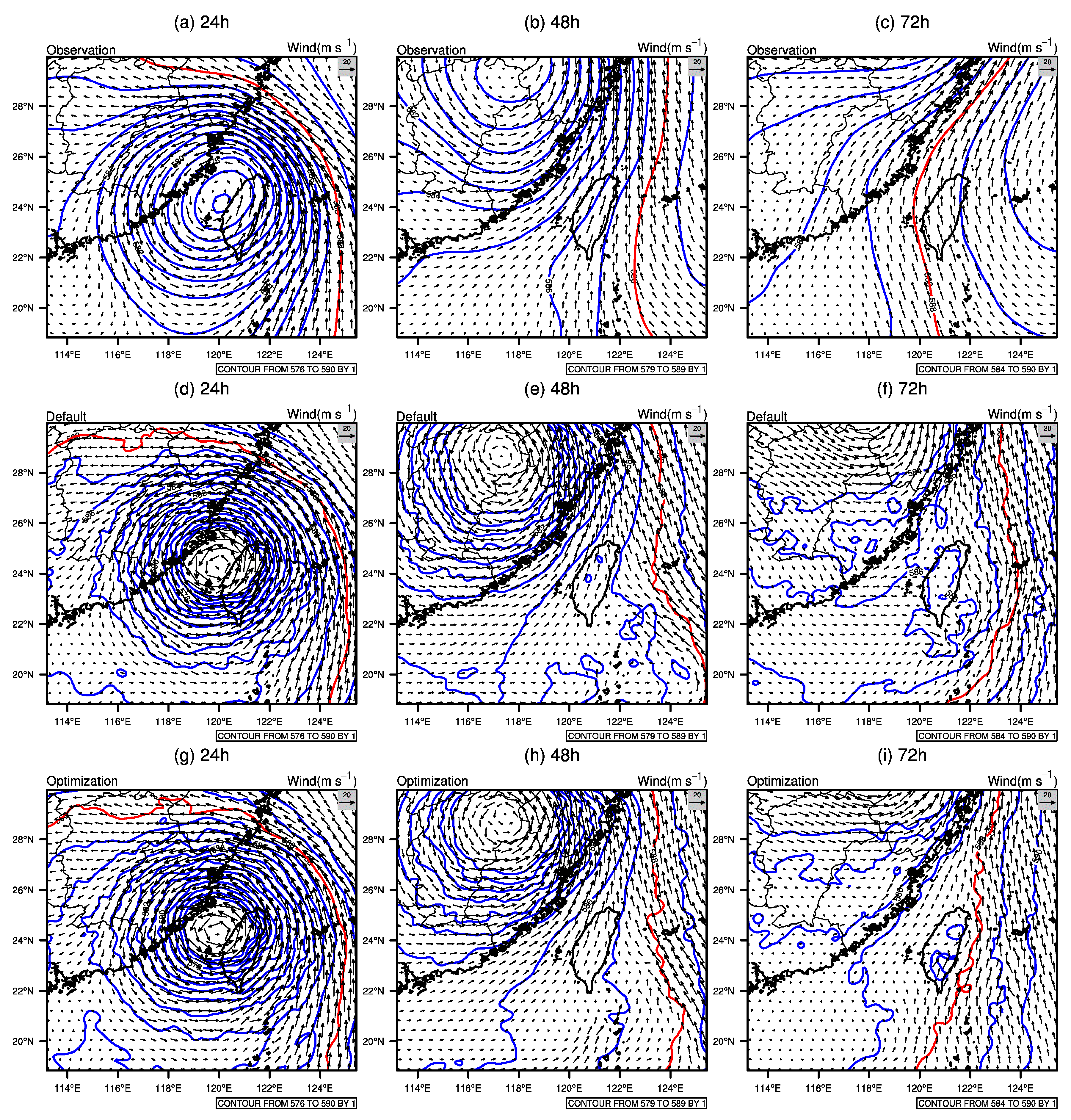
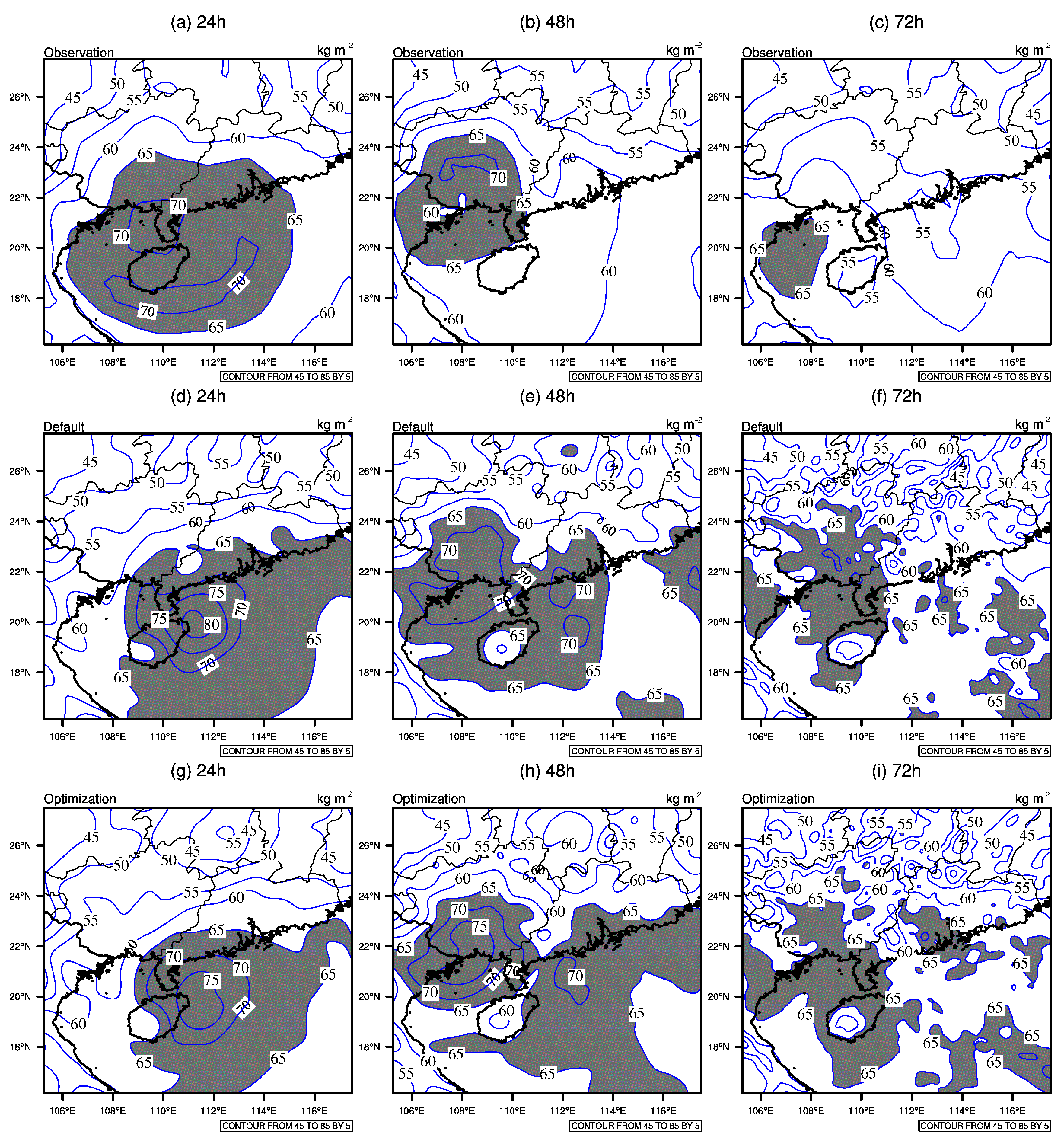
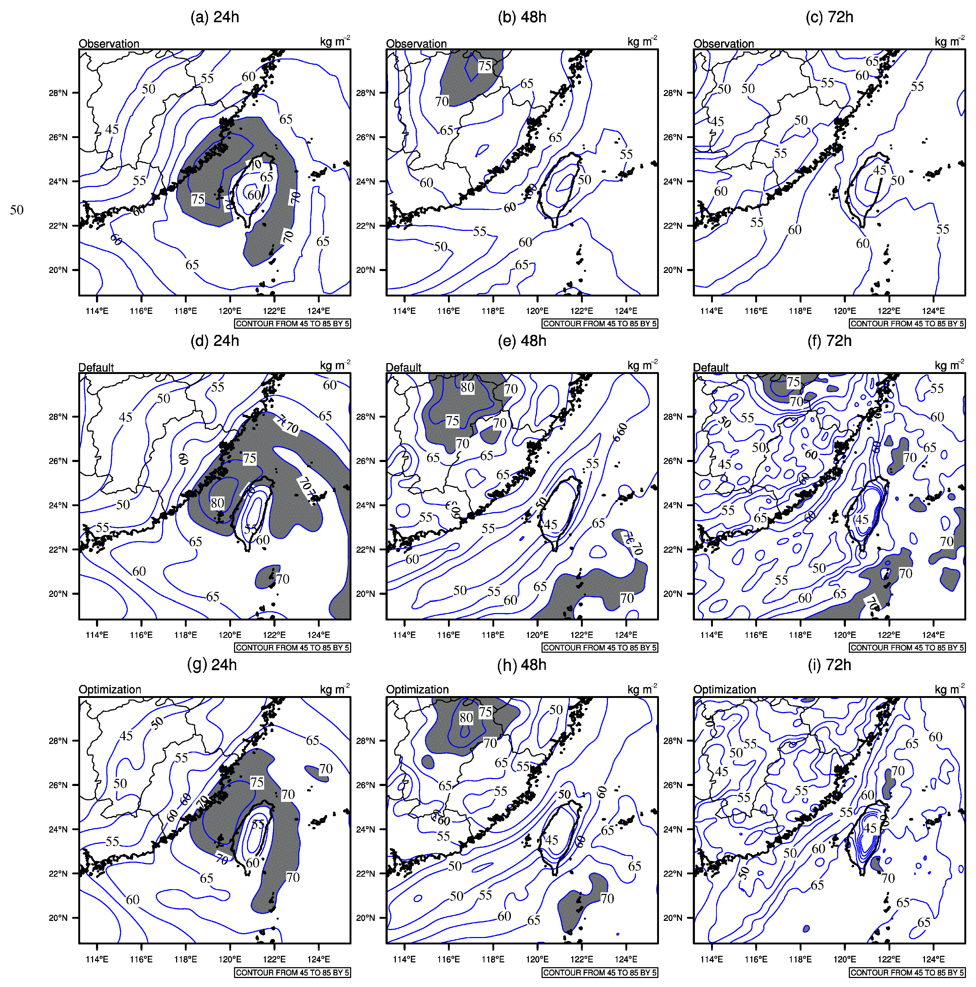
3.3. Atmospheric Structure Analysis
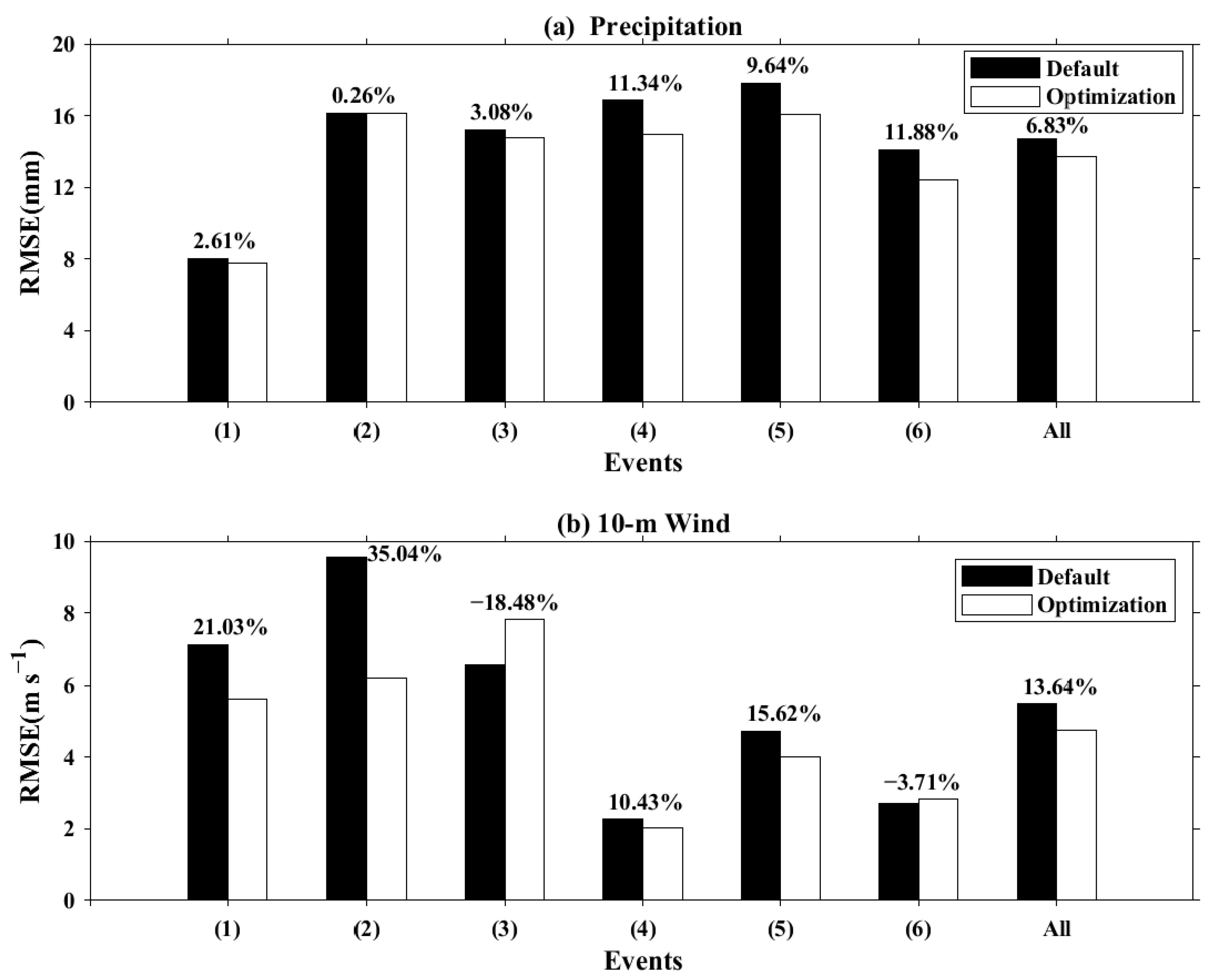
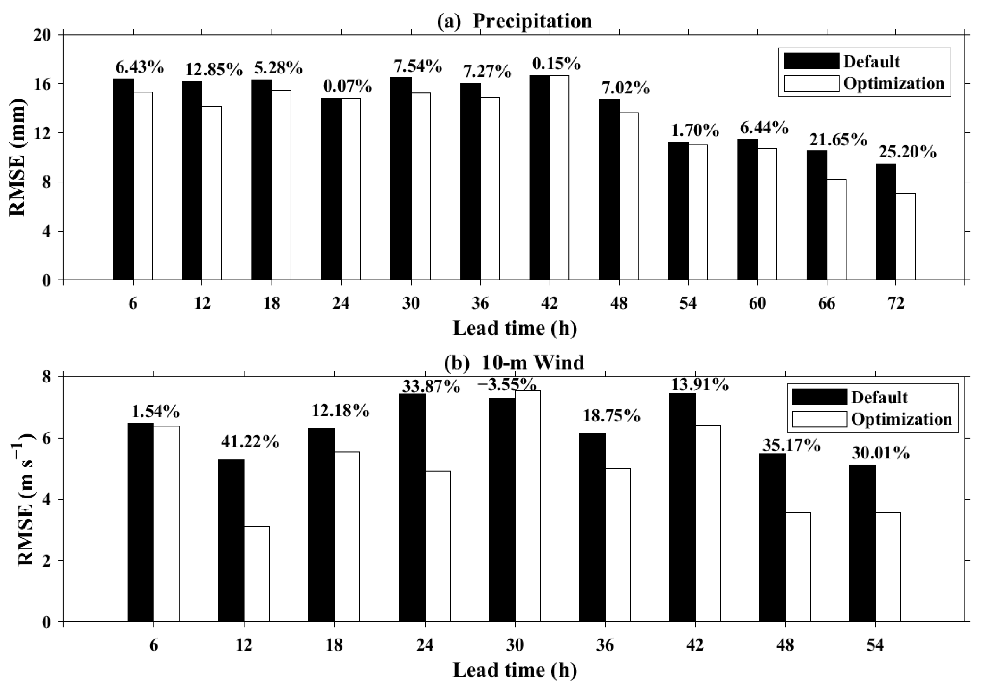
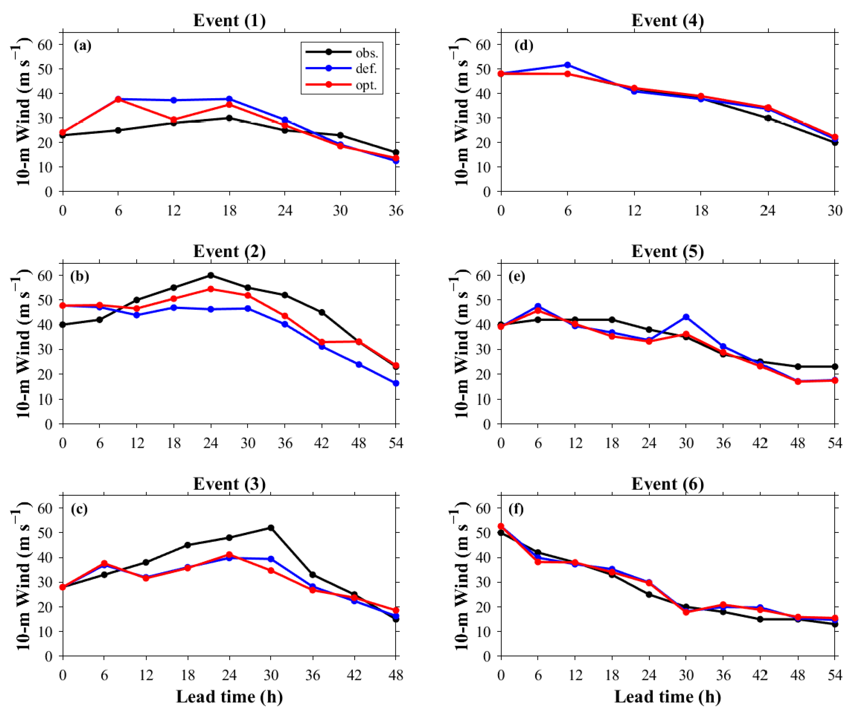
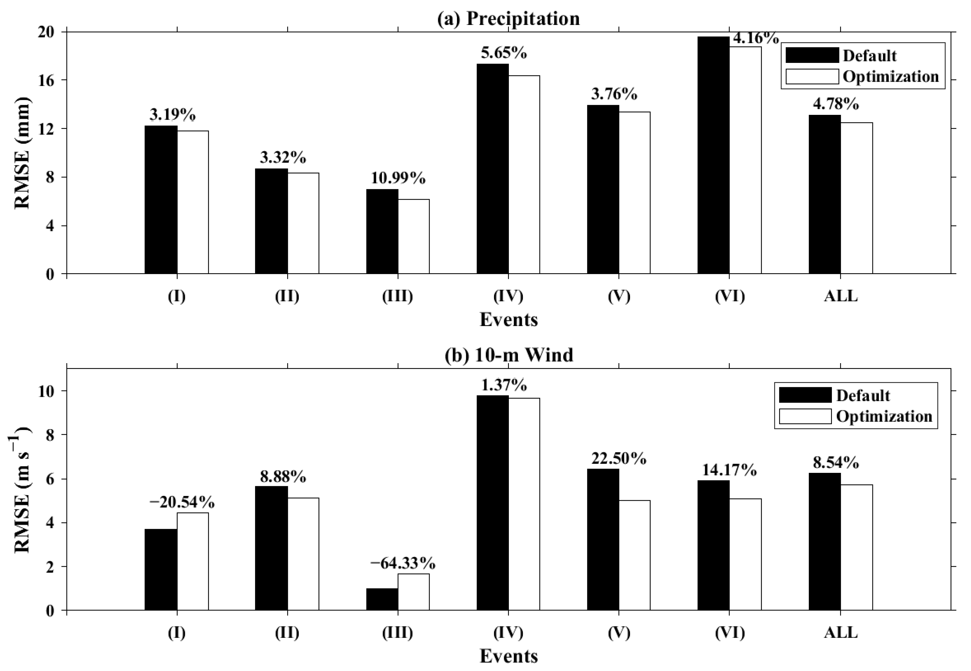
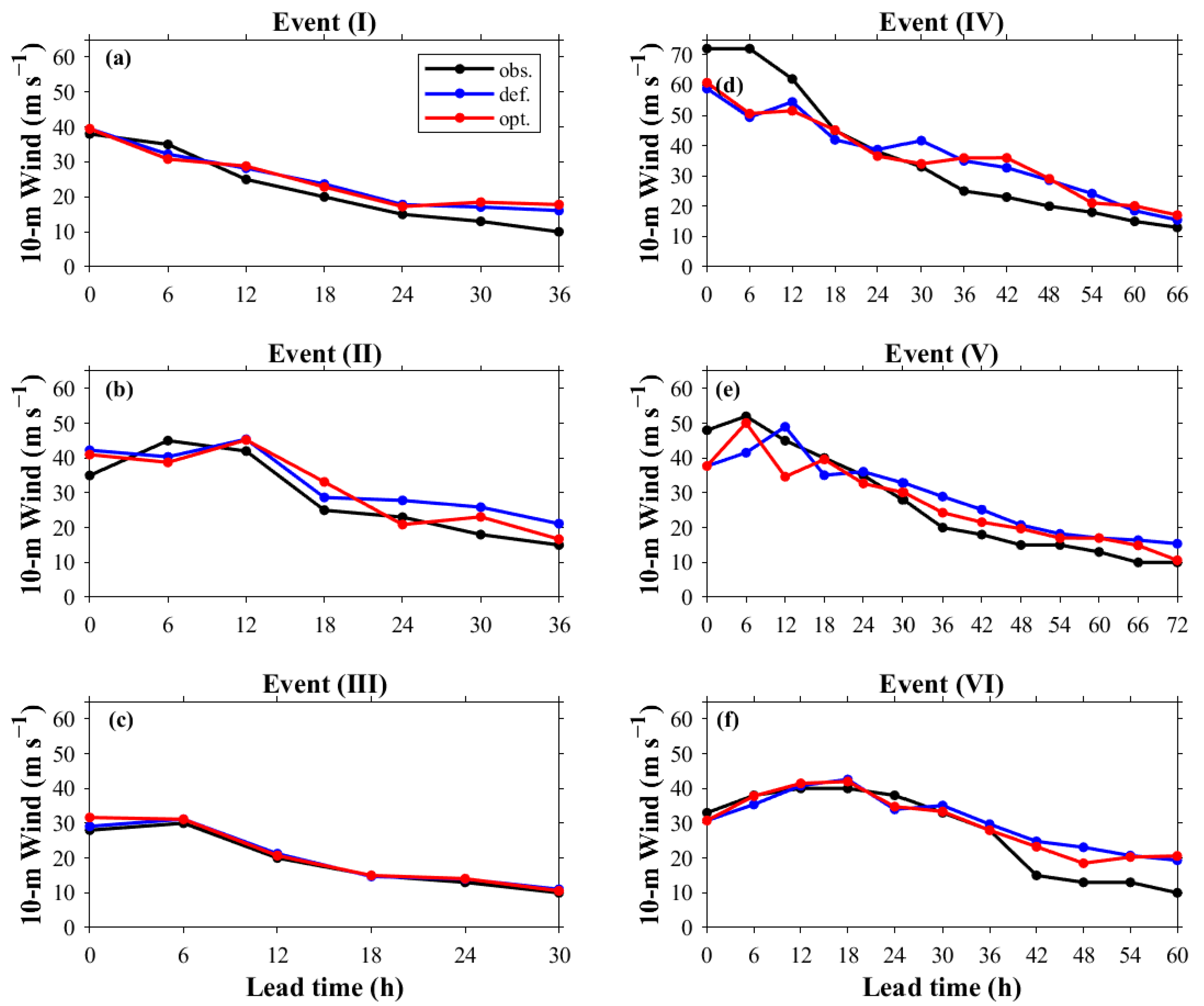
3.4. Validation Analysis of WRF Optimal Parameters
3.5. Parametric Comparison and Physical Interpretation
4. Discussion
5. Conclusions
Supplementary Materials
Author Contributions
Funding
Acknowledgments
Conflicts of Interest
References
- Emanuel, K. Tropical cyclone activity downscaled from NOAA-CIRES reanalysis, 1908–1958. J. Adv. Model Earth Syst. 2010, 2, 1–12. [Google Scholar] [CrossRef]
- Hamill, T.M.; Whitaker, J.S.; Fiorino, M.; Benjamin, S.G. Global ensemble predictions of 2009′s tropical cyclones initialized with an ensemble Kalman filter. Mon. Weather Rev. 2011, 139, 668–688. [Google Scholar] [CrossRef]
- DeMaria, M.; Sampson, C.R.; Knaff, J.A.; Musgrave, K.D. Is tropical cyclone intensity guidance improving? Bull. Amer. Meteor. Soc. 2014, 95, 387–398. [Google Scholar] [CrossRef]
- Chen, X.; Wang, Y.; Zhao, K.; Wu, D. A numerical study on rapid intensification of typhoon Vicente (2012) in the South China Sea. Part I: Verification of simulation, storm-scale evolution, and environmental contribution. Mon. Weather Rev. 2017, 145, 877–898. [Google Scholar] [CrossRef]
- Skamarock, W.C.; Klemp, J.B.; Dudhia, J.; Gill, D.O.; Barker, D.M.; Duda, M.G.; Huang, X.; Wang, W.; Powers, J.G. A description of the Advanced Research WRF Version 3. NCAR Technical Note, NCAR/TN-475 + STR. 2008. Available online: https://opensky.ucar.edu/islandora/object/technotes%3A500/datastream/PDF/view (accessed on 8 June 2008).
- Dudhia, J. A history of mesoscale model development. Asia-Pac. J. Atmos. Sci. 2014, 50, 121–131. [Google Scholar] [CrossRef]
- Kurihara, Y.; Bender, M.A.; Ross, R.J. An initialization scheme for hurricane models by vortex specification. Mon. Weather Rev. 1993, 121, 2030–2045. [Google Scholar] [CrossRef]
- George, J.S.; Jeffries, R.A. Assimilation of synthetic tropical cyclone observations into the Navy Operational Global Atmospheric Prediction System. Weather Forecast. 1994, 9, 557–576. [Google Scholar]
- Zou, X.; Xiao, Q. Studies on the initialization and simulation of a mature hurricane using a variational bogus data assimilation scheme. J. Atmos. Sci. 2000, 57, 836–860. [Google Scholar] [CrossRef]
- Van Nguyen, H.; Chen, Y.L. High-resolution initialization and simulations of Typhoon Morakot (2009). Mon. Weather Rev. 2011, 139, 1463–1491. [Google Scholar] [CrossRef]
- Cha, D.H.; Wang, Y. A dynamical initialization scheme for real-time forecasts of tropical cyclones using the WRF Model. Mon. Weather Rev. 2013, 141, 964–986. [Google Scholar] [CrossRef]
- Li, X. Sensitivity of WRF simulated typhoon track and intensity over the Northwest Pacific Ocean to cumulus schemes. Sci. China Earth Sci. 2013, 56, 270–281. [Google Scholar] [CrossRef]
- Chen, S.; Qian, Y.K.; Peng, S. Effects of various combinations of boundary layer schemes and microphysics schemes on the track forecasts of tropical cyclones over the South China Sea. Nat. Hazards 2015, 78, 61–74. [Google Scholar] [CrossRef]
- Islam, T.; Srivastava, P.K.; Rico-Ramirez, M.A.; Dai, Q.; Gupta, M.; Singh, S.K. Tracking a tropical cyclone through WRF–ARW simulation and sensitivity of model physics. Nat. Hazards 2015, 76, 1473–1495. [Google Scholar] [CrossRef]
- Raju, P.V.S.; Potty, J.; Mohanty, U.C. Sensitivity of physical parameterizations on prediction of tropical cyclone Nargis over the Bay of Bengal using WRF model. Meteorol. Atmos. Phys. 2011, 113, 125–137. [Google Scholar] [CrossRef]
- Chandrasekar, R.; Balaji, C. Sensitivity of tropical cyclone Jal simulations to physics parameterizations. J. Earth Syst. Sci. 2012, 121, 923–946. [Google Scholar] [CrossRef]
- Kanase, R.D.; Salvekar, P.S. Effect of physical parameterization schemes on track and intensity of cyclone LAILA using WRF model. Asia-Pac. J. Atmos. Sci. 2015, 51, 205–227. [Google Scholar] [CrossRef]
- Srinivas, C.V.; Rao, D.V.B.; Yesubabu, V.; Baskaran, R.; Venkatraman, B. Tropical cyclone predictions over the Bay of Bengal using the high-resolution Advanced Research Weather Research and Forecasting (ARW) model. Q. J. R. Meteorol. Soc. 2013, 139, 1810–1825. [Google Scholar] [CrossRef]
- Di, Z.; Gong, W.; Gan, Y.; Shen, C. Combinatorial optimization for WRF physical parameterization schemes: A case study of 3-day typhoon forecasting over the Northwest Pacific Ocean. Atmosphere 2019, 10, 233. [Google Scholar] [CrossRef]
- Jackson, C.S.; Sen, M.K.; Huerta, G.; Deng, Y.; Bowman, K.P. Error Reduction and Convergence in Climate Prediction. J. Clim. 2008, 21, 6698–6709. [Google Scholar] [CrossRef]
- Yang, B.; Qian, Y.; Lin, G.; Leung, R.; Zhang, Y. Some issues in uncertainty quantification and parameter tuning: A case study of convective parameterization scheme in the WRF regional climate model. Atmos. Chem. Phys. 2012, 12, 2409–2427. [Google Scholar] [CrossRef]
- Santanello, J.A.; Kumar, S.V.; Peterslidard, C.D.; Harrison, K.; Zhou, S. Impact of land model calibration on coupled land-atmosphere prediction. J. Hydrometeor. 2013, 14, 1373–1400. [Google Scholar] [CrossRef]
- Duan, Q.; Di, Z.; Quan, J.; Wang, C.; Gong, W.; Gan, Y.; Ye, A.; Miao, C.; Miao, S.; Liang, X.; et al. Automatic model calibration: A new way to improve numerical weather forecasting. Bull. Am. Meteorol. Soc. 2017, 98, 959–970. [Google Scholar] [CrossRef]
- Di, Z.; Duan, Q.; Wang, C.; Ye, A.; Miao, C.; Gong, W. Assessing the applicability of WRF optimal parameters under the different precipitation simulations in the Greater Beijing Area. Clim. Dyn. 2018, 50, 1927–1948. [Google Scholar] [CrossRef]
- Shen, Y.; Zhao, P.; Pan, Y.; Yu, J. A high spatiotemporal gauge-satellite merged precipitation analysis over China. J. Geophys. Res. 2014, 119, 3063–3075. [Google Scholar] [CrossRef]
- Berrisford, P.; Dee, D.; Poli, P.; Brugge, R.; Fielding, M.; Fuentes, M.; Kallberg, P.; Kobayashi, S.; Uppala, S.; Simmons, A. The ERA-Interim Archive Version 2.0; ECMWF: Reading, UK, 2011. [Google Scholar]
- Liu, H.Y.; Wang, Y.; Xu, J.; Duan, Y. A dynamical initialization scheme for tropical cyclones under the influence of terrain. Weather Forecast. 2018, 33, 641–659. [Google Scholar] [CrossRef]
- Wu, J.F.; Xue, X.H.; Hoffmann, L.; Dou, X.K.; Li, H.M.; Chen, T.D. A case study of typhoon-induced gravity waves and the orographic impacts related to Typhoon Mindulle (2004) over Taiwan. J. Geophys. Res. 2015, 120, 9193–9207. [Google Scholar] [CrossRef]
- Dudhia, J.; Gill, D.; Manning, K.; Wang, W.; Bruyere, C. PSU/NCAR Mesoscale Modeling System Tutorial Class Notes and User’s Guide: MM5 Modeling System Version 3; NCAR: Boulder, CO, USA, 1999. [Google Scholar]
- Kain, J.S. The Kain-Fritsch convective parameterization: An update. J. Appl. Meteor. Clim. 2004, 43, 170–181. [Google Scholar] [CrossRef]
- Hong, S.Y.; Lim, J.O.J. The WRF single-moment 6-class microphysics scheme (WSM6). Asia-Pac. J. Korean Meteorol. Soc. 2006, 42, 129–151. [Google Scholar]
- Dudhia, J. Numerical study of convection observed during the winter monsoon experiment using a mesoscale two-dimensional model. J. Atmos. Sci. 1989, 46, 3077–3107. [Google Scholar] [CrossRef]
- Mlawer, E.J.; Taubman, S.J.; Brown, P.D.; Iacono, M.J.; Clough, S.A. Radiative transfer for inhomogeneous atmospheres: RRTM, a validated correlated-k model for the longwave. J. Geophys. Res. 1997, 102, 16663–16682. [Google Scholar] [CrossRef]
- Chen, F.; Dudhia, J. Coupling an advanced land surface–hydrology model with the Penn State–NCAR MM5 modeling system part I: Model implementation and sensitivity. Mon. Weather Rev. 2001, 129, 569–585. [Google Scholar] [CrossRef]
- Hong, S.Y.; Noh, Y.; Dudhia, J. A new vertical diffusion package with an explicit treatment of entrainment processes. Mon. Weather Rev. 2006, 134, 2318–2341. [Google Scholar] [CrossRef]
- Di, Z.; Duan, Q.; Gong, W.; Wang, C.; Gan, Y.; Quan, J.; Li, J.; Miao, C.; Ye, A.; Tong, C. Assessing WRF model parameter sensitivity: A case study with 5 day summer precipitation forecasting in the Greater Beijing Area. Geophys. Res. Lett. 2015, 42, 579–587. [Google Scholar] [CrossRef]
- Di, Z.; Ao, J.; Duan, Q.; Wang, J.; Gong, W.; Shen, C.; Gan, Y.; Liu, Z. Improving WRF model turbine-height wind-speed forecasting using a surrogate- based automatic optimization method. Atmos. Res. 2019, 226, 1–16. [Google Scholar] [CrossRef]
- Shahsavani, D.; Tarantola, S.; Ratto, M. Evaluation of MARS modeling technique for sensitivity analysis of model output. Proc. Soc. Behav. Sci. 2010, 2, 7737–7738. [Google Scholar] [CrossRef]
- Wang, C.; Duan, Q.; Gong, W.; Ye, A.; Di, Z.; Miao, C. An evaluation of adaptive surrogate modeling based optimization with two benchmark problems. Environ. Modell. Softw. 2014, 60, 167–179. [Google Scholar] [CrossRef]
- Duan, Q.; Sorooshian, S.; Gupta, V.K. Optimal use of the SCE-UA global optimization method for calibrating watershed models. J. Hydrol. 1994, 158, 265–284. [Google Scholar] [CrossRef]
- Deb, K.; Pratap, A.; Agarwal, S.; Meyarivan, T. A fast and elitist multiobjective genetic algorithm: NSGA-II. IEEE Trans. Evolut. Comput. 2002, 6, 182–197. [Google Scholar] [CrossRef]
- Gong, W.; Duan, Q.; Li, J.; Wang, C.; Di, Z.; Ye, A.; Miao, C.; Dai, Y. Multiobjective adaptive surrogate modeling-based optimization for parameter estimation of large, complex geophysical models. Water Resour. Res. 2016, 52, 1984–2008. [Google Scholar] [CrossRef]


| No. | Typhoon Events | Simulation Period | Typhoon Period |
|---|---|---|---|
| (1) | 201306 Rumbia | 2013-07-01-08:00–2013-07-04-08:00 | 2013-07-01-08:00–2013-07-02-20:00 |
| (2) | 201409 Rammasun | 2014-07-17-14:00–2014-07-20-14:00 | 2014-07-17-14:00–2014-07-19-20:00 |
| (3) | 201522 Mujigae | 2015-10-03-08:00–2015-10-06-08:00 | 2015-10-03-08:00–2015-10-05-08:00 |
| (4) | 201307 Soulik | 2013-07-12-20:00–2013-07-15-20:00 | 2013-07-12-20:00–2013-07-14-02:00 |
| (5) | 201410 Matmo | 2014-07-22-08:00–2014-07-25-08:00 | 2014-07-22-08:00–2014-07-24-14:00 |
| (6) | 201513 Soudelor | 2015-08-08-02:00–2015-08-11-02:00 | 2015-08-08-02:00–2015-08-10-08:00 |
| Index | Scheme | Parameter | Default | Range | Description |
|---|---|---|---|---|---|
| P3 | Surface layer (module_sf_sfclayrev.F) | znt_zf | 1 | 0.5–2 | Scaling related to surface roughness |
| P4 | karman | 0.4 | 0.35–0.42 | Von Kármán constant | |
| P5 | Cumulus convection (module_cu_kfeta.F) | pd | 1 | 0.5–2 | Scaling related to downdraft mass flux rate |
| P6 | pe | 1 | 0.5–2 | Scaling related to entrainment mass flux rate | |
| P7 | Planetary boundary layer (module_bl_ysu.F) | ph | 150 | 50–350 | Starting height of downdraft above updraft source layer (hPa) |
| P23 | pfac | 2 | 1–3 | Profile shape exponent of the momentum diffusivity |
| No. | Typhoon Events | Simulation Period | Typhoon Period |
|---|---|---|---|
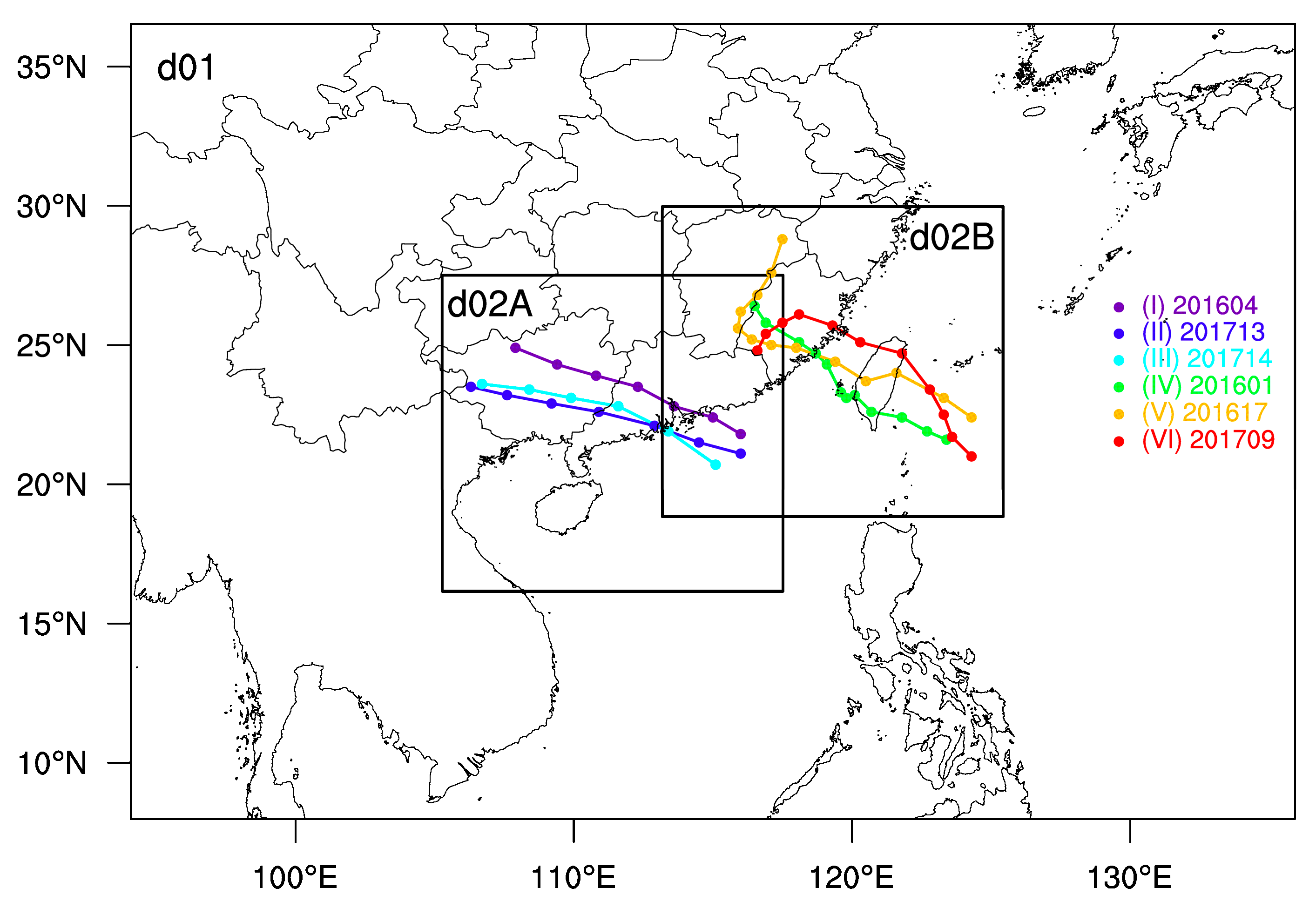
| (I) | 201604 Nida | 2016-08-01-12:00–2016-08-04-12:00 | 2016-08-01-12:00–2016-08-03-00:00 |
| (II) | 201713 Hato | 2017-08-22-18:00–2017-08-25-18:00 | 2017-08-22-18:00–2017-08-25-00:00 |
| (III) | 201714 Pakhar | 2017-08-26-18:00–2017-08-29-18:00 | 2017-08-26-18:00–2017-08-28-00:00 |
| (IV) | 201601Nepartak | 2016-07-07-06:00–2016-07-10-06:00 | 2016-07-07-06:00–2016-07-10-00:00 |
| (V) | 201617 Megi | 2016-09-26-18:00–2016-09-29-18:00 | 2016-09-26-18:00–2016-09-29-18:00 |
| (VI) | 201709 Nesat | 2017-07-28-12:00–2017-07-31-12:00 | 2017-07-28-12:00–2017-07-31-00:00 |
| Name | Precipitation Improved | 10-m Wind Improved |
|---|---|---|
| Run 1 | 8.5% | 6.5% |
| Run 2 | 6.1% | 14.5% |
| Run 3 | 6.8% | 13.6% |
© 2020 by the authors. Licensee MDPI, Basel, Switzerland. This article is an open access article distributed under the terms and conditions of the Creative Commons Attribution (CC BY) license (http://creativecommons.org/licenses/by/4.0/).
Share and Cite
Di, Z.; Duan, Q.; Shen, C.; Xie, Z. Improving WRF Typhoon Precipitation and Intensity Simulation Using a Surrogate-Based Automatic Parameter Optimization Method. Atmosphere 2020, 11, 89. https://doi.org/10.3390/atmos11010089
Di Z, Duan Q, Shen C, Xie Z. Improving WRF Typhoon Precipitation and Intensity Simulation Using a Surrogate-Based Automatic Parameter Optimization Method. Atmosphere. 2020; 11(1):89. https://doi.org/10.3390/atmos11010089
Chicago/Turabian StyleDi, Zhenhua, Qingyun Duan, Chenwei Shen, and Zhenghui Xie. 2020. "Improving WRF Typhoon Precipitation and Intensity Simulation Using a Surrogate-Based Automatic Parameter Optimization Method" Atmosphere 11, no. 1: 89. https://doi.org/10.3390/atmos11010089
APA StyleDi, Z., Duan, Q., Shen, C., & Xie, Z. (2020). Improving WRF Typhoon Precipitation and Intensity Simulation Using a Surrogate-Based Automatic Parameter Optimization Method. Atmosphere, 11(1), 89. https://doi.org/10.3390/atmos11010089