Article

Bulk Scaling Model of Entrainment Zone Thickness in a Convective Boundary Layer, with a Shear Effect Promoted by Velocity Difference

School of Energy and Environment Sciences, Yunnan Normal University, Juxian Road No.798, Kunming 650092, China
*
Author to whom correspondence should be addressed.
Atmosphere 2020, 11(1), 63; https://doi.org/10.3390/atmos11010063
Submission received: 25 October 2019 / Revised: 29 December 2019 / Accepted: 30 December 2019 / Published: 3 January 2020
(This article belongs to the Special Issue Turbulence in Atmospheric Boundary Layers)

Abstract

:
Studying the thickness of the convective boundary layer (CBL) is helpful for understanding atmospheric structure and the diffusion of air pollutants. When there is velocity shear in CBL, the flow field structure is very different from that of shear-free CBL, which makes the thickness model of the entrainment zone deviate. A large-eddy simulation (LES) approach is carried out for a horizontally homogeneous, atmospheric CBL, with a shear effect promoted by velocity difference to explore the bulk scaling model of the entrainment zone thickness. The post-processed data indicate that the existing bulk scaling models cannot synthetically represent the effects of shear and buoyancy on entrainment, resulting in reduced accuracy or limited applicability. Based on the fraction of turbulent kinetic energy (TKE) used for entrainment, a different form of the characteristic velocity scale, which includes the shear effect, is proposed, and a modified bulk scaling model that uses a potential temperature gradient to replace the potential temperature jump across the entrainment zone is constructed with the numerical results. The new model is found to provide an improved prediction of the entrainment zone thickness in a sheared CBL.

1. Introduction

Due to the compound influence of surface radiation, potential temperature gradient (also named inversion strength), wind shear, and other factors, the flow field in a sheared convective boundary layer (CBL) is complex; this is especially true in the entrainment zone formed by shear and buoyancy between the mixed zone and the free atmosphere, which restricts the exchange of matter and heat between the layers. Accurately describing and quantifying the thickness of the entrainment zone in a sheared CBL is of significance for meteorological prediction [1,2], as well as numerous environmental and engineering applications [3,4].
The current bulk scaling models for the entrainment zone are primarily based on the CBL framework of a “zero-order model” (ZOM) [5] and a “first-order model” (FOM) [6]. An FOM assumes a linear variation of parameters with height in the CBL, which is more consistent with the observed data. The height of the entrainment zone, z i , as sketched in Figure 1, is defined by the level of the buoyancy flux minimum w θ ¯ | i , and the upper limit of the entrainment zone, z 2 , is the zero-crossing height of the buoyancy flux profile, using linear interpolation between discrete grid points. The height of the mixed zone, z 1 , takes the corresponding level of zero buoyancy flux. Due to the large-scale turbulent eddies in the entrainment zone, it is difficult to accurately locate the height of zero buoyancy flux in the upper layer, and Fedorovich et al. [7] and Conzemius and Fedorovich [3,4] adopted the height at which the buoyancy flux returns 90% of the way back to zero from its grid minimum as z 2 . Similarly, in order to eliminate the influence of the inhomogeneity of thermals in the surface layer, the corresponding position of 5~10% of the surface buoyancy flux is taken as the height of the underlying surface, z S .
In a shear-free CBL, Turner and Benton [8] and Vanzanten et al. [9] concluded that the development of the CBL mainly depends on the turbulence process and the potential temperature change in the entrainment zone. Stull [10] and Zeman and Tennekes [11] established a bulk scaling model for the entrainment zone thickness, based on the conservation of kinetic and potential energy of thermals in the zone, as follows:
Δ z / z i R i * 1 ,
where the convective Richardson number R i * is defined as
R i * = g θ 0 Δ θ z i / w * 2 ,
and the convective velocity scale w * is given by
w * = ( g θ 0 w θ | s ¯ z i ) 1 / 3 ,
in which θ 0 is the ambient virtual potential temperature and g is the gravitational acceleration.
With their convective water tank experiments, Deardorff et al. [12] obtained the following correlation for the above bulk scaling model:
Δ z / z i = 1.31 R i * 1 + 0.21 .
This correlation is denoted as Model 1 in this study. However, there is no consensus on such a bulk scaling model. For example, Boers [13] obtained a (−1/2) power-law correlation, while Beyrich and Gryning [14] concluded that there is no such correlation through their analysis of lidar measured data.
Gryning and Batchvarova [15] adopted the entrainment velocity w e ( w e = d z i / d t ) instead of w * as the velocity scale, and constructed the following bulk scaling model in terms of the entrainment Richardson number R i E :
Δ z / z i = 3.3 R i E 1 / 3 + 0.2 ,
where R i E is defined as
R i E = g θ 0 Δ θ z i / w e 2 .
This model is denoted as Model 2 in this study. Model 2 was found to agree well with the measured atmospheric data of Boers and Eloranta [16].
When there is velocity difference at the entrainment zone, a significant shear effect will enhance the entrainment process. For sheared CBL, Kim et al. [17] suggested that the bulk scaling model for Δ z / z i should include the influence of the shear effect, and a modified convective Richardson number defined below, which takes into account the shear effect, should be used instead:
R i * = g θ 0 Δ θ z i / w m 2 ,
in which a new velocity scale is given by
w m 2 = w * 2 + a u * 2 + b ( Δ U 2 + Δ V 2 ) ,
where a and b are constants, Δ U and Δ V are the jumps of the x- and y-component velocity across the entrainment zone, and the friction velocity scale is
u * = u w ¯ | s .
The modified R i * , using w m in place of w * as the velocity scale, takes full account of the buoyancy and shear effects on entrainment. With such a modified convective Richardson number, Kim et al. [17] gave the following three bulk scaling models:
Δ z / z i = 0.075 R i * 1 + 0.0925 ,   with   w m 2 = w * 2 + 180.21 u * 2 + 0.15 ( Δ U 2 + Δ V 2 ) ;
Δ z / z i = 2.68 R i * 1 ,   with   w m 2 = w * 2 + 2.99 u * 2 + 0.03 ( Δ U 2 + Δ V 2 ) ;
Δ z / z i = 1.12 R i * 1 + 0.08 ,   with   w m 2 = w * 2 + 4 u * 2 + 0.1 ( Δ U 2 + Δ V 2 ) ,
which are denoted in this study as Model 3, Model 4, and Model 5, respectively.
Heng et al. [18] validated above models with their large-eddy simulation (LES) numerical results, and showed that the entrainment zone thickness predicted by Model 4 is consistent with the data of the barotropic and baroclinic atmosphere; however, the values of the proportional coefficients lead to deviations between the predicted results by the models and the numerical results.
As the potential temperature gradient in the free atmosphere layer plays a key role in the entrainment process, Hageli et al. [19], Fedorovich et al. [7], and Jianning et al. [20] proposed the following three models (denoted here as Model 6, Model 7, and Model 8, respectively) in terms of the buoyancy Richardson number RiN:
Δ z / z i = C 1 R i N 1 / 2 ,
Δ z / z i = C 2 R i N 2 / 5 ,
Δ z / z i = C 3 R i N 1 / 3 ,
where C1, C2, and C3 are constants, and R i N is defined as
R i N = z i 2 N 2 w * 2 ,
in which N is the Brunt-Väisälä frequency, and N 2 = ( g / θ 0 ) Γ θ .
Extensive field observations and lab water tank experiments have shown that the fluctuations of the buoyancy flux near zero in the upper entrainment zone cause large deviations in the determination of the upper limit of z 2 [7,12,19,21], which makes the determination of Δ θ very difficult, and weakens the linearity of the fitted results of Δ z / z i . Hence, Jianning et al. [20] took Γ θ instead of Δ θ as the atmospheric stability parameter, in order to improve the accuracy of the fitted relationship, and obtained another form of the bulk scaling model (denoted here as Model 9) based on the energy relationship of thermals in the entrainment zone:
Δ z z i = C 4 ( θ * Γ θ z i ) 1 / 2 ,
where C4 is a constant, and the potential temperature scale θ * is defined as
θ * = w θ ¯ | s / w * .
The authors obtained C 4 = 1.44 with the data of Deardorff et al. [12] and Boers and Eloranta [16], but it was found that Model 9 failed to reflect the effect of the shear on the entrainment process.
In summary, shear stress in the CBL makes the bulk scaling models for the entrainment zone thickness based on shear-free CBL deviate significantly, because the models fail to take into account the compounding influence of characteristic parameters of the sheared CBL. In this paper, numerical cases using LES are carried out in an atmospheric domain, with different combinations of Δ U , Γ θ , and w θ ¯ | i , and the nine models identified above are examined. Finally, a modified bulk scaling model for the entrainment zone thickness for sheared CBL is developed with the LES results obtained.

2. Numerical Methodology

2.1. LES Description

LES decomposes the instantaneous motion of a turbulent eddy in the flow regime by some filtering function into two parts: a large-scale eddy and a small-scale eddy. LES computes the large-scale components directly and models the subgrid scales via a subgrid-scale (SGS) model that represents the effect of the unresolved scales on the resolved ones. As LES can capture the large-scale effects and coherent structures in unsteady processes, adequately reflecting the turbulent characteristics and overcoming the huge computational cost of direct numerical simulation, it has been widely used in the research of the atmospheric boundary layer [7,22,23].
For a horizontally homogeneous turbulent flow, the filtered governing equations are as follows:
u i ¯ x i = 0 ,
u i ¯ t + x j ( u i ¯ u j ¯ ) = ν t [ ( u i ¯ x j + u j ¯ x i ) 2 3 u l ¯ x l δ i j ] 1 ρ p ¯ x i τ i j x j ,
θ ¯ t + u i ¯ θ ¯ x i = x i ( λ ρ C p θ ¯ x i ) + 1 ρ C p ( p ¯ t + u j ¯ p ¯ x i ) τ θ i x j ,
where ui and uj are the velocity vectors with components along the directions xi and xj; ρ is the density; ν is the kinematic viscosity; τ i j is the subgrid-scale (SGS) stress; δij is Kronecker delta; Cp and λ are the specific heat capacity at constant pressure and thermal conductivity, respectively; and τ θ i is the SGS turbulence flux of the virtual potential temperature. This is modeled by using an SGS turbulent Prandtl number:
τ θ i = ν S G S Pr S G S θ ¯ x j ,
in which ν S G S is SGS viscosity and Pr S G S is the SGS Prandtl number. The SGS turbulent stresses are calculated by
τ i j = 1 3 τ k k δ i j 2 ν S G S S i j ¯ .
As for incompressible flows in the CBL, the isotropic part of the SGS stress τ k k can be neglected, as the turbulent velocity scale is too small. The rate-of-strain tensor for the resolved scale S ¯ i j is defined by
S i j ¯ = 1 2 ( u i ¯ x j + u j ¯ x i ) .
In this study, the SGS model adopts eddy viscosity (νSGS) as the following [24]:
ν S G S = [ min ( k d , C S G S Δ ) ] 2 2 S i j ¯ S i j ¯ ,
where k is the von Kármán constant; d is the distance to the closest wall; C S G S is the model coefficient, which is estimated based on the dynamic procedure; and Δ represents the local grid scale based on the cell volume Δ = V 1 / 3 .
Recent studies [25,26,27] have addressed that LES has some difficulties in getting entrainment layer dynamics right. These difficulties are mainly attributed to overestimation of eddy viscosity due to an excessive velocity gradient in the entrainment process. That is to say, C S G S cannot cover all cases with a universal constant. In an attempt to address these deficiencies, we therefore perform the dynamic Smagorinsky–Lilly SGS Model [28], in which C S G S is dynamically computed based on the information provided by the resolved scales of motion, which changes with the time of calculation and the spatial position of discrete points in the domain. In addition, other efforts have been made, such as reducing the grid spacing and solving the governing equations by using the central difference to eliminate the oscillation of the solution.

2.2. Large-Eddy Simulation Setup

Fitzjarrald [29] and Hadfield et al. [30] estimated the aspect ratio of the tank to be at least 4.5 to eliminate the sidewall influence on the central eddies in convective water tank experiments. Although the empirical value is based on the water tank, it is still valuable for the determination of computational domain size, and even an indication that even larger values are desirable was provided by some recent large-eddy simulations [31]. This paper carries out the LES runs in a horizontally homogeneous atmospheric domain of 6000 × 6000 × 2000 m3 (X × Y × Z) with an aspect ratio of 6 (the initial entrainment zone height is 1000 m).
The bulk of the computational domain is meshed by the grid size of 50 m × 50 m × 25 m, which is similar to that of Sullivan et al. [32], Fedorovich et al. [7], and Gentine et al. [33]. Because the vertical turbulent kinetic energy (TKE) distribution is not uniform, with buoyancy- and shear-generated TKE mainly concentrated in the underlying surface sublayer and the entrainment zone, the grid size near the surface varies steadily from 3 to 25 m and 15 m of the entrainment zone. Some tests are conducted to examine the numerical solutions’ sensitivity to grid resolution, and the result shows that the means and second-order statistics from the simulations on the chosen grid and a bigger grid (100 m × 100 m × 20 m) differ by no more than 5%, indicating that the current grid resolution provides accurate solutions.
The upper boundary is specified as a symmetrical rigid lid, where the vertical fluxes of physical parameters, such as mass, momentum, heat, and subgrid kinetic energy fluxes, are zero. As statistical characteristics of steady CBL turbulence are almost horizontally uniform, all runs are performed using periodic boundary conditions at the streamwise and side walls, as well as the no-slip boundary condition with constant buoyancy flux at the underlying surface.

2.3. Initial Conditions and Data Post-Processing

The simulated cases are uniformly initialized with an entrainment zone height of 1000 m, below which the potential temperature profile is at a constant 300 K, and above which it increases with a gradient Γ θ . The horizontal velocities of the mixed zone and the free atmosphere are U 1 and U 2 , respectively, and the velocity difference at the interface between the upper and lower zones is Δ U ( Δ U = U 2 U 1 ), in order to generate wind shear.
In this study, we consider different sheared CBLs by prescribing a series of combinations of Δ U , Γ θ , and w θ ¯ | s , as listed in Table 1, of which the main characteristic data are consistent with the actual atmospheric range, as presented in Table 2; thus, the simulation results are comparable with the actual atmospheric data.
The momentum equation is discretized by the finite volume method, and the pressure–velocity coupling algorithm is based on the PISO (pressure implicit with splitting of operators) scheme [34]. The unsteady calculation time step of all simulations was 0.2 s, and the quasi-steady calculation time satisfies the experiential requirement of t > 6 t * [35], where the time scale t * is t * = z i / w * , ensuring the TKE does not change significantly with time, and the flows are in a stable development stage at the end of the simulation.
Three-dimensional data volumes were archived from the final stage of the simulations to gather statistics and present flow visualization. The ensemble mean and turbulence statistics shown here are the result of spatial averaging—that is, at a fixed z location averaged over a x–y plane.

3. Evaluation of the Existing Bulk Models

3.1. Thickness of the Entrainment Zone

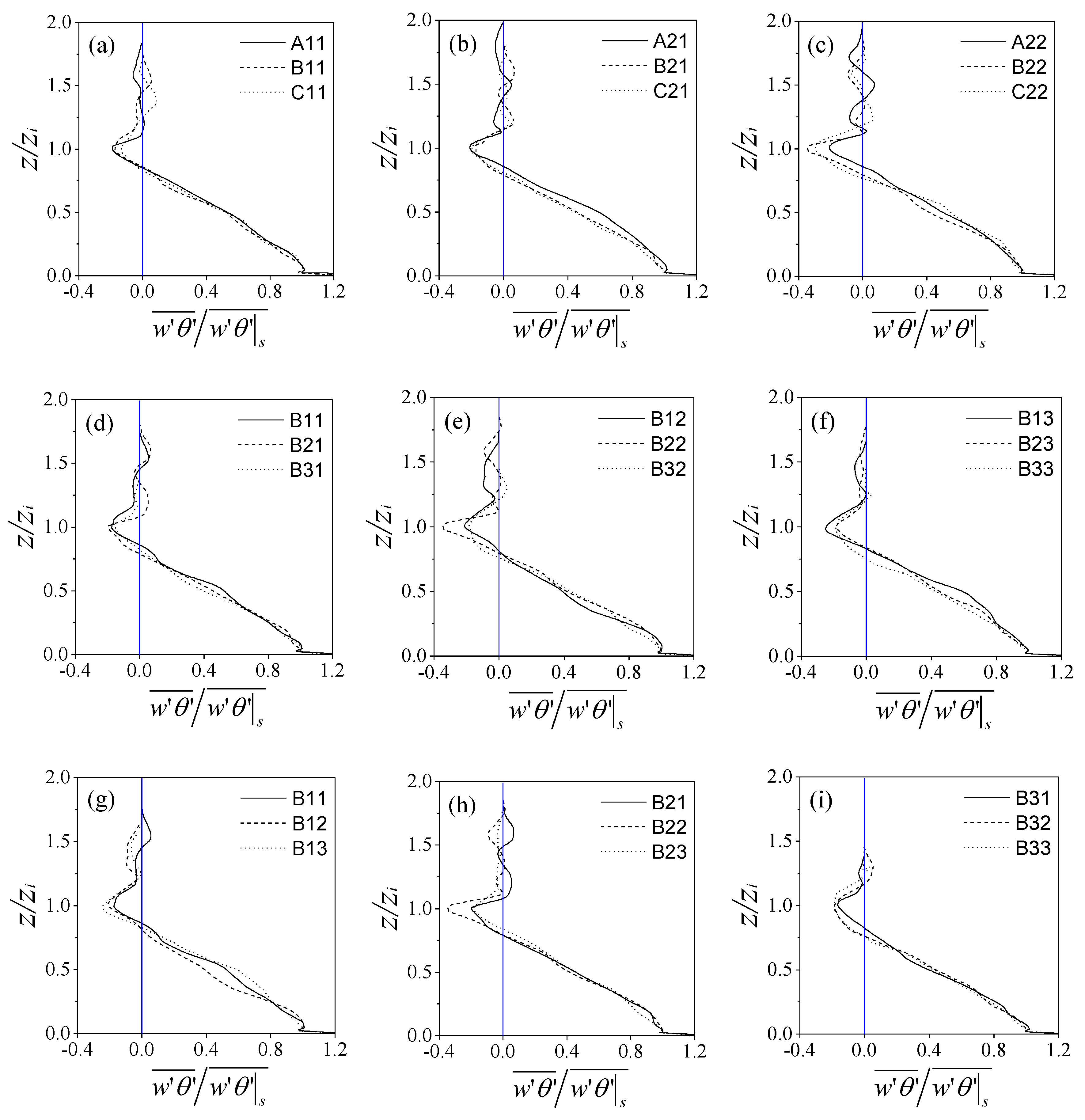
Since horizontal averages may be taken as substitutes for the ensemble averages in the horizontally homogeneous CBL, the horizontally averaged flow statistics are assumed to converge to corresponding ensemble means. From this point forward, the buoyancy flux of all grid nodes in the computational domain is averaged horizontally, in order to obtain the vertical buoyancy flux profiles of all simulated cases, as illustrated in Figure 2.
Figure 2 presents the evolution of the vertical profiles of buoyancy flux, which is made dimensionless by the surface buoyancy flux w θ ¯ | s , obtained from the LES results. The surface buoyancy flux is a major turbulence production mechanism in atmospheric boundary layer, and a stronger surface buoyancy flux enlarges the temperature difference between the thermals from the surface sublayer and the ambience, which determines the depth of the thermals penetrating into the free atmosphere and decisively impacts the entrainment development. From Figure 2a–c, it is seen that the increase of w θ ¯ | s from 0.05 K·m/s to 0.15 K·m/s expands Δ z by 10 to 70 m, indicating that the promotion of entrainment and its influence is particularly strong in cases with a weak stratified environment (the cases with smaller Γ θ , i.e., A11, B11, C11), which is consistent with the analysis for shear-free CBLs [37].
As the behavior of thermals in the CBL is dominantly affected by negative buoyancy, the inhibition of entrainment by the potential temperature gradient of the free atmosphere is very obvious by comparing Figure 2d–f, and Δ z significantly shrinks with the strengthening of Γ θ . From the figure, it can be seen that the inhibition effect of Γ θ is relatively obvious to z 2 , especially in the cases of weak surface buoyancy flux (Figure 2d), as Γ θ increases the resistance of the thermals to uprush. This is consistent with the simulated results of Boers and Eloranta [16] and the lidar observations of Hageli et al. [19].
Kim et al. [17] and Pino et al. [38] elucidated that the vertical shear stress of the horizontal wind destroyed the stability of the Kelvin–Helmholtz wave at the interface and enhanced entrainment. The thickness of the entrainment zone is directly related to the strength of the velocity difference under the same w θ ¯ | s and Γ θ conditions, as shown in Figure 2g–i, especially in the case of weak inversion strength (smaller Γ θ ), where Δ z increases more remarkably. For example, when Δ U is increased from 1.5 m/s to 3 m/s, the Δ z of the B31 case increased 65 m over that of the B32 case, while the B22 case increased only 28 m over the B21 case. This reveals that the turbulence intensity in the entrainment zone with weak inversion strength is smaller, and the shear-generated TKE consumed by the negative buoyancy in the entrainment zone increases accordingly, which makes the thickness increase more.
From the above observations, it is found that the characteristic factors of the boundary layer, i.e., Δ U , Γ θ , and w θ ¯ | s have significant influence on the development of the entrainment zone, with both Δ U and w θ ¯ | s promoting entrainment and Γ θ inhibiting the entrainment process. Therefore, these parameters must be taken into account collectively, in order to obtain the bulk scaling models that are able to provide accurate predictions.

3.2. Evaluation of the Existing Bulk Models

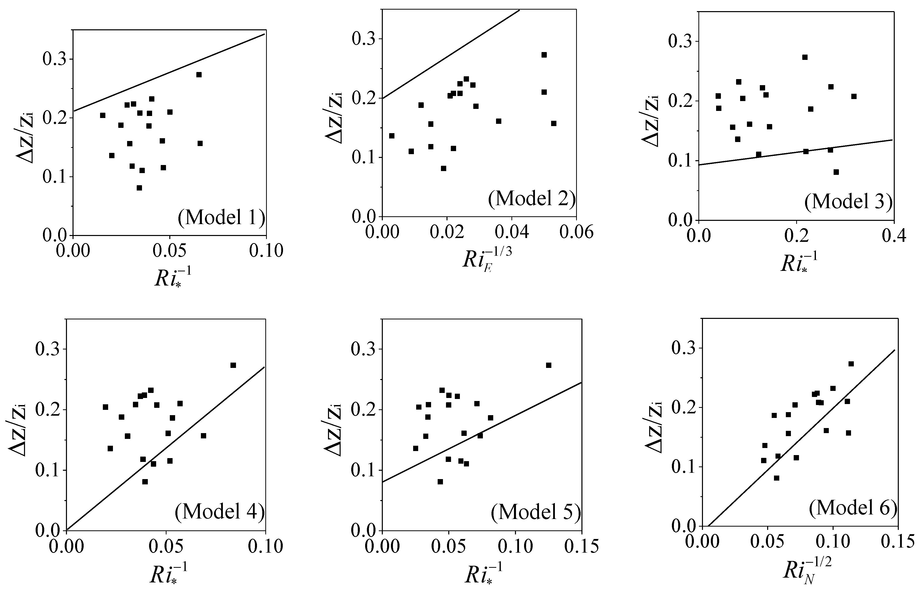
The numerical results of the LES cases obtained in this study can be used to evaluate the accuracy of the bulk scaling models presented above, i.e., Models 1–9. The results of the evaluation are presented in Figure 3. The results show that the use of the shear-free velocity scale w * in R i * of Model 1, which does not includes the effect of shear in the entrainment zone, making the predictions by the model deviate substantially from the numerical results. Model 2 uses the entrainment velocity w e as the velocity scale, which implicitly reflects the influence of the CBL characteristic factors on entrainment. However, the predicted results are not in agreement with the numerical results.
Models 3–5 use the fraction velocity scale of the underlying surface and the velocity difference of the entrainment zone in the velocity scale, involving the shear effects occurring in both discrete sublayers of the sheared CBL. Deardoff and Willis [39] and Moeng and Sulliwan [40] concluded that shear-generated TKE is quickly dissipated by molecular viscous at a short depth before it can be utilized to drive the entrainment process through the entire mixed zone. Conzemius and Fedorovich [3,4] argued that the surface friction affects the vertical evolution of momentum and it has almost no impact on the entrainment process, through the simulation of typical daytime atmospheric CBLs. The overestimation of the contribution of the surface friction velocity in the velocity scale of Model 3 results scatters the numerical data more, and the correlations between Δ z / z i and R i * 1 cannot be clearly seen from the figure. The predictions from Models 4 and 5 agree reasonably well with the numerical results, although they systematically underestimate the results.
There is a large statistical deviation in the determination of the upper limit of the entrainment zone, which reduces the reliability of the derived models. However, this is supposed to be improved by replacing Δ θ with Γ θ in the bulk scaling model. Models 6–8 proposed the scaling relationship between the dimensionless thickness and the buoyancy Richardson number R i N with such a replacement. From the figure, it is clear that Δ z / z i and R i N are in good agreement with the −1/2 to −1/3 power-law correlations, which is in agreement with the conclusions from relevant studies, as mentioned above. However, because w * is still used as the velocity scale in these models, it excludes the effect of the shear; whether the accuracy of the models can be improved requires further study.
The temperature scale θ * , which implicitly reflects the influence of the surface buoyancy flux, is taken as the entrainment index in Model 9. The LES results presented in Figure 3 show that Model 9 improves the predictions. It is noteworthy that Model 9 cannot describe a clear entrainment process in sheared CBL, due to the lack of consideration of the shear effect on entrainment.
In conclusion, compared with the shear-free R i * 1 model (Model 1), the velocity scales w e and w m in Models 2–5 include the influence of the shear effect on entrainment, which are comparatively more in line with the numerical results (except for Model 3, due to the extensive estimation of the surface shear effect). In Models 6–8, R i N uses Γ θ instead of Δ θ as the inversion strength parameter in the prediction of the models. Although the prediction is much improved, Model 9 does not take into account of the effect of Δ U on the entrainment process, resulting in some limitations of its application.

4. Improved Bulk Scaling Models in a Sheared Convective Boundary Layer

4.1. Development of the Improved Bulk Scaling Model

The shear-generated TKE in the entrainment zone is partly dissipated by the molecular viscosity in the turbulent flow, and the remainder is balanced by the negative buoyancy. The vertical motion of thermals in the mixed zone can effectively relax the turbulence of the mean wind in the middle of CBL, so that the shear-generated TKE at the surface can be dissipated within a short distance, thus reducing the upward transport of TKE. The shear at the surface has little effect on entrainment compared with the shear in the entrainment zone, as illustrated in water tank experiments and numerical simulations [7,16,39]. Therefore, the varied coefficient of u * in Equation (8) (i.e., a) is not sensitive enough to change the value of the velocity scale remarkably; therefore, it is feasible to ignore u * in the velocity scale without a significant impact on the model.
Based on the ZOM framework, Conzemius and Fedorovich [3,4] defined Cp as the ratio of the integral of the buoyancy flux difference with shear-free cases to the integral shear production between z s and z 2 , and found that Cp was in the range of 0.2~0.5, with an average value of 0.35 in the sheared CBL atmospheric cases:
C p = g θ 0 0 z 2 w θ ¯ d z 0.4 w θ | s ¯ z s z 2 ( τ x u z + τ y v z ) d z ,
where the shear stress components are τ x = w u ¯ and τ y = w v ¯ . We then suggest the following modified w m :
w m 2 = w * 2 + C p ( Δ U 2 + Δ V 2 ) ,
where Cp is the fraction of the shear-generated TKE available for entrainment. At the end of the calculation, the horizontal velocity components of the mixed layer are basically constant, due to the vertical turbulent mixing of the rising motion of the thermals, and the horizontal velocity of the free atmosphere is basically unaffected by the entrainment of the lower layer.
According to the thermal parcel theory, the negative buoyancy ( ρ ρ 0 ) g in the entrainment zone ( z i ~ z 2 ) decelerates the upward movement of the thermals, from w m at the top of the mixed zone to zero when it reaches the top of the entrainment zone. The vertical energy conservation equation of thermals’ overshooting in the zone to resist negative buoyancy can be written as
0 1 2 ρ 0 w m 2 = z i z 2 ( ρ ρ 0 ) g d z ,
where ρ 0 is ambient atmospheric density. The left-hand side of the equation is the change of the kinetic energy of thermals, and the right-hand is the integrated buoyancy-generated work budget in the entrainment zone.
As the CBL is finite in height relative to the earth’s atmosphere, the effect of pressure on its density is negligible, but gravity is sufficiently strong. Therefore, the local density mainly depends on the potential temperature profile, and could be written as following with the Boussinesq approximation:
ρ = ρ 0 [ 1 1 θ 0 ( θ θ 0 ) ] .
The entrainment zone thickness is mainly extruded by the potential temperature gradient of the free atmosphere in the CBL. Sun et al. [20] found an approximation between the potential temperature jump and its gradient in the entrainment zone, using the experimental data of Deardorff et al. [12] and the numerical data of Fedorovich et al. [7]:
Δ θ / Δ z = β Γ θ .
With Equations (29) and (30), the right-hand side of Equation (28) can be written as
z i z 2 ( ρ ρ 0 ) g d z = ρ 0 g β Γ θ ( Δ z ) 2 2 θ 0 ;
Thus, Equation (28) can be expressed as
1 2 ρ 0 w m 2 = ρ 0 g β Γ θ ( Δ z ) 2 2 θ 0 .
That is,
Δ z z i = ( g / θ 0 β Γ θ z i 2 w m 2 ) 1 / 2 = β 1 / 2 R i N C 1 / 2 ,
where R i N C is the corrected Richardson number by the shear effect, defined as R i N C = N 2 z i 2 / w m 2 , and w m is in the modified form expressed by Equation (26).

4.2. Comparison of the Improved Model Against the Available Data

Otte and Wyngaard [41] simulated both shear-free and sheared atmospheric CBL in the range of 2~4.2 km, and obtained the vertical distributions of the potential temperature and velocity. The development of remote sensing technology has enabled us to simultaneously measure the parameters of the whole CBL. Boers and Eloranta [16] used lidar and a pilot balloon to measure the dry atmospheric data in the center of Illinois for six uninterrupted days in June 1979, and captured the vertical profiles of temperature and wind velocity in the CBL, as well as the surface heat flux, friction velocity, etc. Lothon et al. [42] used National Oceanic and Atmospheric Administration (NOAA) high-resolution doppler lidar (HRDL) to measure CBL parameters to determine the position of the entrainment zone.
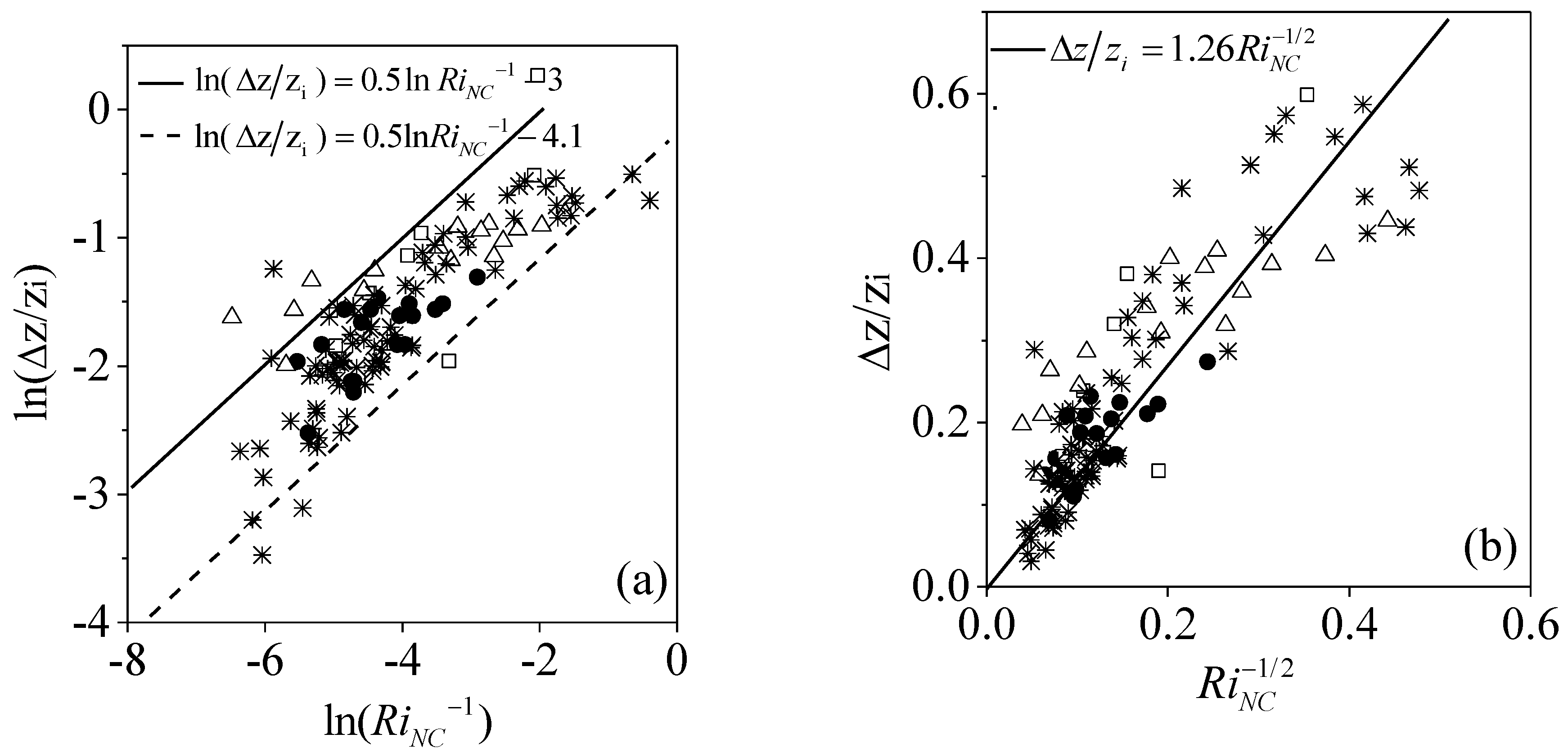
With the aid of the data from these lidar measurements and numerical simulations, we fit the relationship between Δ z / z i and R i N C with the developed, improved model, and present the results in Figure 4. The following quantified scaling model is obtained from the presented data:
Δ z z i = 1.26 R i N C 1 / 2 .
In this paper, Cp takes the statistical average of the turbulence simulation, but it is in fact related to the development process and entrainment factors of CBL. To date, the specific mechanism and rules of CBL are not very clear, and it is necessary to fully understand the entrainment process in future studies.
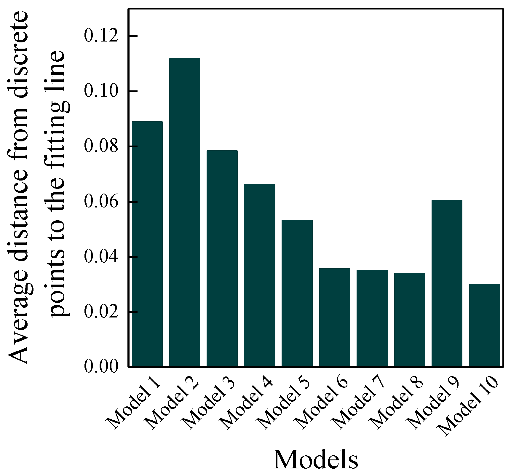
We took the average distance from the discrete points to the fitting lines as the index to describe the quality of models in Figure 3 and the new model (Equation (34), denoted as Model 10) in Figure 4. It can be seen from Figure 5 that the model developed in the current study provides an improved prediction.

5. Conclusions

In this study, LES was carried out to simulate the sheared CBL cases in a horizontally homogeneous atmospheric domain. The behaviors of the nine current bulk scaling models between the dimensionless entrainment zone thicknesses and different Richardson numbers ( R i * , R i E , R i N ) and θ * / ( Γ θ z i ) were evaluated against the LES results. The following conclusion can be drawn:
  • The traditional R i * model does not include the shear effect on entrainment, and thus does not perform well in the sheared CBL. Using w m as the velocity scale to include the shear effect on entrainment, the revised R i * model provides some improvement in the predictions, but still with large deviations due to the large deviations in determining Δ θ in the entrainment zone.
  • For the correlation with Δ θ , Γ θ is adopted as the influence factor of inversion stratification on entrainment process in the R i N model, which reduces the deviations of the predictions. However, this model is mainly aimed at a shear-free CBL, and also fails to take into account of the shear effect.
  • In the R i E model, the entrainment velocity w e at the interface is used as the velocity scale, which implicitly involves the comprehensive influence of buoyancy and shear on the entrainment process. However, each influence factor on the process cannot be quantified clearly, and the predictions are not very accurate.
  • Similarly, due to the exclusion of the shear effect on entrainment, the “ θ * / ( Γ θ z i ) ” model also has some limitations in the predictions for sheared CBL.
A characteristic velocity scale w m based on the fraction of TKE used for entrainment, which includes the shear effect, was constructed in this study, and an improved bulk scaling model with this revised velocity scale has been derived from the modification of the previous methods and theoretical analysis of energy conservation in the entrainment process. The model uses w m and Γ θ as characteristic parameters, which fully reflects the influence of the boundary layer characteristic factors on the entrainment process. The correlation predicted by this model has been shown to provide significantly improved predictions.

Author Contributions

Evolution of overarching research goals and aims, A.L. and T.L.; formulation or evolution of overarching research goals and aims, W.G. and T.L.; conducting research, performing the numerical experiments, and data processing, A.L.; creation and analysis of models, A.L. and W.G.; writing the initial draft, A.L. All authors have read and agreed to the published version of the manuscript.

Funding

This research was funded by the National Natural Science Foundation of China, grant number 11662021.

Acknowledgments

This work received generous help from Computational Fluid Dynamics Laboratory of the Solar Energy Research Institute of Yunnan Normal University. The authors of this paper gratefully thank all those who provided help.

Conflicts of Interest

The authors declare no conflict of interest. The funders had no role in the design of the study; in the collection, analyses, or interpretation of data; in the writing of the manuscript, or in the decision to publish the results.

References

  1. Ackerman, A.S.; Kirkpatrick, M.P.; Stevens, D.E.; Toon, O.B. The impact of humidity above stratiform clouds on indirect aerosol climate forcing. Nature 2004, 432, 1014–1017. [Google Scholar] [CrossRef]
  2. IPCC. Climate Change 2007: The Physical Science Basis. In Contribution of Working Group I to the Fourth Assessment Report of the Intergovernmental Panel on Climate Change; Cambridge University Press: Cambridge, UK; New York, NY, USA, 2007; p. 996. [Google Scholar]
  3. Conzemius, R.J.; Fedorovich, E. Dynamics of sheared convective boundary layer entrainment. Part I: Methodological background and large-eddy simulations. J. Atmos. Sci. 2006, 63, 1151–1178. [Google Scholar] [CrossRef] [Green Version]
  4. Conzemius, R.J.; Fedorovich, E. Dynamics of sheared convective boundary layer entrainment. Part II: Evaluation of bulk model predictions of entrainment flux. J. Atmos. Sci. 2006, 63, 1179–1199. [Google Scholar] [CrossRef] [Green Version]
  5. Lilly, D.K. Models of cloud-topped mixed layers under a strong inversion. Q. J. R. Meteorol. Soc. 1968, 94, 292–309. [Google Scholar] [CrossRef]
  6. Betts, A.K. Non-precipitating cumulus convection and its parameterization. Q. J. R. Meteorol. Soc. 1973, 99, 178–196. [Google Scholar] [CrossRef]
  7. Fedorovich, E.; Conzemius, R.; Mironov, D. Convective entrainment into a shear-Free, linearly stratified atmosphere: Bulk models reevaluated through large eddy simulations. J. Atmos. Sci. 2004, 61, 281–295. [Google Scholar] [CrossRef] [Green Version]
  8. Turner, J.S.; Benton, E.R. Buoyancy Effects in Fluids. Phys. Today 1974, 27, 52–53. [Google Scholar] [CrossRef]
  9. Vanzanten, M.C.; Duynkerke, P.G.; Cuijpers, J.W.M. Entrainment parameterization in convective boundary Layers. J. Atmos. Sci. 1999, 56, 813–828. [Google Scholar] [CrossRef]
  10. Stull, R.B. Inversion rise model based on penetrative convection. J. Atmos. Sci. 1973, 30, 1092–1099. [Google Scholar] [CrossRef] [Green Version]
  11. Zeman, O.; Tennekes, H. Parameterization of the turbulent energy budget at the top of the daytime atmospheric boundary layer. J. Atmos. Sci. 1977, 34, 111–123. [Google Scholar] [CrossRef] [Green Version]
  12. Deardorff, J.W.; Willis, G.E.; Stockton, B.H. Laboratory studies of the entrainment zone of a convectively mixed layer. J. Fluid. Mech. 1980, 100, 41–64. [Google Scholar] [CrossRef]
  13. Boers, R. A parameterization of the depth of the entrainment zone. J. Appl. Meteorol. 1989, 28, 107–111. [Google Scholar] [CrossRef] [Green Version]
  14. Beyrich, F.; Gryning, S.E. Estimation of the entrainment zone depth in a shallow convective boundary layer from sodar data. J. Appl. Meteorol. 1998, 37, 255–268. [Google Scholar] [CrossRef]
  15. Gryning, S.E.; Batchavarova, E. Parameterization of the depth of the entrainment zone above the daytime mixed layer. Q. J. R. Meteorol. Soc. 1994, 120, 47–58. [Google Scholar] [CrossRef]
  16. Boers, R.; Eloranta, E.W. Lidar measurements of the atmospheric entrainment zone and the potential temperature jump across the top of the mixed layer. Bound. Layer Meteorol. 1986, 34, 357–375. [Google Scholar] [CrossRef]
  17. Kim, S.W.; Park, S.U.; Pino, D.; Arellano, J.V.G. Parameterization of entrainment in a sheared convective boundary layer using a first-order jump model. Bound. Layer Meteorol. 2006, 120, 455–475. [Google Scholar] [CrossRef] [Green Version]
  18. Heng, L.; Jian-Ning, S.; Wei, L. Parameterization of the entrainment zone depth above the sheared convective boundary layer derived from large-eddy simulations. J. Nanjing Univ. (Nat. Sci.) 2010, 46, 616–623. (In Chinese) [Google Scholar] [CrossRef]
  19. Hageli, P.; Steyn, D.G.; Strawbridge, K.B. Spatial and temporal variability of mixed-layer depth and entrainment zone thickness. Bound. Layer Meteorol. 2000, 97, 47–71. [Google Scholar] [CrossRef]
  20. Jianning, S.; Weimei, J.; Ziyun, C.; Renmin, Y. Parameterization for the depth of the entrainment zone above the convectively mixed layer. Adv. Atmos. Sci. 2005, 22, 114–121. [Google Scholar] [CrossRef]
  21. Boers, R.; Eloranta, E.W.; Coulter, R.L. Lidar observations of mixed layer dynamics: Tests of parameterized entrainment models of mixed layer growth rate. J. Clim. Appl. Meteorol. 1984, 23, 247–266. [Google Scholar] [CrossRef]
  22. Lewellen, D.C.; Lewellen, W.S. Large-eddy boundary layer entrainment. J. Atmos. Sci. 1998, 55, 2645–2665. [Google Scholar] [CrossRef]
  23. Conzemius, R.J.; Fedorovich, E. Bulk models of the sheared convective boundary: Valuation through large-eddy simulations. J. Atmos. Sci. 2007, 64, 786–807. [Google Scholar] [CrossRef] [Green Version]
  24. Lilly, D.K. A proposed modification of the Germano subgrid-scale closure method. Phys. Fluids 1992, 4, 633–635. [Google Scholar] [CrossRef]
  25. Fureby, C.; Tabor, G.; Weller, H.G. A comparative study of subgrid scale models in homogeneous isotropic turbulence. Phys. Fluids 1997, 9, 1416–1429. [Google Scholar] [CrossRef]
  26. Garcia, J.R.; Mellado, J.P. The Two-Layer Structure of the Entrainment Zone in the Convective Boundary Layer. J. Atmos. Sci. 2014, 71, 1935–1955. [Google Scholar] [CrossRef] [Green Version]
  27. Mellado, J.P.; Bretherton, C.S.; Stevens, B.; Wyant, M.C. DNS and LES for simulating stratocumulus: Better together. J. Adv. Model. Earth Syst. 2018, 10, 1421–1438. [Google Scholar] [CrossRef]
  28. Germano, M.; Piomelli, U.; Moin, P.; Cabot, W.H. A dynamic subgrid-scale eddy viscosity model. Phys. Fluids 1991, 3, 1760–1765. [Google Scholar] [CrossRef] [Green Version]
  29. Fitzjarrald, D.E. Horizontal scales of motion in atmospheric free convection observed during the GATE experiment. J. Appl. Meteorol. 1978, 17, 213–221. [Google Scholar] [CrossRef] [Green Version]
  30. Hadfield, M.G.; Cotton, W.R.; Pielke, R.A. Large-eddy simulations of thermally forced circulations in the convective boundary layer. Part II: The effects of changes in wavelength and wind speed. Bound. Layer Meteorol. 1991, 58, 307–327. [Google Scholar] [CrossRef]
  31. Dörnbrack, A.; Schumann, U. Numerical simulation of turbulent convective flow over wavy terrain. Bound. Layer Meteorol. 1993, 65, 323–355. [Google Scholar] [CrossRef] [Green Version]
  32. Sullivan, P.P.; Moeng, C.H.; Stevens, B.; Lenschow, D.H.; Mayor, S.D. Structure of the entrainment zone capping the convective atmospheric boundary layer. J. Atmos. Sci. 1998, 55, 3042–3064. [Google Scholar] [CrossRef] [Green Version]
  33. Gentine, P.; Ballon, G.; Heerwaarden, C.C.V. A closer look at boundary layer inversion in large-eddy simulations and bulk models: Buoyancy-driven case. J. Atmos. Sci. 2015, 72, 728–749. [Google Scholar] [CrossRef]
  34. Lssa, R.; Befrui, B.; Beshay, K.R.; Gosman, A.D. Solution of the implicitly discretized reacting flow equations by operator-splitting. J. Compt. Phys. 1991, 93, 388–410. [Google Scholar] [CrossRef]
  35. Xuhui, C.; Jiayi, C. Large eddy simulation of bubble-like structures in the convective boundary layer. Chin. J. Atmos. Sci. 1997, 21, 223–230. (In Chinese) [Google Scholar] [CrossRef]
  36. Hibberd, M.F.; Sawford, B.L. Design criteria for water tank models of dispersion in the planetary boundary layer. Bound. Layer Meteorol. 1994, 67, 97–118. [Google Scholar] [CrossRef]
  37. Fedorovich, E.; Mironov, D.V. A model for a shear-free convective boundary layer with parameterized capping inversion structure. J. Atmos. Sci. 1995, 52, 83–96. [Google Scholar] [CrossRef] [Green Version]
  38. Pino, D.; Vlilà-Guerau de Arellano, J.; Duynkerke, P.G. The contribution of shear to the evolution of a convective boundary layer. J. Atmos. Sci. 2003, 60, 1913–1926. [Google Scholar] [CrossRef] [Green Version]
  39. Deardorff, J.W.; Willis, G.E. Dependence of mixed-layer entrainment on shear stress and velocity jump. J. Fluid Mech. 1982, 115, 123–140. [Google Scholar] [CrossRef]
  40. Moeng, C.H.; Sullivan, P.P. A comparison of shear- and buoyancy-driven planetary boundary layer flows. J. Atmos. Sci. 1994, 51, 999–1022. [Google Scholar] [CrossRef] [Green Version]
  41. Otte, M.J.; Wyngaard, J.C. Stably stratified interfacial-layer turbulence from large-eddy simulation. J. Atmos. Sci. 2001, 58, 3424–3442. [Google Scholar] [CrossRef]
  42. Lothon, M.; Lenschow, D.H.; Mayor, S. Measurements of turbulence structure in the daytime convective boundary layer from a ground-based doppler lidar. In Proceedings of the 18th Symposium on Boundary Layers and Turbulence, Stockholm, Sweden, 9–13 June 2008. [Google Scholar]
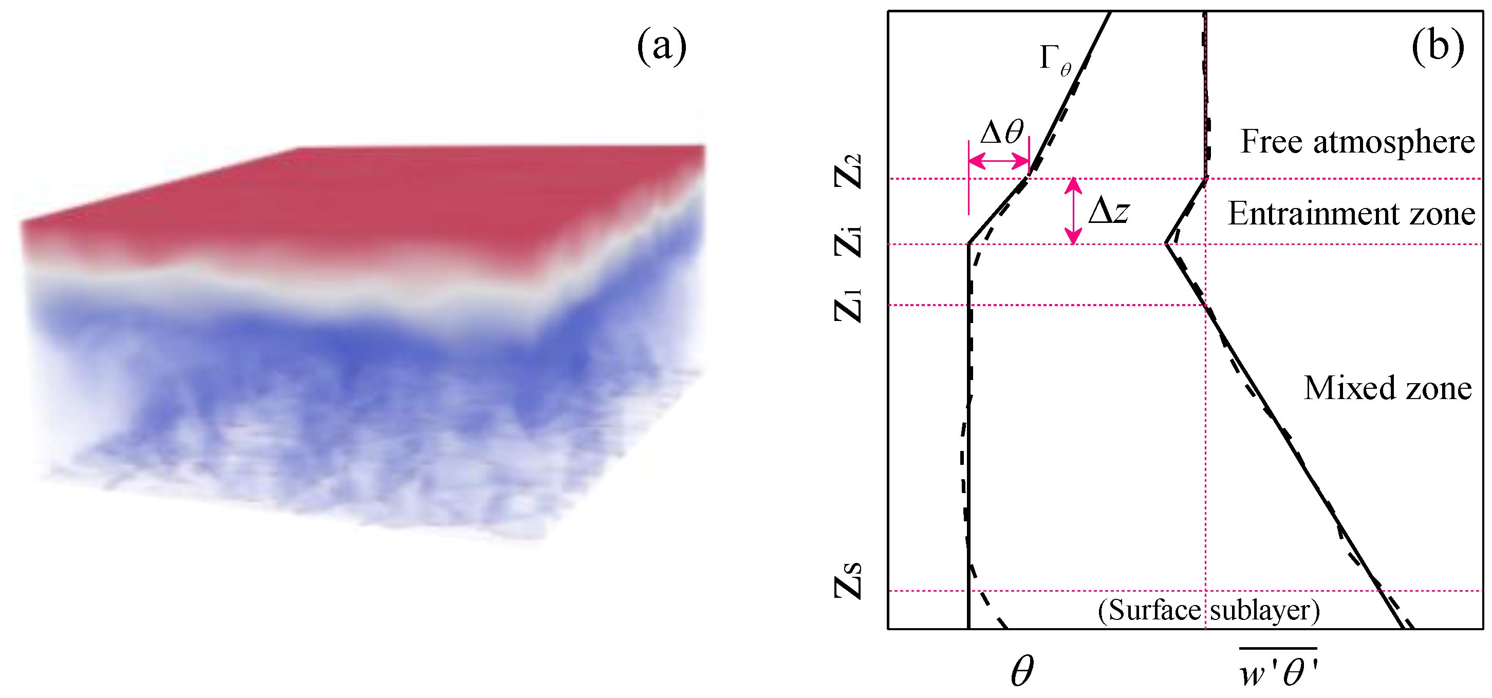
Figure 1. The schematic description of a convective boundary layer (CBL). (a) A snapshot of the thermal distribution obtained from numerical simulation and (b) the vertical profiles of the potential temperature ϴ and buoyancy flux w θ ¯ . The dashed lines represent the actual horizontally averaged profiles, and the solid lines represent their counterparts in the first-order model (FOM). Δ θ , Δ z , Γ θ and w θ | s ¯ are the potential temperature jump across the entrainment zone, the entrainment zone thickness, the gradient of the potential temperature in the free atmosphere layer, and the surface buoyancy flux, respectively. w is the vertical velocity component. The overbars denote the horizontal averages, and the primes represent the deviations from the horizontal averages.
Atmosphere 11 00063 g001
Figure 2. Evolution of the buoyancy flux profiles for the simulated cases in Table 1. The buoyancy flux is normalized by w θ ¯ | s , and the height of CBL is normalized by z i . (ai) respectively correspond to the evolution of the normalized thickness of the entrainment layer in cases when only one boundary condition ( Δ U , Γ θ and w θ ¯ | s ) is changed. The case names in the figure refer to Table 1.
Atmosphere 11 00063 g002
Figure 3. Numerically obtained Δ z / z i .plotted against the corresponding Richardson number for each of the nine models. The symbol ■ denotes the numerical data, and each straight line represents the predicted results by the corresponding model.
Atmosphere 11 00063 g003aAtmosphere 11 00063 g003b
Figure 4. (a) ln ( Δ z / z i ) plotted against ln ( R i N C 1 ) , and (b) Δ z / z i and R i N C 1 / 2 . The straight lines are the best fits to the data, and the fitted formulas are labeled at the top. The ● represents the numerical data of this paper, * represents the lidar data of Boers and Eloranta [16], □ represents the lidar data of Lothon et al. [42], and △ represents the numerical data of Otte and Wyngaard [41].
Atmosphere 11 00063 g004
Figure 5. The average distance from discrete points to the line provided by the models in Figure 3 and Figure 4.
Atmosphere 11 00063 g005
Table 1. Details of the large-eddy simulation (LES) cases with different combinations of Δ U , Γ θ and w θ ¯ | s . The first letter in the case name represents the surface buoyancy flux (A: 0.05 K·m/s, B: 0.10 K·m/s, and C: 0.15 K·m/s,), the first number after the letter denotes the extent of the potential temperature gradient (1: 0.006 K/m, 2: 0.015 K/m, and 3: 0.003 K/m), and the second number after the letter represents the velocity difference across the entrainment zone (0: 0 m/s, 1: 1.5 m/s, 2: 3.0 m/s, and 3: 4.5 m/s).
w θ ¯ | s   K · m / s Γ θ = 0.006   K / m Γ θ = 0.015   K / m Γ θ = 0.003   K / m
△U = 0 m/s△U = 1.5 m/s△U = 3 m/s△U = 4.5 m/s△U = 1.5 m/s△U = 3 m/s△U = 4.5 m/s△U = 1.5 m/s△U = 3 m/s△U = 4.5 m/s
0.05 A11A12 A21A22
0.1B10B11B12B13B21B22B23B31B32B33
0.15 C11C12 C21C22
Table 2. Typical field-observed values of the key parameters in CBL, obtained by Hibberd and Sawford [36] and their counterparts in the LES cases of the current study. Note: Pr, Re and Raf are the Prandtl number, Reynolds number, and the flux Rayleigh number, respectively. Pr = ν / α , Re = U z i / ν , and Ra f = B s z i 4 / ν D s 2 , where D s is the coefficient of diffusion.
Convective SystemU m/s Γ θ   K / m w θ ¯ | s   K   m / s z i   m w *   m / s PrRe × 108Raf × 1022
Field observation0–100.0003–0.030.03–0.3500–25000.8–3.0~0.710.3–51–7000
LES cases of this study3–7.50.003–0.0150.05–0.151000–13001.2–1.7~0.710.21–5.125–80