The 2018 Camp Fire: Meteorological Analysis Using In Situ Observations and Numerical Simulations


Abstract
1. Introduction and Background
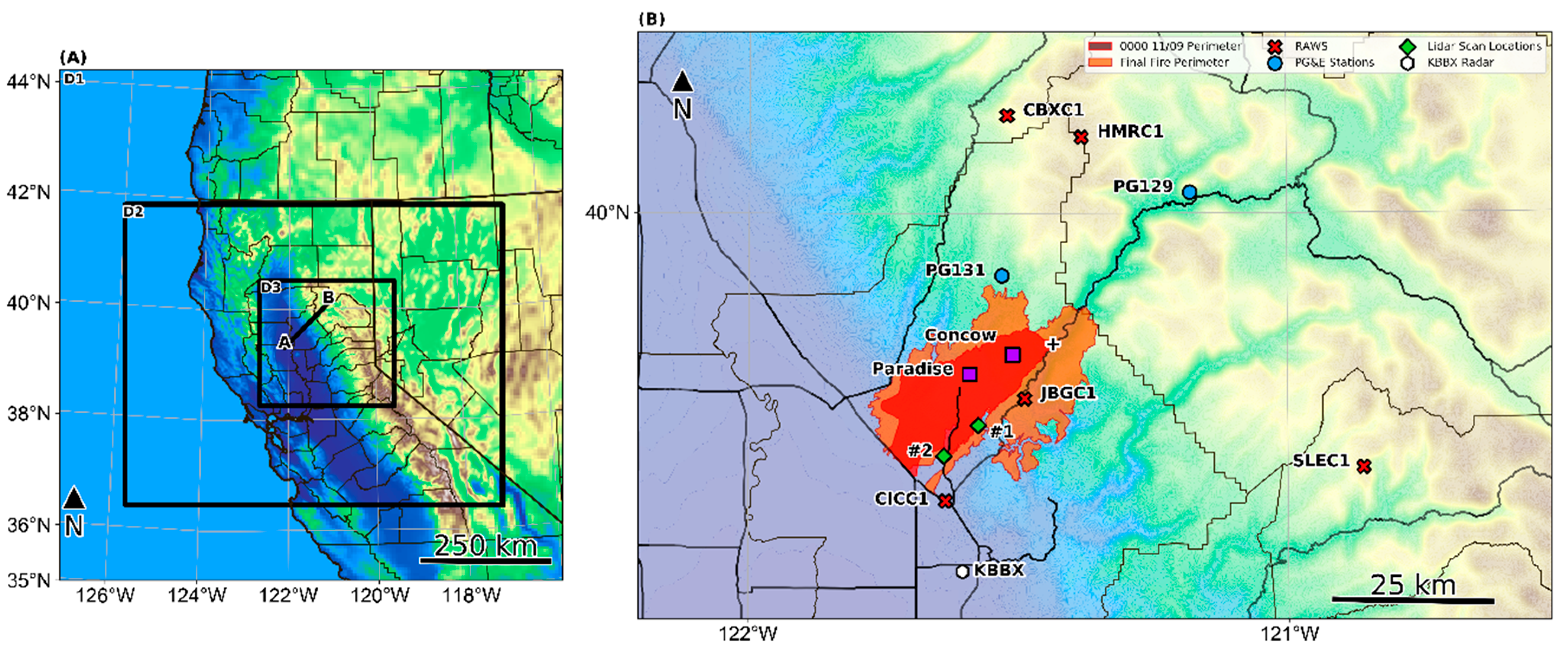
2. Data and Methodology
2.1. Observations
2.2. Modeled Data
3. Results
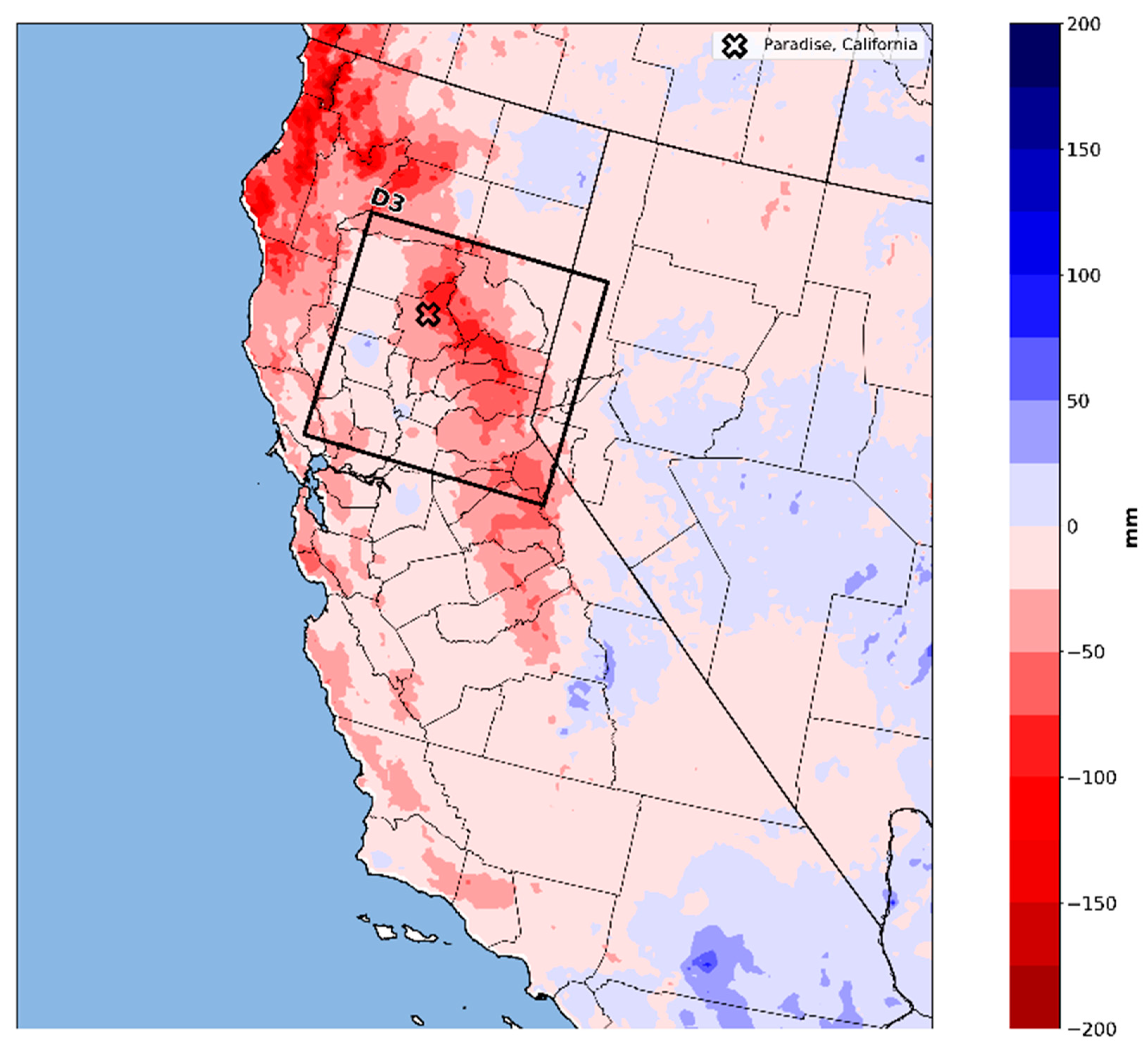
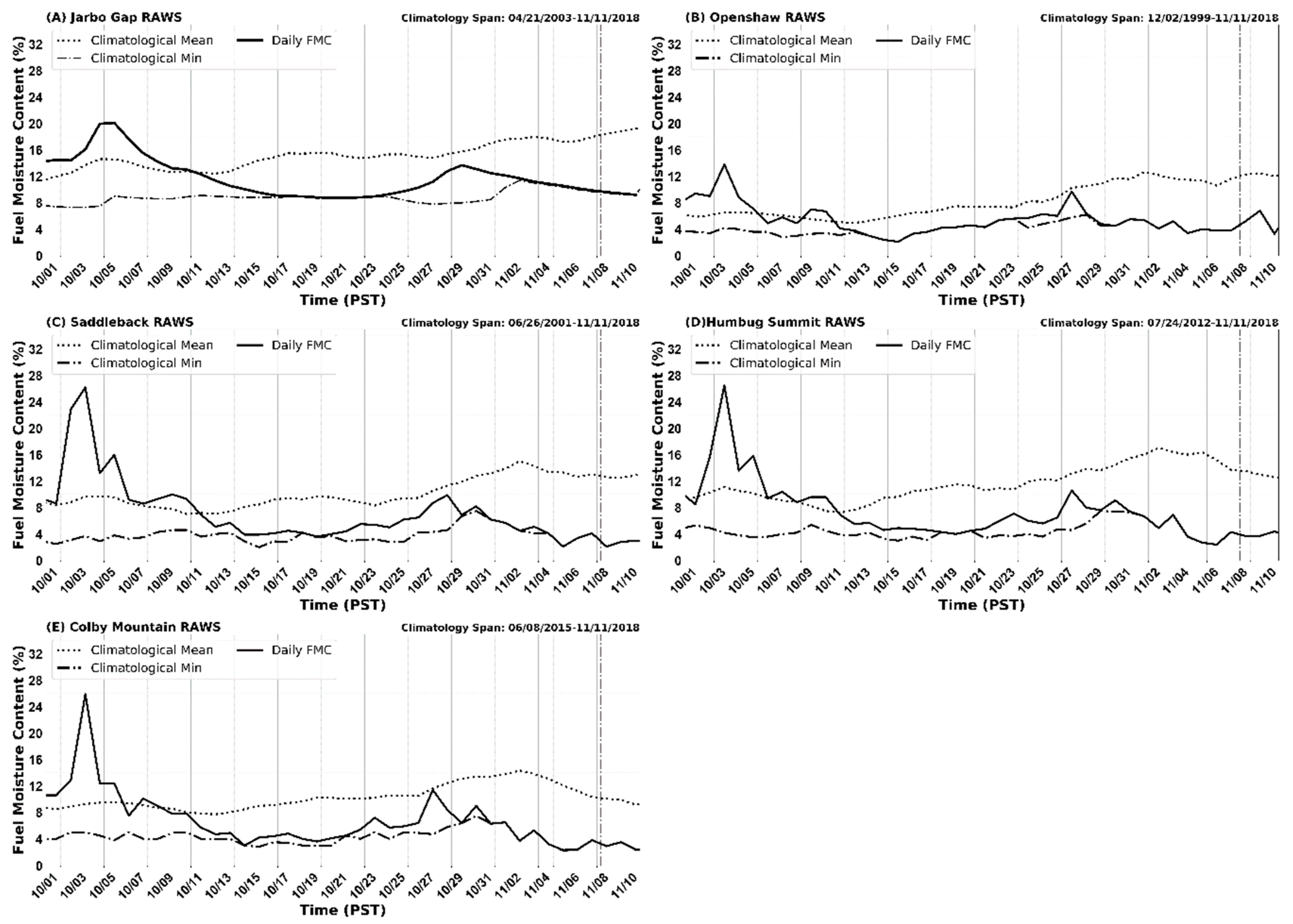
3.1. Precipitation and Fuels
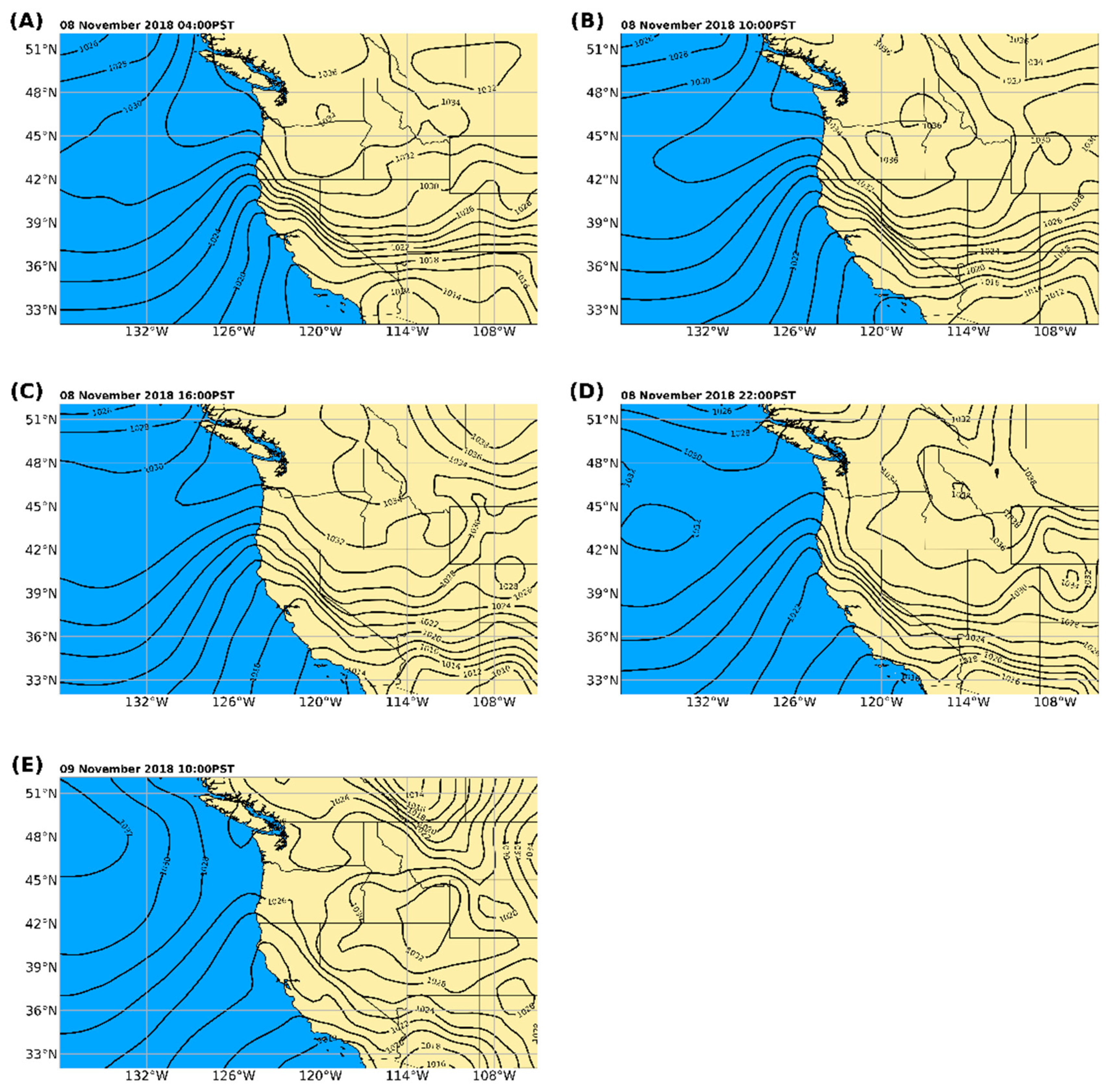
3.2. Synoptic Overview
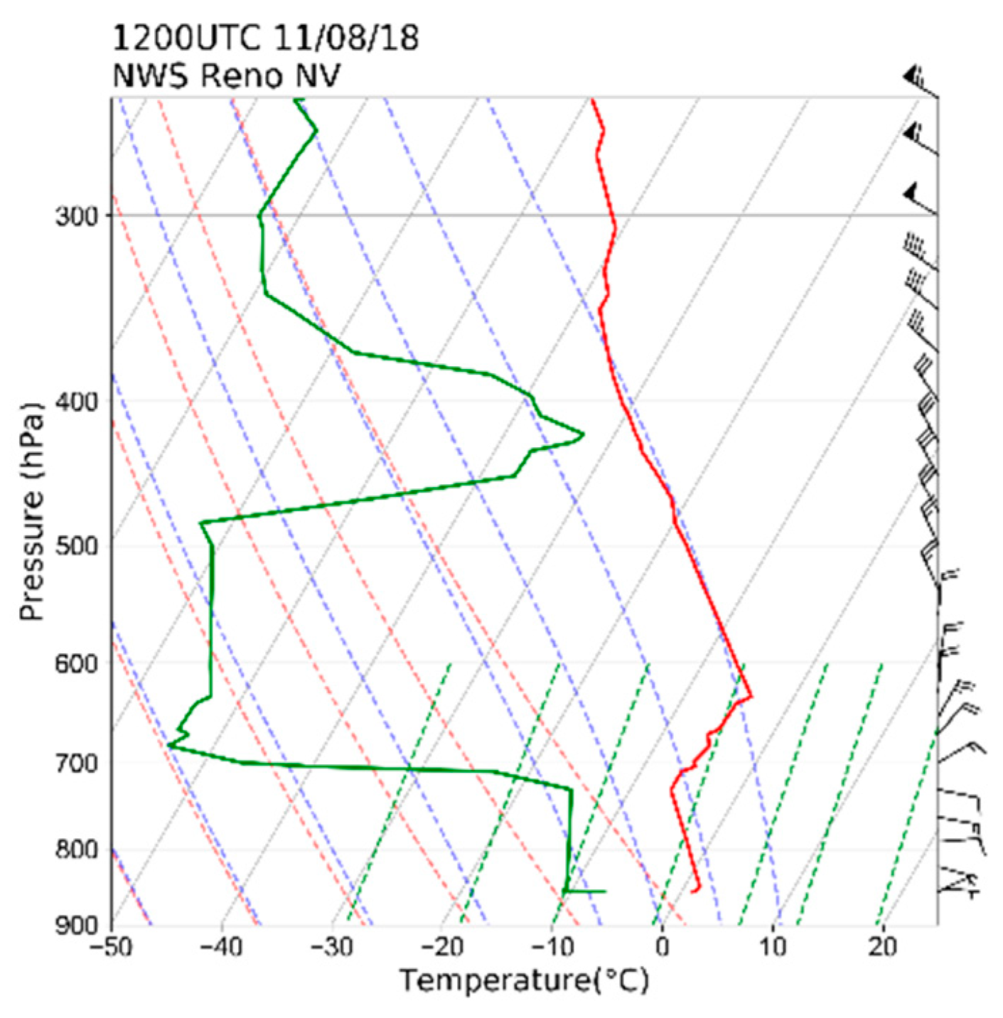
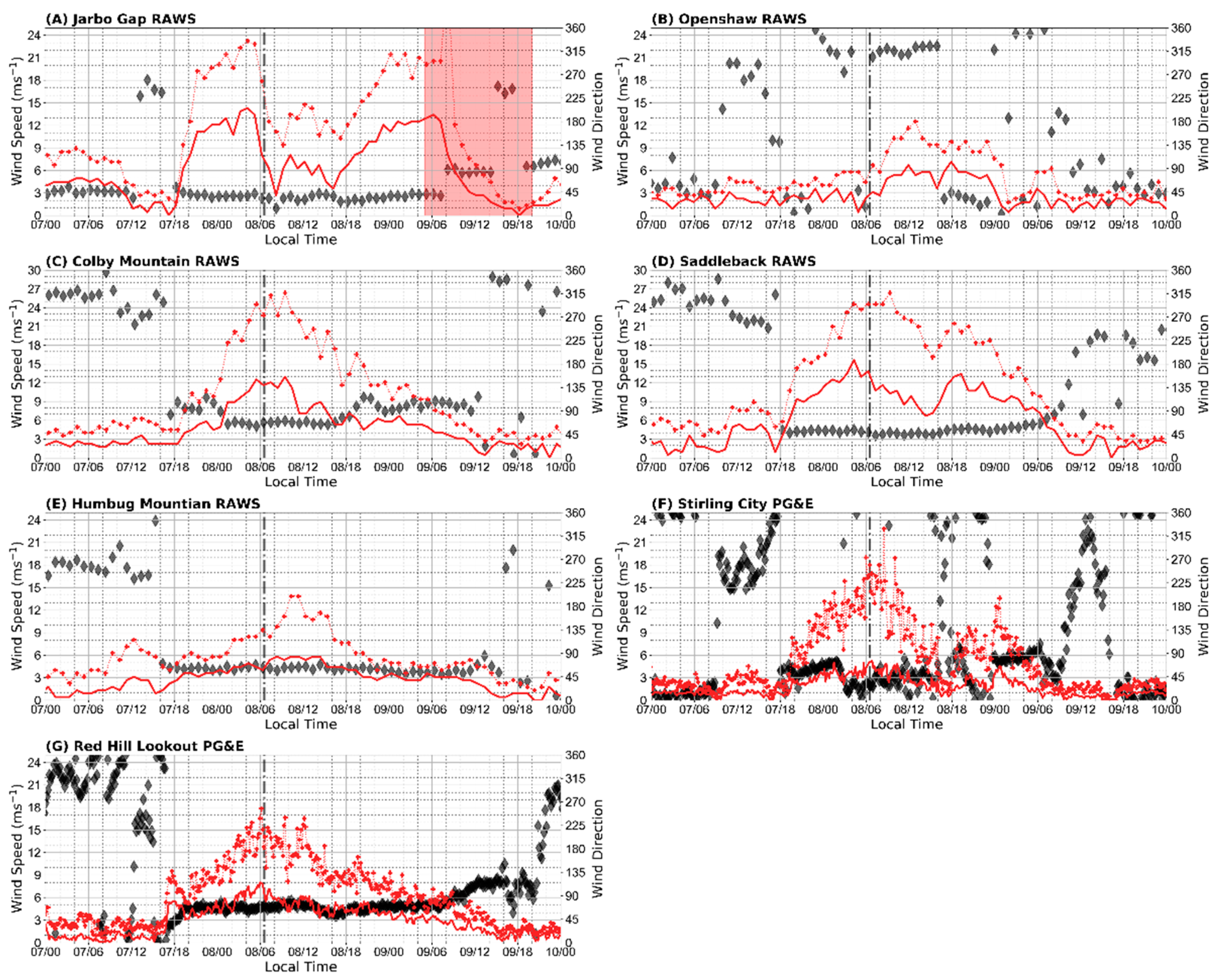
3.3. Observations
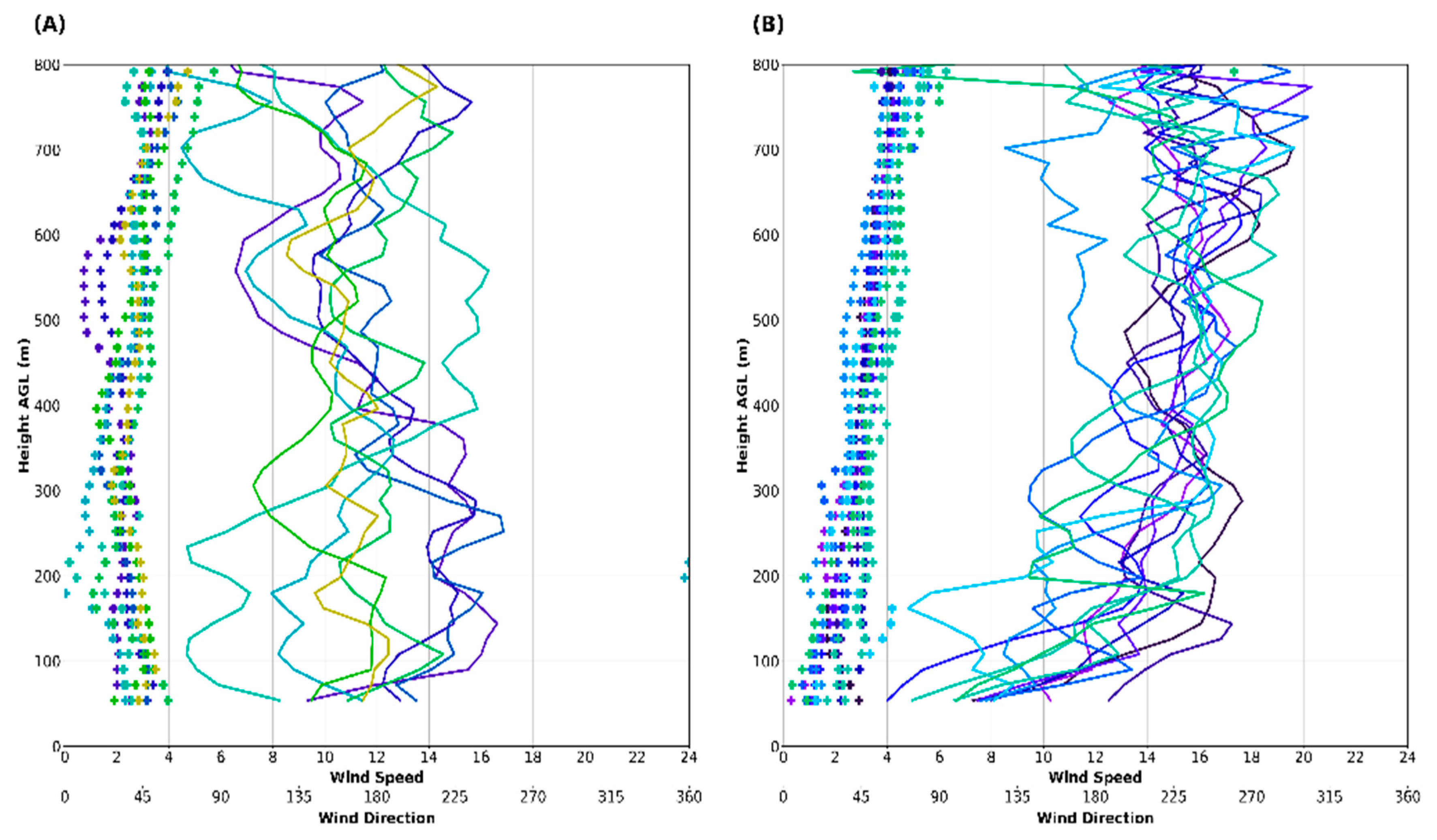
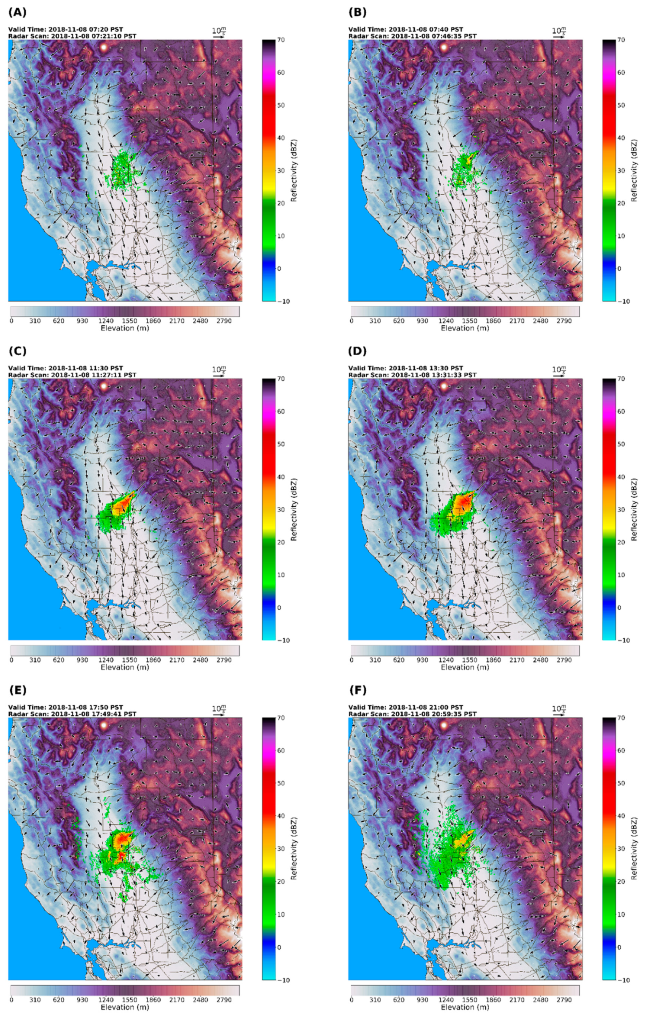
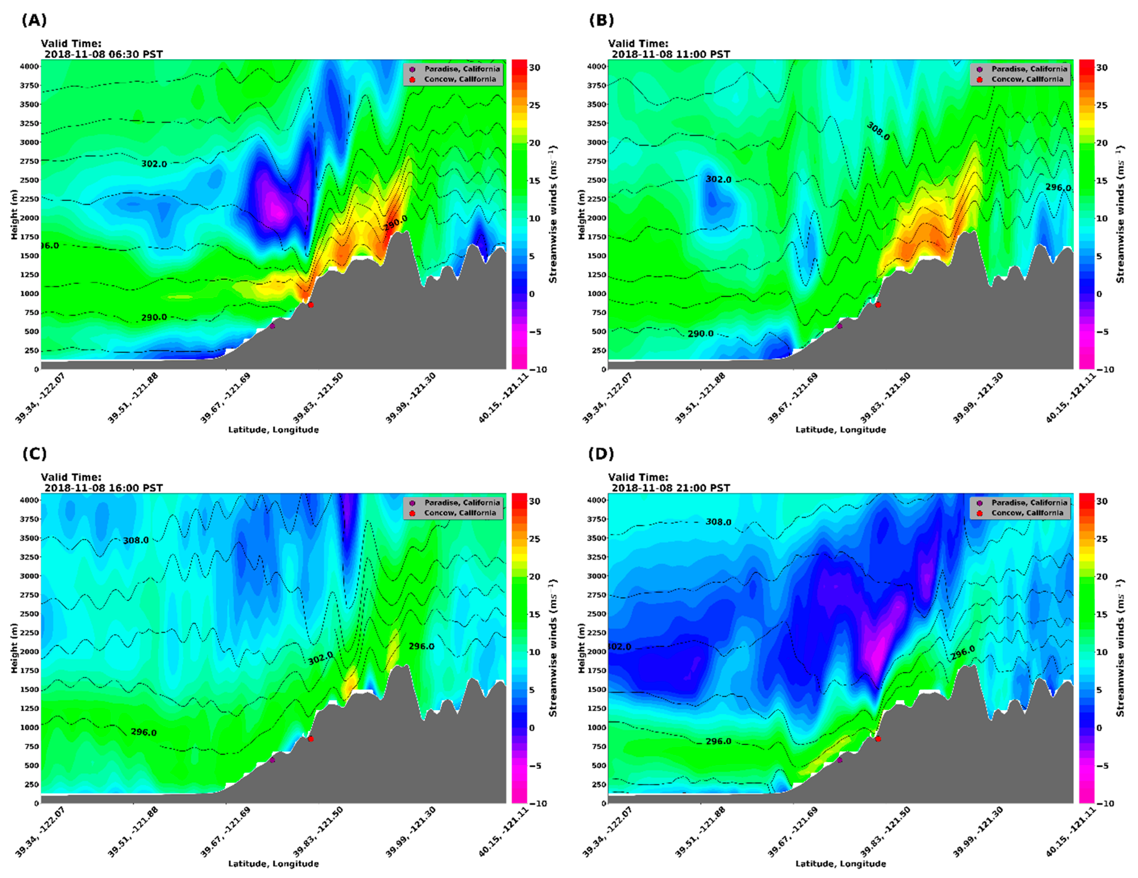
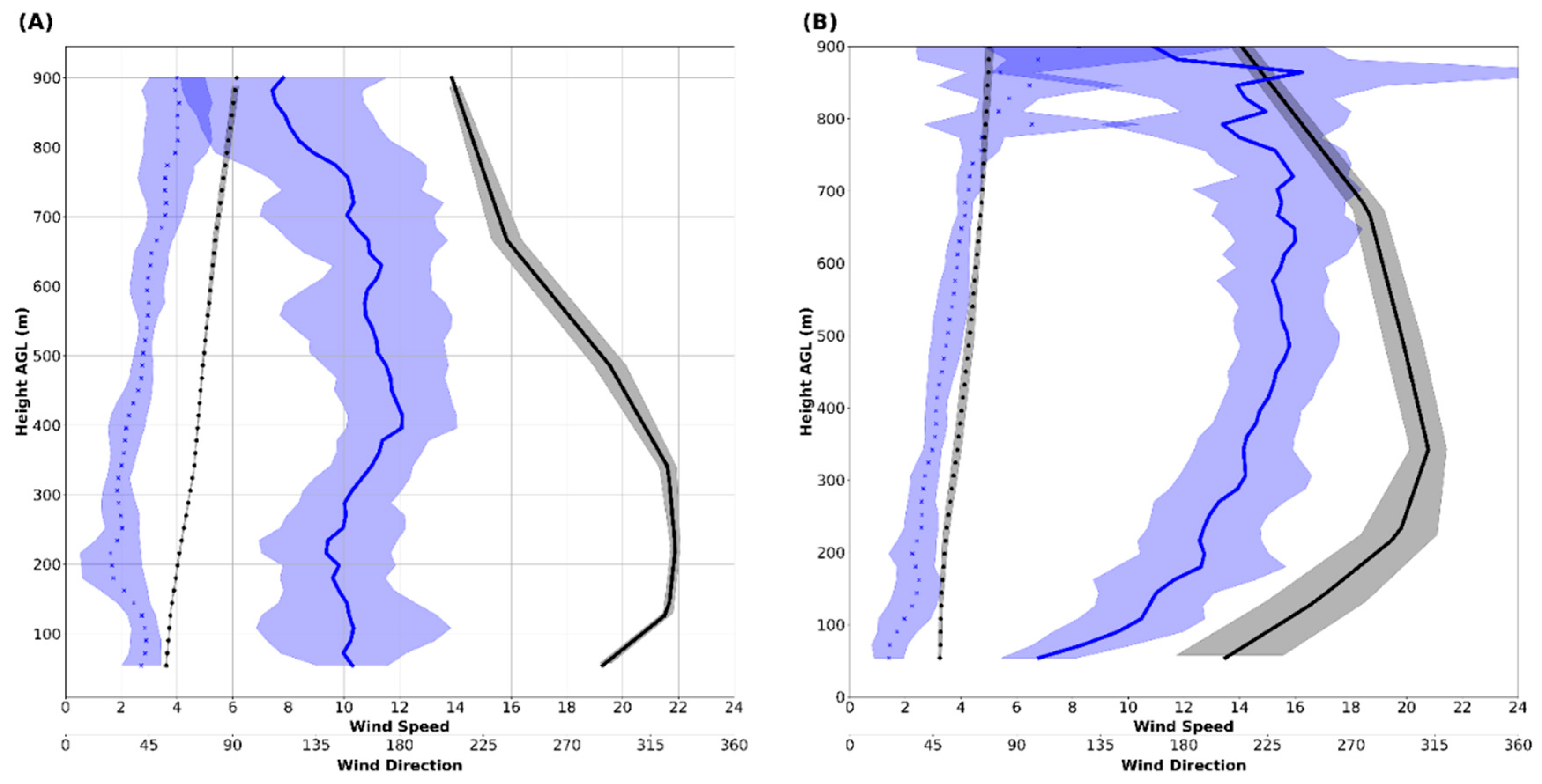
3.4. WRF Analysis
4. Model Verification
5. Discussion and Conclusions
Author Contributions
Funding
Acknowledgments
Conflicts of Interest
References
- Brinkman, W.A.R. What is a Foehn? Weather 1971, 26, 230–240. [Google Scholar] [CrossRef]
- Whiteman, C.D. Mountain Meteorology, Fundamentals and Applications; Oxford University Press: Oxford, UK; New York, NY, USA, 2000. [Google Scholar]
- Klemp, J.B.; Lilly, D.K. The Dynamics of Wave-Induced Downslope Winds. J. Atmos. Sci. 1975, 32, 320–339. [Google Scholar] [CrossRef]
- Smith, R.B. On Severe Downslope Winds. J. Atmos. Sci. 1985, 42, 2597–2603. [Google Scholar] [CrossRef]
- Durran, D.R. Mountain Waves and Downslope Winds. In Atmospheric Processes over Complex Terrain; Meteorological Monographs; Blumen, W., Ed.; American Meteorological Society: Boston, MA, USA, 1990; Volume 23, pp. 58–81. [Google Scholar] [CrossRef]
- Durran, D.R. Downslope winds. In The Encyclopedia of the Atmospheric Sciences, 1st ed.; Holton, J., Curry, J., Pyle, J., Eds.; Academic Press: Boston, MA, USA, 2004; pp. 644–650. [Google Scholar]
- Cao, Y. The Santa Ana Winds of Southern California in the Context of Fire Weather. Ph.D. Thesis, University of California, Los Angeles, CA, USA, May 2015. [Google Scholar]
- Markowski, P.; Richardson, Y. Mountain Waves and Downslope Windstorms. In Mesoscale Meteorology in Midlatitudes; Markowski, P., Richardson, Y., Eds.; John Wiley and Son: Hoboken, NJ, USA, 2010; pp. 327–348. [Google Scholar] [CrossRef]
- Westerling, A.L.; Cayan, D.R.; Brown, T.J.; Riddle, L.G. Climate, Santa Ana Winds and Autumn Wildfires in Southern California. Eos Trans. Am. Geophys. Union 2004, 85, 289–300. [Google Scholar] [CrossRef]
- Raphael, M.N. The Santa Ana Winds of California. Earth Interact. 2003, 7, 1–13. [Google Scholar] [CrossRef]
- Edinger, J.G.; Helvey, A.R.; Baumhefner, D. Surface Wind Patterns in the Los Angeles Basin during Santa Ana Conditions; Department of Meteorology, UCLA: Los Angeles, CA, USA, 1964. [Google Scholar]
- Abatzoglou, J.T.; Barbero, R.; Nauslar, N.J. Diagnosing Santa Ana Winds in Southern California with synoptic-scale analysis. Weather. Forecast. 2013, 28, 704–710. [Google Scholar] [CrossRef]
- Rolinski, T.; Capps, S.B.; Zhuang, W. Santa Ana Winds: A Descriptive Climatology. Weather. Forecast. 2019, 34, 257–275. [Google Scholar] [CrossRef]
- Cal Fire Top 20 Most Destructive California Wildfires. Available online: https://www.fire.ca.gov/stats-events/ (accessed on 5 December 2019).
- Monteverdi, J.P. The Santa Ana Weather Type and Extreme Fire Hazard in the Oakland-Berkeley Hills. Weatherwise 1973, 26, 118–121. [Google Scholar] [CrossRef]
- Bowers, C.L. The Diablo Winds of Northern California. Master’s Thesis, San Jose State University, San Jose, CA, USA, December 2018. [Google Scholar]
- Smith, C.; Hatchett, B.; Kaplan, M. A Surface Observation Based Climatology of Diablo-Like Winds in California’s Wine Country and Western Sierra Nevada. Fire 2018, 1, 25. [Google Scholar] [CrossRef]
- Werth, P.A.; Potter, B.E.; Alexander, M.E.; Clements, C.B.; Cruz, M.G.; Finney, M.A.; Forthofer, J.M.; Goodrick, S.L.; Hoffman, C.; McAllister, S.S.; et al. Synthesis of Knowledge of Extreme Fire Behavior: Volume I for Fire Managers; USDA Forest Service: Portland, OR, USA, 2011; 144p. [Google Scholar]
- Camp Fire. Available online: https://www.fire.ca.gov/incidents/2018/11/8/camp-fire/ (accessed on 20 April 2018).
- Cal Fire. Camp Incident Green Sheet; California Department of Forestry and Fire Protection: Sacramento, CA, USA, 2018.
- Cooperative Distributed Interactive Atmospheric Catalog System/Earth Observing Laboratory/National Center for Atmospheric Research/University Corporation for Atmospheric Research, and Climate Prediction Center/National Centers for Environmental Prediction/National Weather Service/NOAA/U.S. Department of Commerce. NCEP/CPC Four Kilometer Precipitation Set, Gauge and Radar; Research Data Archive at the National Center for Atmospheric Research; Computational and Information Systems Laboratory: Boulder, CO, USA, 2000. [CrossRef]
- Advanced Hydrologic Prediction Service. Available online: https://water.weather.gov/precip/download.php (accessed on 24 March 2018).
- Zachariassen, J.; Zeller, K.; Nikolov, N.; McClelland, T. A Review of the Forest Service Remote Automated Weather Station (RAWS) Network; Gen. Tech. Rep. RMRS-GTR; USDA Forest Service: Fort Collins, CO, USA, 2003; pp. 1–161. [Google Scholar]
- Cohen, J.D.; Deeming, J.E. The National Fire-Danger Rating System: Basic Equations; Gen. Tech. Rep. PSW-82; USDA Forest Service: Berkeley, CA, USA, 1985; p. 16. [Google Scholar]
- Deeming, J.E.; Burgan, R.E.; Cohen, J.D. National Fire-Danger Rating System; Dept. of Agriculture, Forest Service, Intermountain Forest and Range Experiment Station: Ogden, UT, USA, 1978. [Google Scholar]
- University of Wyoming Atmospheric Sounding. Available online: http://weather.uwyo.edu/upperair/sounding.html (accessed on 5 June 2018).
- Clements, C.B.; Oliphant, A.J. The California State University Mobile Atmospheric Profiling System: A Facility for Research and Education in Boundary Layer Meteorology. Bull. Am. Meteorol. Soc. 2014, 95, 1713–1724. [Google Scholar] [CrossRef]
- NOAA National Weather Service (NWS) Radar Operations Center. NOAA Next Generation Radar (NEXRAD) Level 2 Base Data; KBBX, NOAA National Centers for Environmental Information: Asheville, NC, USA, 1991. [CrossRef]
- Environmental Modeling Center. National Centers for Environmental Prediction; National Weather Service, NOAA, U.S. Department of Commerce: College Park, MD, USA, 2018.
- Skamarock, W.C.; Klemp, J.B.; Dudhia, J.; Gill, D.O.; Barker, D.M.; Duda, M.G.; Huang, X.Y.; Wang, W.; Powers, J.G. A Description of the Advanced Research WRF Version 3; NCAR Technical Note TN-475+ STR; National Center for Atmospheric Research: Boulder, CO, USA, 2008. [Google Scholar]
- Mesinger, F.; Kalnay, E.; Mitchell, K.; Shafran, P.C.; Ebisuzaki, W.; Jovi’c, D.; Woollen, J.; Rogers, E.; Berbery, E.H.; Ek, M.B.; et al. North American Regional Reanalysis. Bull. Am. Meteorol. Soc. 2006, 87, 343–360. [Google Scholar] [CrossRef]
- Cao, Y.; Fovell, R.G. Downslope windstorms of San Diego County. Part I: A Case Study. Mon. Weather Rev. 2016, 144, 529–552. [Google Scholar] [CrossRef]
- Cao, Y.; Fovell, R.G. Downslope Windstorms of San Diego County. Part II: Physics Ensemble Analyses and Gust Forecasting. Weather Forecast. 2018, 33, 539–559. [Google Scholar] [CrossRef]
- Fovell, R.; Gallagher, A. Winds and Gusts during the Thomas Fire. Fire 2018, 1, 47. [Google Scholar] [CrossRef]
- Pleim, J.E.; Xiu, A. Development and testing of a surface flux and planetary boundary layer model for application in mesoscale models. J. Appl. Meteorol. 1995, 34, 16–32. [Google Scholar] [CrossRef]
- Pleim, J.E. A combined local and nonlocal closure model for the atmospheric boundary layer. Part I: Model description and testing. J. Appl. Meteorol. Climatol. 2007, 46, 1383–1395. [Google Scholar] [CrossRef]
- Appenzeller, C.; Davies, H. Structure of stratospheric intrusions into the troposphere. Nature 1992, 358, 570–572. [Google Scholar] [CrossRef]
- McIntyre, M.E.; Palmer, T.N. The ‘surf zone’ in the stratosphere. J. Atmos. Terr. Phys. 1984, 46, 825–849. [Google Scholar] [CrossRef]
- McIntyre, M.E.; Palmer, T.N. Breaking planetary waves in the stratosphere. Nature 1983, 305, 593–600. [Google Scholar] [CrossRef]
- Albini, F.A. Estimating Wildfire Behavior and Effects; Gen. Tech. Rep. INT-30; USDA Forest Service: Ogden, UT, USA, 1976; p. 64. [Google Scholar]
- Cheney, N.P.; Gould, J.S. Fire Growth in Grassland Fuels. Int. J. Wildland Fire 1995, 5, 237–247. [Google Scholar] [CrossRef]


| Station Name | Station ID | Lat/Lon | Elevation (m) | Type | Record Span |
|---|---|---|---|---|---|
| Jarbo Gap | JBGC1 | 39.74, −121.49 | 773 | RAWS | 2003/04/21–Current |
| Openshaw | CICC1 | 39.59, −121.64 | 82 | RAWS | 1999/12/02–Current |
| Saddleback | SLEC1 | 39.63, −120.86 | 2033 | RAWS | 2001/06/26–Current |
| Colby Mtn. | CBXC1 | 40.14, −121.52 | 1830 | RAWS | 2015/06/08–Current |
| Humbug Summit | HMRC1 | 40.11, −121.38 | 2046 | RAWS | 2012/07/24–Current |
| Stirling City | PG131 | 39.91, −121.53 | 1143 | PG&E | 2018/10/02–Current |
| Red Hill Lookout | PG129 | 40.03, −121.18 | 1930 | PG&E | 2018/10/11–Current |
| Parameterization Type | Physics Scheme |
|---|---|
| Microphysics | Thompson graupel (8) |
| Radiation | RRTMG (4) |
| Surface layer physics | Pleim-Xiu (7) |
| Planetary Boundary Layer | ACM2 (7) |
© 2019 by the authors. Licensee MDPI, Basel, Switzerland. This article is an open access article distributed under the terms and conditions of the Creative Commons Attribution (CC BY) license (http://creativecommons.org/licenses/by/4.0/).
Share and Cite
Brewer, M.J.; Clements, C.B. The 2018 Camp Fire: Meteorological Analysis Using In Situ Observations and Numerical Simulations. Atmosphere 2020, 11, 47. https://doi.org/10.3390/atmos11010047
Brewer MJ, Clements CB. The 2018 Camp Fire: Meteorological Analysis Using In Situ Observations and Numerical Simulations. Atmosphere. 2020; 11(1):47. https://doi.org/10.3390/atmos11010047
Chicago/Turabian StyleBrewer, Matthew J., and Craig B. Clements. 2020. "The 2018 Camp Fire: Meteorological Analysis Using In Situ Observations and Numerical Simulations" Atmosphere 11, no. 1: 47. https://doi.org/10.3390/atmos11010047
APA StyleBrewer, M. J., & Clements, C. B. (2020). The 2018 Camp Fire: Meteorological Analysis Using In Situ Observations and Numerical Simulations. Atmosphere, 11(1), 47. https://doi.org/10.3390/atmos11010047