Article

Surface Aerosol Properties Studied Using a Near-Horizontal Lidar

1
Graduate School of Science and Engineering, Chiba University, 1-33 Yayoi-cho, Inage-ku, Chiba 263-8522, Japan
2
Center for Environmental Remote Sensing (CEReS), Chiba University, 1-33 Yayoi-cho, Inage-ku, Chiba 263-8522, Japan
*
Author to whom correspondence should be addressed.
Atmosphere 2020, 11(1), 36; https://doi.org/10.3390/atmos11010036
Submission received: 3 December 2019 / Revised: 20 December 2019 / Accepted: 25 December 2019 / Published: 27 December 2019
(This article belongs to the Section Aerosols)

Abstract

:
Studying near-surface aerosol properties is of importance for a better assessment of the aerosol effect on radiative forcing. We employ the data from a near-horizontal lidar to investigate the diurnal behavior of aerosol extinction and single scattering albedo (SSA) at 349 nm. The response of these parameters to ambient relative humidity (RH) is examined for the data from a one-month campaign conducted in Chiba, Japan, during November 2017, a transition period from fall to winter. The Klett method and adaptive slope method are used in deriving the aerosol extinction coefficient from the lidar data, while the SSA values are retrieved using an aethalometer. Also, a visibility-meter is used to examine the aerosol loading inside the atmospheric boundary layer. It is found that the aerosol growth during the deliquescence phase is more readily observed than the contraction in the efflorescence phase. The decrease of SSA before the deliquescence RH is found for approximately 46% of the deliquescence cases, presumably representing the particle shrinkage of soot particles.

1. Introduction

Observations of ambient aerosol optical properties near the ground are important for the Earth’s radiation budget, climate, visibility, pollution and health-related studies [1,2,3,4,5,6]. Results from these observations can also serve as ground truth data to compare aerosol products derived from satellite measurements. One of the methods to measure aerosol optical properties near the ground is the use of near-horizontal lidar operated continuously [7]. The majority of lidar studies to date have elucidated the behavior of aerosols and clouds at relatively higher altitudes (>0.5 km) [8,9,10,11]. Although continuous, near-horizontal measurements are still scarce, and this technique enables the determination of ambient optical characteristics of aerosols that are not easily observed by sampling. Most lidar systems (vertical and slant) are built and configured to have the overlap distance between the laser beam and receiver field-of-view (FOV) at a few hundred meters or more above the ground, making these systems not appropriate for near-surface aerosol studies [12,13,14,15]. A near-horizontal lidar, on the other hand, can provide information on diurnal changes of aerosols near the ground and possibly on the seasonal characterization of aerosol optical properties if operated continuously.
Compositions and optical properties of aerosols are influenced by various factors including local emission sources, advection on the regional level, long-range transport, as well as rain washout [16,17,18,19]. The present study reports the ambient aerosol behavior observed in the urban area of Chiba City, located in the southern part of the greater Tokyo metropolitan area.
Since the observation site (Chiba University) is located 3 km from the seashore along the eastern side of Tokyo Bay, the atmospheric aerosols are influenced by both urban and maritime particles. Through a long-term (seven years) sampling study conducted at Chiba University, Fukagawa et al. [20] reported that fine particles from anthropogenic emissions (such as ammonium sulfate and elemental carbon) dominate during winter, whereas coarse particles from natural origins (such as soil and sea salt) are more abundant during spring and summer. Using a stand-alone spectroradiometer, Manago et al. [21] performed measurements of skylight during the daytime under clear sky conditions and reported similar seasonal behavior of aerosol in Chiba [21]. In this paper, we describe a continuous, one-month observation using a near-horizontal lidar conducted in November 2017. This scheme enables the characterization of diurnal changes in the optical properties of ambient aerosols, even during a full-cloud cover (overcast) condition. The month of November is preferable, since it is a transition month from fall to winter, with a relatively stable atmosphere under low wind speed conditions. During the campaign period, the aerosol loading was relatively small (mostly less than 20 μg m−3), as explained below.
The influence of the ambient relative humidity (RH) on the hygroscopic aerosols has been studied in a number of previous researches [22,23,24,25,26,27,28,29], most of which were conducted using in situ sampling instruments. Single-particle measurements have elucidated how each aerosol particle having different chemical composition responds to the controlled change of RH in a chamber [30]. Studies of ambient particles with much more complex composition have usually relied on integrated nephelometers [31,32,33,34], wherein the flow rate, temperature and RH inside the instrument are controlled. However, ambiguities are unavoidable for correcting the underestimation of the aerosol scattering coefficient for factors such as the limited angular range (e.g., 7–170°) of the scattering measurement, the loss of relatively large particles due to the aerodynamic transport from the inlet pipe to the sample chamber, and the RH difference between ambient and instrumental [31,35,36]. More recently, lidars have been used to investigate the aerosol hygroscopicity, though the studies focused on higher altitudes (>500 m) [37,38,39,40]. In the present study, we characterize the properties of near-surface aerosols by means of optical instruments that are less susceptible to such corrections inherent in sampling. We employed a near-horizontal lidar to retrieve the aerosol extinction coefficient, αext, at 349 nm, together with a visibility-meter to measure αext at 550 nm. In analyzing the near-horizontal lidar data, we use the Klett method [41] with the premise of a well-mixed atmosphere, which can be validated from the range-dependence of the lidar signals. Besides, an aethalometer is used to observe the single scattering albedo, SSA, at 349 nm, in conjunction with the lidar-derived value of aerosol extinction. Although the observation of an aethalometer depends on the air sampling of the ambient atmosphere, the correction due to some loss of coarse particles (mainly due to aerodynamic transport) is considered to be of minor importance, since most of the absorptive particles (such as soot) are in the fine particle regime [42]. Ancillary instruments, such as a sunphotometer (daytime only), a vertical lidar by the National Institute for Environmental Studies (NIES; daytime and nighttime) [14,43], and a weather monitor (daytime and nighttime), are utilized to aid in categorizing the three sky conditions: clear-sky (less than 3 oktas of cloud cover), cloudy (partly cloudy to overcast, i.e., 3–5 to 8 oktas, respectively), and rainy (with intensities exceeding 15 mm/h), during the November 2017 campaign period. Here, the categorization of cloud coverage is adapted from the World Meteorological Organization (WMO) [44].
As a whole, this work aims (1) to demonstrate the capability of a near-horizontal lidar to detect the diurnal changes of aerosol optical properties near the ground, (2) to present the derived optical properties of aerosols during the change of season (November 2017, from autumn to winter) in Chiba, Japan, and (3) to characterize diurnal response of aerosol extinction coefficient with RH.

2. Weather and Aerosol Conditions in November 2017

A campaign was conducted at the Center for Environmental Remote Sensing (CEReS), Chiba University (35.63° N, 140.1° E), Chiba, Japan for the whole month of November 2017. According to the statistics of the Japan Meteorological Agency (JMA) Chiba station [45], the monthly value of total rainfall was 68.5 mm, and the mean and maximum wind speed were 3 and 8 ms−1, respectively.
Such low wind speeds indicate that the influence of soil or sea-salt particles due to strong winds was relatively small. From the data of three observation stations (operated by the local government) [46] around the current observation site, the monthly averages of PM2.5 concentrations were 12.6–13.4 μg m−3 (the maximum values of the daily mean were 21.6–23.2 μg m−3), indicating the limited aerosol loading in the lower atmosphere. The mean values of temperature and RH were 13.1 °C and 61%, respectively. The highest (lowest) temperature was 22.3 °C (2.9 °C) and the highest (lowest) RH was 96% (32%). Along with the mostly stable atmosphere, such occurrence of hot/cold as well as dry/wet conditions makes the month of November an ideal case to investigate the hygroscopic behavior of aerosol optical properties. Such a study during the seasonal transition will aid in the overall aerosol characterization that, in turn, can be used to model how aerosols affect the radiation balance in the atmosphere.

3. Instruments and Methodology

The data reported in this study are based on continuous measurements using the near-horizontal lidar [47,48], visibility-meter, aethalometer and weather monitor. Diurnal changes of near-surface aerosol parameters are analyzed and discussed at different visibility conditions, sky conditions and relative humidity (RH). Especially, the effects of RH during the deliquescence phase (increasing RH) and efflorescence phase (decreasing RH) are elucidated through the examination of αext and single scattering albedo (SSA). Since weather conditions, such as ambient temperature, wind velocity and rainfall, exert significant influence on aerosol behavior, we sorted the data into three sky conditions of clear-sky, cloudy and rainy. While the data taken during rain events are disregarded, the data before and after the rain are included in the analysis. Lidar data during rain events show the characteristics of rain rather than that of aerosols. The difference between the clear-sky and cloudy conditions is noteworthy since the insolation tends to invigorate the convection activities, resulting in the change in height of the atmospheric boundary layer. Also, the decrease in RH during the daytime is caused by solar radiation and the subsequent increase in air temperature.
Most of the instruments are located on the rooftop of an eight-story building in Chiba University, about 65 m above sea level. The campus is in the urban area of Chiba City, about 3 km away from the east side of Tokyo Bay, as shown in Figure 1. This situation makes the observation site ideal for covering the influence of both urban aerosols (predominantly from the northside and eastside of the site) and maritime aerosols (predominantly from the southside and westside of the site) during seasonal change. In the following, we will further discuss each of the instrumentation used in this study in more detail.

3.1. Near-Horizontal Lidar

The near-horizontal lidar system observes the north region to avoid direct solar radiation exposure. The elevation angle is 4°, implying that at the maximum observable range of 5 km, the equivalent altitude is approximately 350 m. Although the system is originally a plan position indicator (PPI) lidar that can perform a 360° azimuthal rotation [47,48], it was operated in a static mode during this one-month campaign period.
Figure 2 shows the schematic diagram of the lidar system, and Table 1 lists the lidar specifications. The light source is a diode-laser pumped Nd:YLF laser (Spectra-Physics, Santa Clara, CA, USA, Explorer 349) emitting at 349 nm wavelength with 60 ± 7 μJ pulse energy at 1 kHz pulse repetition rate. A photomultiplier tube (PMT, Hamamatsu Photonics, Japan, H10304-00-NN) is used as the receiver sensor in the aft-optics of a 30 cm diameter Cassegrain telescope. The PMT is connected to a transient recorder (Licel, Berlin, Germany, TR20-160) that records the backscattered signal with 5 min accumulation time at 7.5 m range resolution. The total extinction coefficient, α e x t , is derived using the Klett method [41] as
α e x t R = X R X R c α e x t R c + 2 R R c X R d R
Here, α e x t stands for the sum of aerosol (Mie) and molecular (Rayleigh) extinction within the observation range; X(R) = P(R)R2 is the range-corrected signal (RCS) derived from the background-corrected and smoothened raw signal, P(R). In the Klett analysis, careful consideration is needed to determine the appropriate value of the far-end boundary, Rc [41]. Here we define Rc from the condition that in the plot of the natural logarithm of the RCS curve against the range, a straight line (with a constant, negative slope) can reasonably be defined between the near-surface peak (RCSpeak) and RCS at Rc with a correlation factor of r2 ≥ 0.98 (see Figure 3). This condition ensures a well-mixed layer along the lidar path, and hence, the applicability of the Klett analysis.
The range corresponding to RCSpeak varies between around 400 and 800 m, representing the balance between the lidar overlap function and the effect of the aerosol profile (i.e., backscattering and extinction) along the lidar path. The resulting value of Rc, on the other hand, changes between 1.3 to 5 km on non-rainy days, and this depending on the aerosol loading. Subsequently, we employ the adaptive slope method [38] to estimate the value of α e x t (Rc).
This method relies on the premise that the atmosphere has a well-mixed aerosol layer existing below the maximum, covered altitude. Even without the effects of low-level clouds and fog, considerations are imposed for any inhomogeneous distributions, such as high aerosol loading at the far-end (e.g., from factory plumes or other sources), since this could induce uncertainties on the measured slope that may influence errors in the derived α e x t . Nevertheless, even with the uncertainties from the initial value of α e x t (Rc), the advantage of the Klett method is that the dependency of the solution on the initial estimate of the extinction coefficient at the far-end, decreases with decreasing R as discussed by Klett [41], and further verified by Matsumoto and Takeuchi [49]. Furthermore, it is noted that in Equation (1), the extinction-to-backscatter ratio (or lidar ratio, S1) is not explicitly included, though the S1 parameter is indispensable in the case of the Fernald solution [50].
Figure 3 shows the range dependence of (a) ln(RCS) and (b) the total extinction coefficient, α e x t (R), derived for the two cases of clear-sky (black line) and high aerosol loading (red line) conditions. As seen from Figure 3a, a range of around 1 or 2 km with a nearly constant slope can be found just after RCSpeak. Figure 3b shows the profiles of the total extinction coefficient calculated using Equation (1). Here our analysis focuses on the aerosol extinction coefficient at the near-surface peak, αext(RCSpeak), to obtain values as close to the surface level as possible. This implies that we assume the homogeneity in the atmospheric layer (around 30–55 m in altitude from the rooftop) between the lidar observation point and the ancillary instruments, even though the curves shown in Figure 3 exhibit non-constant behavior due to the lidar overlap function. Then, the aerosol extinction coefficient, αext(RCSpeak), is derived by subtracting the molecular contribution, n T · P z o · σ m o l e c u l e s , due to Rayleigh scattering [51]. Here, n T · P z 0 is the molecular density at the surface level under temperature T and air pressure P (at 15 °C and 1 atm, we have n T · P z 0 = 2.5469 × 1025 m−3), and σ m o l e c u l e s = 2.815 × 10⁻³⁰ cm2 is the molecular cross-section at 349 nm. It is noted that the difference between α e x t and α e x t is small, in the range of 8% to 14% of α e x t . The errors included in α e x t are due to (1) the value of α e x t (Rc), (2) the correction of Rayleigh scattering, and (3) the inhomogeneity assumption in the altitude range of 30–55 m in altitude from the rooftop where the lidar system is located. From the evaluation based on typical lidar signals, we find the error in α e x t arising from these causes is ±8%.

3.2. Visibility-Meter and Aethalometer

Meteorological optical range (MOR) data are routinely obtained every minute using a visibility-meter (present weather detector; Vaisala, Helsinki, Finland, PWD52) operated at the rooftop 4 m above the lidar system. The measurement is based on the detection of light scattered at 45° and converted to horizontal visibility, V, between 0 and 35 km. Although the scattering is measured in near-infrared (875 nm), the system automatically converts the result to the value of V at 550 nm [52]. Here the value of V represents the contribution only from the aerosol extinction, since the molecular (Rayleigh) contribution has already been removed in the conversion procedure. The accuracy of this instrument is within ±10% for 1–10 km and ±15% for 10–35 km visibility. The total extinction coefficient at 550 nm is calculated using the Koschmieder relation at the 5% contrast ratio for meteorological visibility [53] as
α e x t = ln 1 / 0.05 V
The ambient air is sampled through a 3-m vertical stainless pipe, and the aethalometer (Magee Scientific Corp., California, USA, AE31) measures the concentration of equivalent black carbon (EBC) every 5 min at seven wavelengths of 370, 470, 520, 590, 660, 880 and 950 nm with an estimated loss of less than 10% of the mass of the measured EBC [54]. These are then used to estimate the absorption coefficient α a b s as
α a b s = EBC 14625 C r e f λ
Here the coefficient Cref (= 2.14) is the correction factor of multiple scattering effects in the fiber filter employed inside the instrument [52,55,56]. A detailed discussion of the aethalometer processes and corrections is provided by Drinovec et al. [56]. The absorption coefficient, α a b s , at 349 nm is extrapolated using the power law relating the absorption coefficient and the wavelength by utilizing the Angstrom exponents from the data [57]. Then, we combine the values of α e x t R C S p e a k and α a b s to calculate the aerosol scattering coefficient, α scat = α e x t α a b s . Subsequently, the value of SSA at 349 nm is calculated [58] as
SSA = α s c a t α e x t
Although we fix the value of Cref at 2.14 in the present analysis, the choice of this coefficient affects the resulting value of SSA significantly, as discussed later in Section 4.4.
Figure 4 summarizes the flow of data in the present analysis. The near-surface aerosol optical properties ( α e x t and SSA) are derived from the data of three ground instruments, namely, the lidar, visibility-meter and aethalometer. The correlation between the α e x t from the lidar (349 nm) and the visibility-meter (550 nm) is examined, as presented below (Section 4.2). The value of SSA is calculated at 349 nm by using α e x t from the near-horizontal lidar; alternatively if α e x t from the visibility-meter were employed to calculate SSA at 550 nm, a limitation arises because of the lack of data for small aerosol loading (V ≥ 35 km). The ambient weather parameters including temperature (±0.3 °C nominal accuracy), RH (±2 percentage points), rain rate, wind speed (±1 m·s−1) and direction (±3°) are obtained every 5 min from the weather monitor (Davis Vantage Pro2).
Auxiliary instruments are also employed, such as the NIES lidar [14,43] and the sky radiometer (Prede, Tokyo, Japan, POM-02) of SKYNET [59], both of which are located inside the campus. The NIES lidar is a vertical lidar operating at the 532 and 1064 nm wavelengths using an Nd:YAG laser with the total output pulse energy of 50 mJ. It yields an aerosol profile every 15 min for altitudes higher than ~600 m with a height resolution of 30 m [14]. The sky radiometer measures the intensities of direct solar irradiance and the diffuse solar radiance distribution (315, 340, 380, 400, 500, 675, 870, 940, 1020, 1627 and 2200 nm), though its observation is limited to daytime under nearly cloudless and non-rainy conditions. One of its products is the SSA at 340 nm, as reported in the SKYNET site (http://atmos3.cr.chiba-u.jp/skynet/data.html), which is compared with the derived values of SSA at 349 nm.

4. Results and Discussion

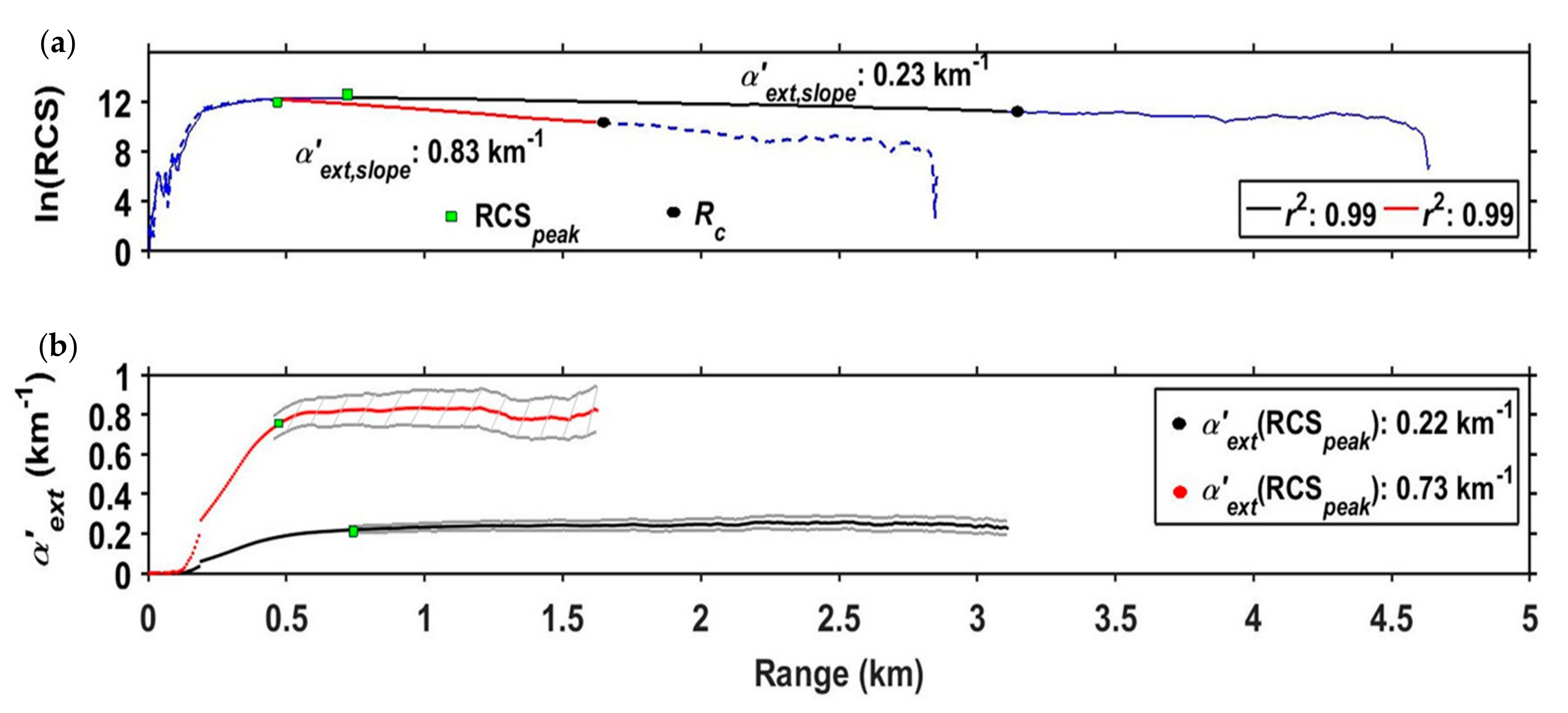
4.1. Lidar-Derived Total Extinction Coefficient

Figure 5 shows the temporal change of (a) the lidar signal intensity represented by the RCSpeak in the natural logarithm scale, (b) the lidar-derived total extinction coefficient, α e x t and (c) the rain rate during the one-month observation period. In Figure 5a, decrease in the signal intensity is observed during the time of rain: also, decrease in the lidar peak height occurs for the cases of high aerosol loading, namely, during 2, 6–7, 9, 20, 26 and 28–29 November, as enclosed in red broken lines in Figure 5a. In these cases, the lidar-derived total extinction, α e x t , often exhibits high values (>0.6 km−1). As a consequence, the range that corresponds to RCSpeak is not constant in the one-month observation, but, varies between around 400 and 800 m, which represents the altitude range between ~30 and ~55 m with respect to the lidar system elevation (about 65 m above the sea level). Moreover, the effect of rain (wet deposition) can clearly be observed in the temporal change of α e x t in Figure 5b (i.e., 3, 4, 8, 11, 13–15, 22–24 and 30 November). The total extinction profile in Figure 5b shows that the atmosphere below Rc (the far-end optical range in Figure 5b) is fairly well mixed in the entire campaign.

4.2. Correlation between Lidar and Visibility-Meter Data

Figure 6 shows the scatter plot between the aerosol extinction, αext, at 550 nm derived from the visibility-meter and αext at 349 nm derived from the near-horizontal lidar signals. Figure 6a (with 5529 points) shows all the data points (every 5 min) during the one-month campaign, except those in rain events (i.e., data during the moment of rain were excluded), while Figure 6b (3006 points) shows the data for no-rain days (i.e., 17 days without a rain out of the 28 day-data). The r2 values are based on the least absolute residuals (LAR) regression analysis [60]. A closer examination of the points indicates that in both Figure 6a,b, the outliers are from the data just after rain events, presumably due to the droplets forming on the glass window on the lidar path. An improved correlation coefficient (r2 = 0.98) results when the outliers are excluded, as shown in Figure 6b. This relation can be used to extrapolate the values of visibility (and hence, the extinction coefficient) when the visibility exceeds 35 km (i.e., low aerosol loading); the possible error range due to this extrapolation is ±6%.
Moreover, from the regression line and the scattered data points in Figure 6b, the Angstrom exponent (AE) between 349 and 550 nm is estimated to be 2.0 ± 0.5. Fukagawa et al. [20] reported that during midday (10:00 and 14:00 JST) under a clear-sky condition in Chiba, the value of AE is in the range of 1.2 to 1.8 during October and February from the data (at 368, 500, 675 and 778 nm) of the sunphotometer and sky radiometer (SKYNET) observed between the years 2000 and 2005. Also, Manago et al. [21] reported the same range of AE for clear-sky conditions in Chiba from spectroradiometer observations (350–1050 nm with 10 nm resolution) of direct and scattered solar radiation conducted in 2007 and 2008. From our current data, we select specific days (e.g., 5, 12 and 21 November) with clear-sky conditions; the derived AE is from 1.2 to 2.0, in agreement with the values from our previous works [20,21]. The comparison between the current results and SKYNET SSA will be given below (Section 4.4).

4.3. Relation of Near-Surface αext to Atmospheric Boundary Layer Height

Most aerosol particles reside inside the atmospheric boundary layer [24]. Its height (boundary layer height, BLH) is affected by the insolation, temperature gradient, moisture and wind (due to air mass transfer). Thus, the daytime BLH is generally higher than the nighttime BLH. An increasing BLH implies a higher possibility of aerosol convection process, and this decreases aerosol concentration near the surface when the wind-driven advection effect is insignificant [61]. During the low BLH condition, on the other hand, the influence of atmospheric convection is reduced. During November in Chiba, the formation of a nocturnal inversion layer sometimes occurs during nighttime without cloud coverage.
From the RCS of the NIES-lidar data (532 nm) with a full-overlap range at ~600 m [14], the BLH values can be estimated using the cubic root gradient method proposed by Yang et al. [62] as
BLH = R C S 1 / 3 R
Here, BLH corresponds to the altitude where the cubic root RCS gradient reaches a minimum. The derived BLHs exhibit root mean square errors (RMSEs) of 120–140 m [62]. Although Yang et al. [53] clearly identified the nocturnal boundary layer in one-diurnal cycle and compared it to radiosonde and three common gradient methods (i.e., first gradient method, first logarithm gradient method, and first normalized gradient method), our result is limited to identifying BLH ≥ 600 m due to the NIES-lidar overlap limitation.
Figure 7 shows the relation between the near surface value of αext (at 349 nm) and BLH during non-rainy days. For this purpose, the values of αext from the near-horizontal lidar have been averaged every 15 min to be comparable with the NIES lidar acquisition rate. From this figure, it is found that the functional relation between the aerosol extinction coefficient αext, and BLH, follows a power–law decay to a first order approximation with a correlation value of r2 = 0.99 with RMSE = 0.0064. This implies that the aerosol concentration tends to be controlled by the change in the BLH except for the days with rain and some cases with relatively high wind speeds (≥3 m·s−1). Among a total of 430 points plotted in Figure 7, we have 57 points (13%) with high wind speed events. However, it is noted that during nighttime, Equation (5) often detects the residual layer (i.e., the elevated remnants of the convective boundary layer in the previous daytime) instead of the BLH that corresponds to the nocturnal boundary layer itself. Thus, the correlation found in Figure 7 can be underestimated to some extent, and this is partly ascribed to the limitation due to the overlap of the NIES lidar (600 m).

4.4. One-Month Variations of αext and SSA

Figure 8 shows the temporal variations of (a) visibility condition, (b) αext from both the lidar and visibility-meter data, (c) SSA from the lidar and sky radiometer of SKYNET, (d) RH/ambient temperature, (e) rain rate, (f) wind direction and (g) wind speed over the whole campaign period of November 2017. In Figure 8a,b, the red lines in the visibility-meter data denote the extrapolation to V ≥ 35 km using the result shown in Figure 6b. In Figure 8b, the systematic difference between the two curves (blue, near-horizontal lidar; black and red, visibility-meter) arises from the difference in the observation wavelengths (349 and 550 nm, respectively). Figure 8c shows the comparison of SSA between the lidar/aethalometer and sky radiometer data. In analyzing the aethalometer data, we have employed a correction coefficient Cref = 2.14 (Equation (3)). The mean and standard deviation (SD, 1σ) of SSA is 0.93 and 0.04, respectively, for the whole period of 28 days. When the value of Cref is changed to 1.0 (i.e., no correction of fiber scattering) or 3.5 (a value proposed in a previous research [63]), the resulting values of the mean and SD are (0.86, 0.09) and (0.96, 0.02), respectively.
The mean and SD of sky radiometer data are 0.89 and 0.05, which suggests that the present choice of Cref = 2.14 is reasonable. The sky radiometer values are somewhat smaller (i.e., more absorptive): this is probably due to the wider range of observation altitudes (up to free troposphere) of the sky radiometer. Most (96%) of the values of SSA from the lidar and aethalometer measurements are in the range from 0.85 to 1, occasionally showing minima during the nighttime. The sky radiometer values, on the other hand, tend to exhibit minimum values as small as 0.76 during the daytime. A possible cause of this discrepancy between the two methods is the formation of nocturnal boundary layers, and hence, the change in the BLH, as indicated in Figure 7. During winter in Chiba, the volume concentration of elemental carbon is about 22.7%, as reported by Fukagawa et al. [20]. Thus, the temporal change of aerosol vertical profile along with BLH might lead to the change in SSA between the near-surface and upper atmosphere, though more detailed studies are needed to elucidate the vertical profile of SSA.
As seen from Figure 8d, both the ambient temperature and RH exhibit diurnal changes: low and high values of RH are observed in midday and nighttime, respectively. The limited extent of the rain (Figure 8e) during the observation period infers the low influence of aerosol washout. Besides, the low wind speed (less than 4 m·s−1 for 95% of the time) for most of the days (except 8–9, 11, 18 and 26 November) suggests that the effect of advection was insignificant.
Therefore, given the diurnal pattern of RH (Figure 8d), it is possible to evaluate the influence of RH on aerosol characteristics, namely, the onset of deliquescence (size growth) with increasing RH as well as that of efflorescence (drying out) with decreasing RH. Generally, the value of αext is expected to increase or decrease with such changes of RH [64,65]. In the present measurement, the wind direction is another factor that affects the aerosol optical property because of the location of our observation site near Tokyo Bay (Figure 1). Figure 8f indicates that wind was blowing predominantly from the north or east direction (77% of the time), and hence, the particles are mostly from the urban area of Chiba City. For cases with relatively stronger wind speed (≥4 m·s−1), on the other hand, the wind direction was predominantly from the south or west, resulting in the transportation of marine aerosols from Tokyo Bay. The formation of the nocturnal boundary layer and the subsequent increase in the BLH due to the insolation also affect the aerosol concentration in the lowest part of the troposphere [17,66,67,68]. Below, we will discuss how the values of αext and SSA are affected by various meteorological parameters by considering three different sky conditions: clear (i.e., insolation in the daytime), cloudy (stable atmosphere) and rainy.

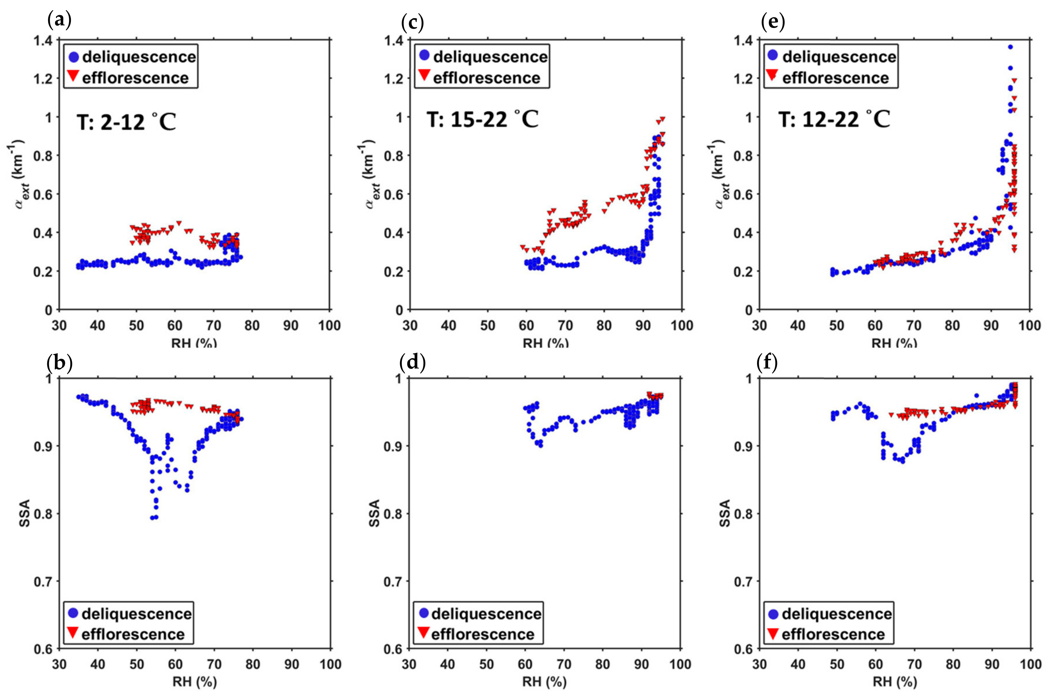
4.5. Influence of Varying Sky Conditions and RH on Near-Surface αext and SSA

Hygroscopic aerosols (e.g., ammonium nitrate, ammonium sulfate and sodium chloride) exhibit hysteresis behavior during the increase and subsequent decrease of RH [69]. Figure 9 shows a 24-h diurnal variation of αext and SSA and their corresponding hysteresis (complete and incomplete) curves with RH measured during the deliquescence phase (from the midday minimum RH to late evening high RH), and the efflorescence phase (from the late evening high RH to midday minimum RH of the next day) for clear ((a) and (b), 21–22 November), cloudy ((c)–(d), 3–4 November) and rainy ((e)–(f), 2–3 November) conditions. Here, we discuss the influence of RH for a cycle of afternoon–night–morning, since the lack of insolation during the nighttime infers a more stable condition of the lower troposphere, as compared with daytime. For these days, the wind speed was less than 3 m·s−1 and the wind came predominantly from the N-NE direction (urban aerosols), with occasional occurrence of S-SW direction (maritime aerosol). From Figure 9c,e during the deliquescence phase (blue dots), the curve patterns of αext are comparable to the humidograph of a hygroscopic aerosol [69]. As RH increases (clear-sky: 35% < RH < 74%, cloudy: 60% < RH < 73% and rainy: 49% < RH < 71%), the value of αext is almost stable, and right after the deliquescence humidity (clear-sky: 74%, cloudy: 73% and rainy: 71%), the rapid increase in αext is apparent. The cases of the efflorescence phase (red triangles), on the other hand, are seen typically around early dawn to midday in a temperature range of about 2–22 °C. Although a complete hysteresis curve is observed under the cloudy condition, this is not the case for clear and rainy conditions. This can be ascribed to either the incomplete deliquescence–efflorescence cycle in a day to reach the efflorescence RH, or rapid increase in the BLH.
Among a total of 28 cases (days) of deliquescence–efflorescence cycles within the whole campaign period, 11 days were observed to have the hygroscopic growth pattern (clear-sky: 2, cloudy: 5, rainy: 4). For the efflorescence phase, on the other hand, only four days (cloudy: 3, rainy: 1) were observed to have a complete hysteresis (reaching the efflorescence RH) and seven days (clear: 3, cloudy: 2, rainy: 2) with incomplete hysteresis (not reaching the efflorescence RH).
Figure 9b,d,f show examples of the relationship observed between SSA and RH. There is an apparent decrease in SSA during the deliquescence phase just before the deliquescence RH (clear-sky: 35% < RH < 63%, cloudy: 60% < RH < 73% and rainy: 49% < RH < 67%), then the value increases again after the deliquescence RH. This occurs in 13 cases out of the 28-day deliquescence–efflorescence cycles (46%). Closer inspection has revealed that the decrease of SSA value before the deliquescence RH is mainly due to the increase in the EBC count of the aethalometer (clear-sky: 2430 ng·m−3, cloudy: 668 ng·m−3 and rainy: 1424 ng·m−3). However, it also coincides with the slight decrease in αext before the deliquescence RH (8 out of 13 cases), which is referred to as the “particle shrinkage” effect that is due to particle structural rearrangement [70,71,72,73]. From laboratory data using a tandem differential mobility analyzer, for instance, Weingartner et al. [73,74] reported such structural changes of combustion aerosol particles with increasing RH.
They indicated that this shrinking effect is attributed to the capillary forces induced on any asymmetric part of the particles that caused them to become a more compact structure, and is more pronounced in larger particles with diameters exceeding 50 nm [73].

5. Conclusions

We have described a set of the methodology used to estimate the near-surface aerosol optical properties, namely, the aerosol extinction coefficient (αext) and SSA, using a near-horizontal lidar, a visibility-meter and an aethalometer. The analysis of one-month data has revealed the sensitivity of the lidar return signals to both aerosol loading and sky conditions. The examination of the range-corrected lidar signals has revealed the applicability of the Klett method in deriving the total extinction coefficient, α e x t R . Despite the uncertainty in the determination of the far-end boundary value, α e x t R c , the resulting values of αext(RCSpeak) exhibit a reasonable correlation with αext derived from the visibility-meter (non-rainy days) with an LAR r2 value of 0.98. From the lidar (349 nm) and visibility-meter (550 nm) data, the value of AE has been estimated to be 1.2 to 2.0 under clear-sky conditions, in agreement with the values reported in other investigations conducted in Chiba. The effects of meteorological parameters to the derived aerosol optical properties have also been considered. The wind speed was relatively low (<4 m·s−1 for 95% of the time), suggesting that the wind-driven advection is insignificant. This could explain the power–law relation (negative correlation) observed between αext from lidar (349 nm) and BLH from the NIES lidar (532 nm), to a first-order approximation, for BLH exceeding 600 m. With the appropriate choice of the correction factor (Cref = 2.14) for the aethalometer data, it is found that the resulting values of SSA are similar to those from the sky radiometer data, though the latter exhibit some influence of the atmosphere above the BLH.
We have conducted the ambient investigation of the hygroscopicity of aerosols by exploiting the diurnal variability in the transition month of November when the atmospheric conditions are mostly calm. Hygroscopic growth characteristics are observed for 11 days during the campaign period (a total of 28-day deliquescence–efflorescence cycles), whereas the occurrence of hysteresis during the efflorescence phase has been observed for four days (complete hysteresis—reaching the efflorescence RH), and seven days (incomplete hysteresis). The fluctuation of SSA during the deliquescence phase was observed to coincide with the small fluctuation in αext before the deliquescence RH. This variation in αext has been found in 13 cases (46%) out of the 28-day deliquescence–efflorescence cycles, indicating the possible occurrence of the aerosol shrinkage.
In conclusion, we have demonstrated the capability of a near-horizontal lidar to detect diurnal changes of aerosol optical properties near the ground and to characterize the diurnal response of aerosol extinction coefficient with RH. The future extension of the present work will include the application of the reported method to other seasons and other locations.

Author Contributions

Methodology, P.M.O.; formal analysis, P.M.O.; resources, H.K.; data curation, P.M.O., N.L.; writing—original draft preparation, P.M.O.; writing—review and editing, N.L., H.K.; supervision, H.K., T.S. All authors have read and agreed to the published version of the manuscript.

Funding

This research received no external funding.

Acknowledgments

The authors would like to thank H. Irie and T. Takamura for their efforts in maintaining the SKYNET sites, with promoting the use of their data and products. Also, we are grateful to the NIES lidar team for providing us with the data required for estimating the boundary layer height. The first author (P.M.O.) would also like to thank the Ministry of Education, Culture, Sports, Science and Technology (MEXT) of Japan through the Monbukagakusho scholarship that supports her research activity and education in Chiba University.

Conflicts of Interest

The authors declare no conflict of interest.

References

  1. Climate Change 2013—The Physical Science Basis. Contribution of Working Group I to the Fifth Assessment Report of the Intergovernmental Panel on Climate Change; Cambridge University Press: New York, NY, USA, 2013; pp. 33–118. [Google Scholar]
  2. Hobbs, P.V. Aerosol-cloud interactions. In International Geophysics; Elsevier: Amsterdam, The Netherlands, 1993; Volume 54, pp. 33–73. [Google Scholar]
  3. Seinfeld, J.H.; Pandis, S.N. Atmospheric Chemistry and Physics: From Air Pollution to Climate Change; John Wiley & Sons: Hoboken, NJ, USA, 2016. [Google Scholar]
  4. Abbey, D.E.; Nishino, N.; McDonnell, W.F.; Burchette, R.J.; Knutsen, S.F.; Lawrence Beeson, W.; Yang, J.X. Long-term inhalable particles and other air pollutants related to mortality in nonsmokers. Am. J. Respir. Crit. Care Med. 1999, 159, 373–382. [Google Scholar] [CrossRef] [PubMed] [Green Version]
  5. Pope, C.A., III; Burnett, R.T.; Thun, M.J.; Calle, E.E.; Krewski, D.; Ito, K.; Thurston, G.D. Lung cancer, cardiopulmonary mortality, and long-term exposure to fine particulate air pollution. JAMA 2002, 287, 1132–1141. [Google Scholar] [CrossRef] [PubMed] [Green Version]
  6. Samet, J.M.; Dominici, F.; Curriero, F.C.; Coursac, I.; Zeger, S.L. Fine particulate air pollution and mortality in 20 US cities, 1987–1994. N. Engl. J. Med. 2000, 343, 1742–1749. [Google Scholar] [CrossRef] [PubMed]
  7. Dreischuh, T.; Grigorov, I.; Peshev, Z.; Deleva, A.; Kolarov, G.; Stoyanov, D. Lidar Mapping of Near-Surface Aerosol Fields. Aerosols-Sci. Case Stud. 2016, 85–107. [Google Scholar] [CrossRef] [Green Version]
  8. Maki, T.; Furumoto, S.; Asahi, Y.; Lee, K.C.; Watanabe, K.; Aoki, K.; Murakami, M.; Tajiri, T.; Hasegawa, H.; Mashio, A. Long-range-transported bioaerosols captured in snow cover on Mount Tateyama, Japan: Impacts of Asian-dust events on airborne bacterial dynamics relating to ice-nucleation activities. Atmos. Chem. Phys. 2018, 18, 8155–8171. [Google Scholar] [CrossRef] [Green Version]
  9. Nishizawa, T.; Sugimoto, N.; Matsui, I.; Shimizu, A.; Hara, Y.; Itsushi, U.; Yasunaga, K.; Kudo, R.; Kim, S.-W. Ground-based network observation using Mie–Raman lidars and multi-wavelength Raman lidars and algorithm to retrieve distributions of aerosol components. J. Quant. Spectrosc. Radiat. Transf. 2017, 188, 79–93. [Google Scholar] [CrossRef]
  10. Tsedendamba, P.; Dulam, J.; Baba, K.; Hagiwara, K.; Noda, J.; Kawai, K.; Sumiya, G.; McCarthy, C.; Kai, K.; Hoshino, B. Northeast asian dust transport: A case study of a dust storm event from 28 March to 2 April 2012. Atmosphere 2019, 10, 69. [Google Scholar] [CrossRef] [Green Version]
  11. Vaughan, M.A.; Powell, K.A.; Winker, D.M.; Hostetler, C.A.; Kuehn, R.E.; Hunt, W.H.; Getzewich, B.J.; Young, S.A.; Liu, Z.; McGill, M.J. Fully automated detection of cloud and aerosol layers in the CALIPSO lidar measurements. J. Atmos. Ocean. Technol. 2009, 26, 2034–2050. [Google Scholar] [CrossRef]
  12. Sasano, Y.; Shimizu, H.; Takeuchi, N.; Okuda, M. Geometrical form factor in the laser radar equation: An experimental determination. Appl. Opt. 1979, 18, 3908–3910. [Google Scholar] [CrossRef]
  13. Wandinger, U.; Ansmann, A. Experimental determination of the lidar overlap profile with Raman lidar. Appl. Opt. 2002, 41, 511–514. [Google Scholar] [CrossRef]
  14. Shimizu, A.; Sugimoto, N.; Matsui, I. Detailed description of data processing system for lidar network in East Asia. In Proceedings of the 25th International Laser Radar Conference, St. Petersburg, Russia, 5–9 July 2010; pp. 911–913. [Google Scholar]
  15. Satheesh, S.; Vinoj, V.; Moorthy, K.K. Vertical distribution of aerosols over an urban continental site in India inferred using a micro pulse lidar. Geophys. Res. Lett. 2006, 33. [Google Scholar] [CrossRef]
  16. Takahashi, K. Long-Term Variation of Atmospheric Aerosols (SPM, PM2.5) at Air-Quality Monitoring Stations. Earozoru Kenkyu 2018, 33, 89–94. [Google Scholar] [CrossRef]
  17. Geiß, A.; Wiegner, M.; Bonn, B.; Schäfer, K.; Forkel, R.; Schneidemesser, E.V.; Münkel, C.; Chan, K.L.; Nothard, R. Mixing layer height as an indicator for urban air quality? Atmos. Meas. Tech. 2017, 10, 2969–2988. [Google Scholar] [CrossRef] [Green Version]
  18. Mori, I.; Nishikawa, M.; Tanimura, T.; Quan, H. Change in size distribution and chemical composition of kosa (Asian dust) aerosol during long-range transport. Atmos. Environ. 2003, 37, 4253–4263. [Google Scholar] [CrossRef]
  19. Chate, D.; Rao, P.; Naik, M.; Momin, G.; Safai, P.; Ali, K. Scavenging of aerosols and their chemical species by rain. Atmos. Environ. 2003, 37, 2477–2484. [Google Scholar] [CrossRef]
  20. Fukagawa, S.; Kuze, H.; Bagtasa, G.; Naito, S.; Yabuki, M.; Takamura, T.; Takeuchi, N. Characterization of seasonal variation of tropospheric aerosols in Chiba, Japan. Atmos. Environ. 2006, 40, 2160–2168. [Google Scholar] [CrossRef]
  21. Manago, N.; Miyazawa, S.; Bannu; Kuze, H. Seasonal variation of tropospheric aerosol properties by direct and scattered solar radiation spectroscopy. J. Quant. Spectrosc. Radiat. Transf. 2011, 112, 285–291. [Google Scholar] [CrossRef]
  22. Cruz, C.N.; Pandis, S.N. Deliquescence and hygroscopic growth of mixed inorganic− organic atmospheric aerosol. Environ. Sci. Technol. 2000, 34, 4313–4319. [Google Scholar] [CrossRef]
  23. Hänel, G. The properties of atmospheric aerosol particles as functions of the relative humidity at thermodynamic equilibrium with the surrounding moist air. In Advances in Geophysics; Elsevier: Amsterdam, The Netherlands, 1976; Volume 19, pp. 73–188. [Google Scholar]
  24. McMurry, P.H.; Stolzenburg, M.R. On the sensitivity of particle size to relative humidity for Los Angeles aerosols. Atmos. Environ. 1989, 23, 497–507. [Google Scholar] [CrossRef]
  25. Pitchford, M.; McMurry, P.H. Relationship between measured water vapor growth and chemistry of atmospheric aerosol for Grand Canyon, Arizona, in winter 1990. Atmos. Environ. 1994, 28, 827–839. [Google Scholar] [CrossRef]
  26. Svenningsson, I.; Hansson, H.C.; Wiedensohler, A.; Ogren, J.; Noone, K.; Hallberg, A. Hygroscopic growth of aerosol particles in the Po Valley. Tellus B 1992, 44, 556–569. [Google Scholar] [CrossRef]
  27. Swietlicki, E.; Zhou, J.; Berg, O.H.; Martinsson, B.G.; Frank, G.; Cederfelt, S.-I.; Dusek, U.; Berner, A.; Birmili, W.; Wiedensohler, A. A closure study of sub-micrometer aerosol particle hygroscopic behaviour. Atmos. Res. 1999, 50, 205–240. [Google Scholar] [CrossRef]
  28. Titos, G.; Cazorla, A.; Zieger, P.; Andrews, E.; Lyamani, H.; Granados-Muñoz, M.J.; Olmo, F.; Alados-Arboledas, L. Effect of hygroscopic growth on the aerosol light-scattering coefficient: A review of measurements, techniques and error sources. Atmos. Environ. 2016, 141, 494–507. [Google Scholar] [CrossRef] [Green Version]
  29. Zhang, X.; McMurray, P.; Hering, S.; Casuccio, G. Mixing characteristics and water content of submicron aerosols measured in Los Angeles and at the Grand Canyon. Atmos. Environ. Part A Gen. Top. 1993, 27, 1593–1607. [Google Scholar] [CrossRef]
  30. Tang, I.N.; Munkelwitz, H.R. Composition and temperature dependence of the deliquescence properties of hygroscopic aerosols. Atmos. Environ. Part A Gen. Top. 1993, 27, 467–473. [Google Scholar] [CrossRef]
  31. Carrico, C.M.; Rood, M.J.; Ogren, J.A.; Neusüß, C.; Wiedensohler, A.; Heintzenberg, J. Aerosol optical properties at Sagres, Portugal during ACE-2. Tellus B 2000, 52, 694–715. [Google Scholar] [CrossRef]
  32. Kim, J.; Yoon, S.-C.; Jefferson, A.; Kim, S.-W. Aerosol hygroscopic properties during Asian dust, pollution, and biomass burning episodes at Gosan, Korea in April 2001. Atmos. Environ. 2006, 40, 1550–1560. [Google Scholar] [CrossRef]
  33. Kotchenruther, R.A.; Hobbs, P.V.; Hegg, D.A. Humidification factors for atmospheric aerosols off the mid-Atlantic coast of the United States. J. Geophys. Res. Atmos. 1999, 104, 2239–2251. [Google Scholar] [CrossRef]
  34. Magi, B.I.; Hobbs, P.V. Effects of humidity on aerosols in southern Africa during the biomass burning season. J. Geophys. Res. Atmos. 2003, 108. [Google Scholar] [CrossRef]
  35. Aminuddin, J.; Okude, S.i.; Lagrosas, N.; Manago, N.; Kuze, H. Real Time Derivation of Atmospheric Aerosol Optical Properties by Concurrent Measurements of Optical and Sampling Instruments. Open J. Air Pollut. 2018, 7, 140. [Google Scholar] [CrossRef] [Green Version]
  36. Anderson, T.L.; Ogren, J.A. Determining aerosol radiative properties using the TSI 3563 integrating nephelometer. Aerosol Sci. Technol. 1998, 29, 57–69. [Google Scholar] [CrossRef] [Green Version]
  37. Fernández, A.; Apituley, A.; Veselovskii, I.; Suvorina, A.; Henzing, J.; Pujadas, M.; Artíñano, B. Study of aerosol hygroscopic events over the Cabauw experimental site for atmospheric research (CESAR) using the multi-wavelength Raman lidar Caeli. Atmos. Environ. 2015, 120, 484–498. [Google Scholar] [CrossRef]
  38. Fernández, A.; Molero, F.; Becerril-Valle, M.; Coz, E.; Salvador, P.; Artíñano, B.; Pujadas, M. Application of remote sensing techniques to study aerosol water vapour uptake in a real atmosphere. Atmos. Res. 2018, 202, 112–127. [Google Scholar] [CrossRef]
  39. Granados-Muñoz, M.J.; Navas-Guzmán, R.F.; Bravo-Aranda, J.A.; Guerrero-Rascado, J.L.; Lyamani, H.; Valenzuela, A.; Titos Vela, G.; Fernández-Gálvez, J.; Alados-Arboledas, L. Hygroscopic growth of atmospheric aerosol particles based on active remote sensing and radiosounding measurements: Selected cases in southeastern Spain. Atmos. Meas. Tech. 2015, 8, 705–718. [Google Scholar] [CrossRef] [Green Version]
  40. Veselovskii, I.; Whiteman, D.; Kolgotin, A.; Andrews, E.; Korenskii, M. Demonstration of aerosol property profiling by multiwavelength lidar under varying relative humidity conditions. J. Atmos. Ocean. Technol. 2009, 26, 1543–1557. [Google Scholar] [CrossRef]
  41. Klett, J.D. Stable analytical inversion solution for processing lidar returns. Appl. Opt. 1981, 20, 211–220. [Google Scholar] [CrossRef] [Green Version]
  42. Zieger, P.; Fierz-Schmidhauser, R.; Weingartner, E.; Baltensperger, U. Effects of relative humidity on aerosol light scattering: Results from different European sites. Atmos. Chem. Phys. 2013, 13, 10609–10631. [Google Scholar] [CrossRef] [Green Version]
  43. National Institute for Environmental Studies (NIES). Available online: http://www-lidar.nies.go.jp/Chiba/ (accessed on 5 December 2017).
  44. WMO World Weather Information Service. Available online: http://worldweather.wmo.int/oktas.htm (accessed on 27 November 2019).
  45. Japan Meteorological Agency (CHIBA WMO Station ID: 47682). Available online: https://www.data.jma.go.jp/obd/stats/data/en/smp/index.html (accessed on 25 August 2019).
  46. National Institute for Environmental Studies (NIES). Environmental Numerical Database. Available online: https://www.nies.go.jp/igreen/air/2017/pm2.5_m/ippan/122017_pm2.5_m_1.html (accessed on 30 November 2019).
  47. Kuze, H. Characterization of tropospheric aerosols by ground-based optical measurements. SPIE Newsroom 2012, 2–4. [Google Scholar] [CrossRef] [Green Version]
  48. Mabuchi, Y.; Manago, N.; Bagtasa, G.; Saitoh, H.; Takeuchi, N.; Yabuki, M.; Shiina, T.; Kuze, H. Multi-wavelength lidar system for the characterization of tropospheric aerosols and clouds. In Proceedings of the 2012 IEEE International Geoscience and Remote Sensing Symposium, Seoul, Korea, 25–29 July 2005; pp. 2505–2508. [Google Scholar]
  49. Matsumoto, M.; Takeuchi, N. Effects of misestimated far-end boundary values on two common lidar inversion solutions. Appl. Opt. 1994, 33, 6451–6456. [Google Scholar] [CrossRef]
  50. Fernald, F.G. Analysis of atmospheric lidar observations: Some comments. Appl. Opt. 1984, 23, 652–653. [Google Scholar] [CrossRef]
  51. Penndorf, R. Tables of the refractive index for standard air and the Rayleigh scattering coefficient for the spectral region between 0.2 and 20.0 μ and their application to atmospheric optics. J. Opt. Soc. Am. 1957, 47, 176–182. [Google Scholar] [CrossRef]
  52. Lagrosas, N.; Bagtasa, G.; Manago, N.; Kuze, H. Influence of Ambient Relative Humidity on Seasonal Trends of the Scattering Enhancement Factor for Aerosols in Chiba, Japan. Aerosol Air Qual. Res. 2019, 19, 1856–1871. [Google Scholar] [CrossRef] [Green Version]
  53. Winstanley, J.; Adams, M. Point visibility meter: A forward scatter instrument for the measurement of aerosol extinction coefficient. Appl. Opt. 1975, 14, 2151–2157. [Google Scholar] [CrossRef] [PubMed]
  54. Hansen, A.D.A. The Aethalometer; Magee Scientific Company: Berkeley, CA, USA, 2005. [Google Scholar]
  55. Müller, T.; Henzing, J.; Leeuw, G.d.; Wiedensohler, A.; Alastuey, A.; Angelov, H.; Bizjak, M.; Collaud Coen, M.; Engström, J.; Gruening, C. Characterization and intercomparison of aerosol absorption photometers: Result of two intercomparison workshops. Atmos. Meas. Tech. 2011, 4, 245–268. [Google Scholar] [CrossRef] [Green Version]
  56. Drinovec, L.; Močnik, G.; Zotter, P.; Prévôt, A.; Ruckstuhl, C.; Coz, E.; Rupakheti, M.; Sciare, J.; Müller, T.; Wiedensohler, A. The “dual-spot” Aethalometer: An improved measurement of aerosol black carbon with real-time loading compensation. Atmos. Meas. Tech. 2015, 8, 1965–1979. [Google Scholar] [CrossRef] [Green Version]
  57. Moosmüller, H.; Chakrabarty, R.; Ehlers, K.; Arnott, W. Absorption Ångström coefficient, brown carbon, and aerosols: Basic concepts, bulk matter, and spherical particles. Atmos. Chem. Phys. 2011, 11, 1217–1225. [Google Scholar] [CrossRef] [Green Version]
  58. Yamamoto, G.; Tanaka, M. Increase of global albedo due to air pollution. J. Atmos. Sci. 1972, 29, 1405–1412. [Google Scholar] [CrossRef]
  59. Khatri, P.; Irie, H.; Takamura, T.; Letu, H. Optical characteristics of aerosols and clouds studied by using ground-based SKYNET and satellite remote sensing data. In Proceedings of the 2016 IEEE International Geoscience and Remote Sensing Symposium (IGARSS), Beijing, China, 10–15 July 2016; pp. 377–380. [Google Scholar]
  60. Least-Squares Fitting; The MathWorks, Inc.: Natick, MA, USA, 2015.
  61. Sugiyama, G.; Nasstrom, J.S. Methods for Determining the Height of the Atmospheric Boundary Layer; Lawrence Livermore National Lab. (LLNL): Livermore, CA, USA, 1999. [Google Scholar]
  62. Yang, T.; Wang, Z.; Zhang, W.; Gbaguidi, A.; Sugimoto, N.; Wang, X.; Matsui, I.; Sun, Y. Boundary layer height determination from lidar for improving air pollution episode modeling: Development of new algorithm and evaluation. Atmos. Chem. Phys. 2017, 17, 6215–6225. [Google Scholar] [CrossRef] [Green Version]
  63. Müller, T. Development of correction factors for Aethalometers AE31 and AE33. In Proceedings of the ACTRIS-2 WP3 Workshop, Athens, Greece, 10–12 November 2015. [Google Scholar]
  64. Sloane, C.S. Optical properties of aerosols of mixed composition. Atmos. Environ. 1984, 18, 871–878. [Google Scholar] [CrossRef]
  65. Toon, O.B.; Pollack, J.B. A global average model of atmospheric aerosols for radiative transfer calculations. J. Appl. Meteorol. 1976, 15, 225–246. [Google Scholar] [CrossRef] [Green Version]
  66. Petäjä, T.; Järvi, L.; Kerminen, V.-M.; Ding, A.; Sun, J.; Nie, W.; Kujansuu, J.; Virkkula, A.; Yang, X.; Fu, C. Enhanced air pollution via aerosol-boundary layer feedback in China. Sci. Rep. 2016, 6, 18998. [Google Scholar] [CrossRef] [PubMed] [Green Version]
  67. Schäfer, K.; Emeis, S.; Hoffmann, H.; Jahn, C. Influence of mixing layer height upon air pollution in urban and sub-urban areas. Meteorol. Z. 2006, 15, 647–658. [Google Scholar] [CrossRef] [Green Version]
  68. Murthy, B.S.; Latha, R.; Tiwari, A.; Rathod, A.; Singh, S.; Beig, G. Impact of mixing layer height on air quality in winter. J. Atmos. Sol. Terr. Phys. 2019. [Google Scholar] [CrossRef]
  69. Tang, I.N. Chemical and size effects of hygroscopic aerosols on light scattering coefficients. J. Geophys. Res. Atmos. 1996, 101, 19245–19250. [Google Scholar] [CrossRef]
  70. Ahn, K.-H.; Kim, S.-M.; Jung, H.-J.; Lee, M.-J.; Eom, H.-J.; Maskey, S.; Ro, C.-U. Combined use of optical and electron microscopic techniques for the measurement of hygroscopic property, chemical composition, and morphology of individual aerosol particles. Anal. Chem. 2010, 82, 7999–8009. [Google Scholar] [CrossRef]
  71. Mikhailov, E.; Vlasenko, S.; Niessner, R.; Pöschl, U. Interaction of aerosol particles composed of protein and salts with water vapor: Hygroscopic growth and microstructural rearrangement. Atmos. Chem. Phys. Discuss. 2003, 3, 4755–4832. [Google Scholar] [CrossRef] [Green Version]
  72. Sun, J.; Liu, L.; Xu, L.; Wang, Y.; Wu, Z.; Hu, M.; Shi, Z.; Li, Y.; Zhang, X.; Chen, J. Key role of nitrate in phase transitions of urban particles: Implications of important reactive surfaces for secondary aerosol formation. J. Geophys. Res. Atmos. 2018, 123, 1234–1243. [Google Scholar] [CrossRef]
  73. Weingartner, E.; Baltensperger, U.; Burtscher, H. Growth and structural change of combustion aerosols at high relative humidity. Environ. Sci. Technol. 1995, 29, 2982–2986. [Google Scholar] [CrossRef]
  74. Weingartner, E.; Burtscher, H.; Baltensperger, U. Hygroscopic properties of carbon and diesel soot particles. Atmos. Environ. 1997, 31, 2311–2327. [Google Scholar] [CrossRef]
Figure 1. Map of the experiment site in Chiba, Japan. The circle mark represents the location of the lidar system inside the Chiba University (35.62° N 140.10° E) with ~5 km observation range.
Atmosphere 11 00036 g001
Figure 2. Schematic diagram of the lidar system for observing surface aerosol distribution. It is installed on the rooftop of an eight-story building at an elevation of ~65 m above sea level. An inset picture shows the panel structure with a window used for both transmitting the laser beam and receiving the backscattered signal.
Atmosphere 11 00036 g002
Figure 3. Range profiles of (a) the range-corrected lidar signal and (b) total extinction, α e x t , for the two cases of clear-sky (midday of 12 November, black) and high aerosol loading (midday of 29 November, red). In (b), error ranges are indicated with hatching.
Atmosphere 11 00036 g003
Figure 4. Process flow in deriving the aerosol optical properties (αext and SSA) from different instruments used in this study.
Atmosphere 11 00036 g004
Figure 5. Temporal change of (a) lidar signal intensity represented by the RCSpeak in natural logarithm scale, (b) spatiotemporal variation of the lidar-derived total extinction coefficient, α e x t , at 349 nm, and (c) rain rate (RR) during the one-month observation period. The red broken lines in (a) indicate the days with high aerosol loading.
Atmosphere 11 00036 g005
Figure 6. Correlation plot between the aerosol extinction coefficient, αext, at 349 nm (near-horizontal lidar) and αext at 550 nm (visibility-meter) obtained by (a) disregarding rain events (i.e., excluding all the 5 min data with the rain flag), and (b) disregarding rainy days (i.e., excluding all the data from November 3, 4, 8, 11, 13–15, 22–24 and 30). The values of r2 are based on the least absolute residuals (LAR) regression analysis, and N is the total number of data points (average over 5 min).
Atmosphere 11 00036 g006
Figure 7. Relation between near-surface αext (349 nm) and the boundary layer height (BLH) (National Institute for Environmental Studies (NIES) lidar) observed in the November 2017 campaign. The values of αext were averaged to 15 min and rainy days were excluded. The value of r2 is based from the least absolute residuals (LAR) regression analysis.
Atmosphere 11 00036 g007
Figure 8. Temporal variations of aerosol and meteorological parameters observed for the whole campaign period in November 2017: (a) horizontal visibility (black) with extrapolated values (red) based on the regression line derived in Figure 6b, (b) aerosol extinction coefficient, αext, from both the near-horizontal lidar (349 nm) and visibility-meter (550 nm) data with the extrapolation for visibility ≥35 km, (c) single scattering albedo (SSA), from both lidar and aethalometer (349 nm), and sky radiometer of SKYNET (340 nm), (d) relative humidity (RH) and ambient temperature, (e) rain rate (RR), (f) wind direction (WD), and (g) wind speed (WS).
Atmosphere 11 00036 g008
Figure 9. Diurnal variation (1-day cycle) of the αext and SSA with respect to RH in: (a,b) clear-sky days (21–22 November), (c,d) cloudy days (3–4 November), and (e,f) rainy days (2–3 November). Blue dots indicate the deliquescence phase, while red triangles the efflorescence phase.
Atmosphere 11 00036 g009
Table 1. System specifications.
Transmitter
LaserNd:YLF (Spectra Physics, Explorer 349)
Wavelength349 nm
Pulse Repetition Rate1 kHz
Pulse Energy60 ± 7 μJ
Receiver
TypeCassegrain
Telescope Diameter30 cm
PMT SensorHamamatsu (H10304-00NN)
Transient RecorderLicel (TR20-160)

