Model of Daytime Oxygen Emissions in the Mesopause Region and Above: A Review and New Results

Abstract

Atmospheric emissions of atomic and molecular oxygen have been observed since the middle of 19th century. In the last decades, it has been shown that emissions of excited oxygen atom O(¹D) and molecular oxygen in electronically–vibrationally excited states O₂(b¹Σ⁺_g, v) and O₂(a¹Δ_g, v) are related by a unified photochemical mechanism in the mesosphere and lower thermosphere (MLT). The current paper consists of two parts: a review of studies related to the development of the model of ozone and molecular oxygen photodissociation in the daytime MLT and new results. In particular, the paper includes a detailed description of formation mechanism for excited oxygen components in the daytime MLT and presents comparison of widely used photochemical models. The paper also demonstrates new results such as new suggestions about possible products for collisional reactions of electronically–vibrationally excited oxygen molecules with atomic oxygen and new estimations of O₂(b¹Σ⁺_g, v = 0–10) radiative lifetimes which are necessary for solving inverse problems in the lower thermosphere. Moreover, special attention is given to the “Barth’s mechanism” in order to demonstrate that for different sets of fitting coefficients its contribution to O₂(b¹Σ⁺_g, v) and O₂(a¹Δ_g, v) population is neglectable in daytime conditions. In addition to the review and new results, possible applications of the daytime oxygen emissions are presented, e.g., the altitude profiles O(³P), O₃ and CO₂ can be retrieved by solving inverse photochemical problems when emissions from electronically vibrationally excited states of O₂ molecule are used as proxies.

1. Introduction

The dayglow and nightglow are dominated by two powerful bands of molecular oxygen, having the names: O₂ IR atmospheric (0–0) band with a center at 1.27 μm and O₂ atmospheric (0–0) band with a center at 0.762 μm. Sources of these emissions are optical transitions between electronically-vibrational excited levels of O₂ molecule: O₂(a¹Δ_g, v′ = 0 → X³Σ_g⁻, v″ = 0) and O₂(b¹Σ_g⁺, v′ = 0 → X³Σ_g⁻, v″ = 0), respectively. In the last decades, it has been shown that emissions of excited oxygen atom O(¹D) and molecular oxygen in electronically–vibrationally excited states O₂(b¹Σ⁺_g, v) and O₂(a¹Δ_g, v) are related by a unified photochemical mechanism in the daytime mesosphere and lower thermosphere (MLT). A recent model which describes this mechanism is the YM2011 model [1,2]. However, before proceeding to the discussion and description of the model and its updates, we would like to present a brief overview of previous studies.

Measurements of volume emission rate (VER) of the atmospheric bands started in 1970s, however, for further interpretation and solving inverse problem it was necessary to design a photochemical model which describes formation of excited oxygen components in the atmosphere (Section 2). First attempts to create such a model are presented in [3,4,5,6,7,8,9,10,11,12,13,14] etc. These studies led to the creation of two widely known models. In 1986, based on results of multi-rocket ETON (Energy Transfer in the Oxygen Nightglow) experiment, a full-featured model of oxygen emissions at nighttime conditions was designed [15,16,17]. Note that this model is still used for interpretation of rocket experiments [18,19,20]. In 1993, a model considering emissions of O₂ atmospheric bands (with centers at 1.27 μm and 0.762 μm) at daytime conditions was presented by [21] (henceforth we use abbreviation MSZ). The model was a basis for an algorithm of ozone altitude profile retrieval in the stratosphere–mesosphere region as well as for such satellite experiments as UARS-HRDI, SCIAMACHY, ODIN-OSIRIS, TIMED-SABER, etc.

However, for more than 25 years old history of using, claims to the completeness of these models have accumulated. Until now, questions remain on the mathematical description of the night glow model, where the main source of uncertainty is the altitude profile of atomic oxygen in nighttime conditions. We believe that further improvement of the night glow model is associated with accuracy increase of direct measurement of the atomic oxygen profile at night. Regarding the photochemical model MSZ of daytime oxygen emissions, there are five issues:

• The main problem is related to the design of the MSZ model. The bottom line is that this model is intended only to explain the altitude profiles of the volume emission rates of atmospheric (0, 0) band and IR atmospheric (0, 0) band. Although, simultaneously with the O₂(a¹Δ_g, v = 0) and O₂(b¹Σ⁺_g, v = 0) levels, the electronic–vibrational levels of oxygen molecules with v ≥ 1 are populated. Emission transitions from the O₂(a¹Δ_g, v ≥ 0) and O₂(b¹Σ⁺_g, v ≥ 0) are observed in the atmospheric glow and clearly correlate with each other [12,22,23,24]. Note that emission bands of an oxygen molecule with much higher levels of vibrational excitation O₂(b¹Σ⁺_g, v′ = 0–15) are also observed in the atmospheric glow [25].
• The next problem arises from the first. Measured VERs and spectral features of the O₂ atmospheric (Atm) (0–0) band are widely used for solving applied tasks such as estimating altitude profiles of kinetic temperature, pressure, aerosol content, cloud height etc. In last decades, it has become technically possible to measure VER from electronically–vibrationally excited levels of O₂ molecule with sufficient spectral resolution, e.g., in the O₂ Atm (1–1), O₂ Atm (2–2), O₂ Atm (2–1), O₂ IR Atm (1–0) bands and others. Airglow in these bands have been used for remote sensing. However, the main feature of the MSZ model is that it does not consider vibrational excitations at all.
• A significant uncertainty of ozone altitude profiles retrieved from emission in 1.27 μm channel has been found using the MSZ model. As shown based on the analysis of nine satellite experiments [26], values of ozone concentration in the mesosphere and lower thermosphere (MLT) retrieved via the MSZ model are 20%–70% higher than the same obtained by other methods.
• Currently, there is only one rocket experiment (METEORS) which conducted simultaneous measurements of VERs altitude profiles in Atm (0–0) and IR Atm (0–0) bands [27]. However, ozone altitude profiles retrieved from VERs in Atm and IR Atm bands based on experimental data and using the MSZ model didn’t match, although, naturally, they should be identical.
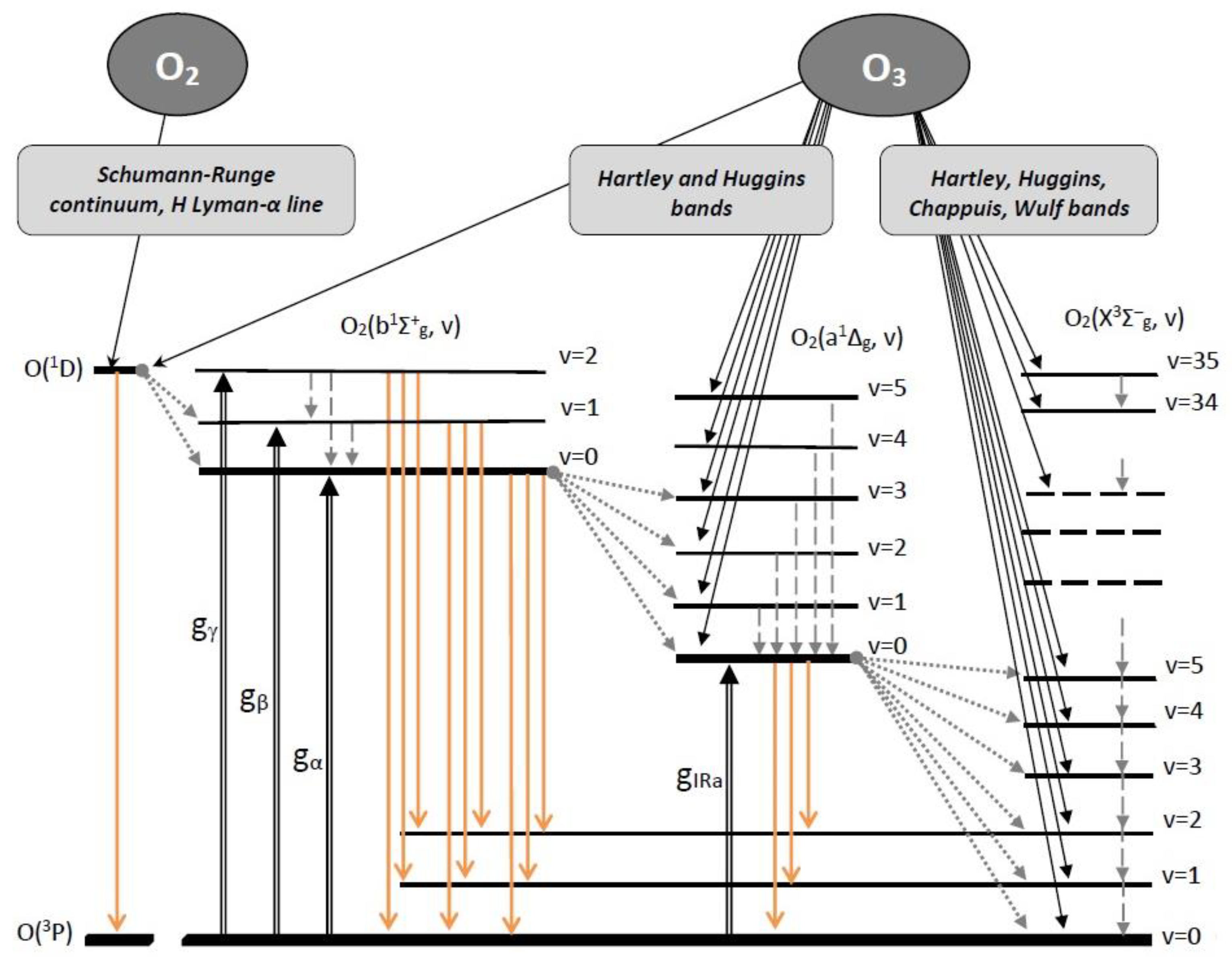
• The most important issue of modern photochemistry is related with a role of O₂(X³Σ_g⁻, v = 1) level [28] which perhaps is a key component in a quasi-resonant energy exchange with H₂O(010) level. Radiance from the H₂O(010) level forms the 6.3 μm band in water vapor. Naturally, energy transfer from the top electronically–vibrationally excited levels of oxygen molecule O₂(a¹Δ_g, v) and O₂(b¹Σ⁺g, v) should be completed by energy transfer between vibrational levels of ground state of oxygen molecule. The aforementioned energy transfer includes several intermediate steps:

  (i)

  O₂(b¹Σ⁺_g, v ≥ 1) → O₂(b¹Σ⁺_g, v = 0);

  (ii)

  O₂(b¹Σ⁺_g, v = 0) → O₂(a¹Δ_g, v ≤ 3);

  (iii)

  O₂(a¹Δ_g, v ≥ 1) → O₂(a¹Δ_g, v = 0);

  (iv)

  O₂(a¹Δ_g, v = 0) → O₂(X³Σ_g⁻, v ≤ 5);

  (v)

  O₂(X³Σ_g⁻, v) + N₂(X¹Σ_g⁺, v′ = 0) → O₂(X³Σ_g⁻, v − 2) + N₂(X¹Σ_g⁺, v′ = 1);

  (vi)

  O₂(X³Σ_g⁻, v > 1) → O₂(X³Σ_g⁻, v = 1);

  (vii)

  O₂(X³Σ_g⁻, v = 1) ↔ H₂O(010).

The reaction (v) is also quasi-resonant and describes two quantum energy transfer from O₂(X³Σ_g⁻, v = 14–25) to N₂(X¹Σ_g⁺, v = 1) (discovered by Park and Slanger [29]). However, energy transfer to O₂(X³Σ_g⁻, v ≥ 1) levels can’t be considered in the framework of MSZ model.

It should be noted that vibrational transitions play an important role in the atmospheric energy transfer. E.g., laboratory experiments from the mid 1970s to the present show that energy transfer as a result of O₂ and O₃ photolysis carried out with participation of electronically–vibrationally excited levels of oxygen molecule. It becomes more clear when considering the mechanism of heating the Earth’s atmosphere due to the absorption of UV radiation from the Sun. Absorbed radiation in the range of 120–900 nm leads to O₂ and O₃ photolysis, and radiation of the Earth’s atmosphere is dominating in the near IR range of spectrum. This spectral range corresponds to radiative vibrational transitions of OH, H₂O, CO₂, CO and other atmospheric species.

The model of electronic–vibrational kinetics of O₂ and O₃ photolysis products in the middle atmosphere which solves all the aforementioned issues and includes the model MSZ as a special case was designed at Atmospheric Physics Department, Saint Petersburg State University [30]. Since 2003, different upgrades of that model have been published [1,2,31,32,33,34,35] etc. The last modified version of the YM2011 will be presented in this study.

The structure of the paper is as follows. Introduction is presented in Section 1. Section 2 describes a procedure of excited oxygen components formation in the daytime MLT. Section 3 presents a detailed description of the YM2011 photochemical model. Possible applications of the YM2011 model are discussed in Section 4. Section 5 includes the conclusions.

2. Formation of Excited Oxygen Components in the Daytime MLT

At first, to model the altitude emission profiles of excited oxygen components, we need to understand the mechanisms of their formation and quenching. In the daytime mesosphere and lower thermosphere (MLT), the main sources of excitation for electronic–vibrational levels of oxygen molecule can be divided into (i) photo processes, namely, absorption of solar radiation by ozone in the Hartley, Huggins, Chappuis, and Wulf bands, and by molecular oxygen in the Schumann–Runge continuum and H Lyman-α line; (ii) processes of resonant absorption of solar radiation. The resonant absorption of solar radiation in bands with centers of 0.762, 0.688, 0.629, and 1.27 μm leads to direct excitation of the O₂(b¹Σ⁺_g, v = 0, 1, 2) and O₂(a¹Δ_g, v = 0), respectively. The rates of these processes are tabulated in [36,37] and traditionally denoted by g_α, g_β, g_γ, and g_IRa.

Basic details of this mechanism became clear in the end of 1970s [4,7,8,38] etc. Photolysis of oxygen molecules leads to formation of excited oxygen atoms O(¹D) due to absorption of solar radiation in the Schumann–Runge continuum, which dominates at altitudes above 90 km, and in the H Lyman-α line whose contribution is in the altitude range of 70–90 km. Below 100 km, another source of O(¹D) formation is ozone photolysis in the Hartley band. As stated earlier [39], at least 90% of solar energy go through formation of excited atom O(¹D) during O₂ and O₃ photolysis. Further, energy of O(¹D) (threshold of excitation of 1.967 eV) is spent on excitation of O₂(b¹Σ⁺_g, v < 2) levels. Figure 1 presents the mechanism of energy transfer between excited oxygen components in the atmosphere.

Note that not only energy transfer from O₂(b¹Σ⁺_g, v < 2) levels is a source of O₂(a¹Δ_g, v ≤ 3) excitation. In the mesosphere, there is one more important source of excitation for O₂(a¹Δ_g, v ≤ 5) levels, namely, singlet channel of ozone photolysis in the Hartley band. Despite many studies still supposing that only O₂(a¹Δ_g, v = 0) level forms in this case, numerous laboratory experiments from 1980 to the present show simultaneous excitation of O₂(a¹Δ_g, v) levels with v up to 5. Only after energy transfer from these levels, does the final population of O₂(a¹Δ_g, v = 0) level occur.

In addition, emission (optical) transitions from each of O₂(a¹Δ_g, v) and O₂(b¹Σ⁺_g, v) levels to the lower O₂(X³Σ_g⁻, v) levels are possible (Figure 1). Traditionally, transitions from these levels are grouped based on the upper excited state. Thus, the transitions O₂(b¹Σ_g⁺, v′ → X³Σ_g⁻, v″) are called the system of atmospheric bands, and the transitions O₂(a¹Δ_g, v′ → X³Σ_g⁻, v″) form the system of IR atmospheric bands. In these systems, transitions (v′ = 0 → v″ = 0) corresponding to the wavelengths of 762 nm and 1270 nm, respectively, are dominant. However, transitions from other vibrational levels are also observed as has been mentioned above. The altitude profiles of volume emission rates (VER) in these transitions let us determine the populations of excited levels of O₂(b¹Σ⁺_g, v) and O₂(a¹Δ_g, v) molecules. That, in turn, allows to track all stages of energy transfer from the upper excited levels to the ground state of oxygen molecules. To model the mechanism shown at Figure 1, we need to know the Einstein coefficients for emission transitions and have a database of rate coefficients for reactions of energy transfer and quenching of excited oxygen components in collisions with the main atmospheric components, namely, O₂, N₂, O₃, O(³P), CO₂. The role of the other small atmospheric components is neglectable in collisional processes [35].

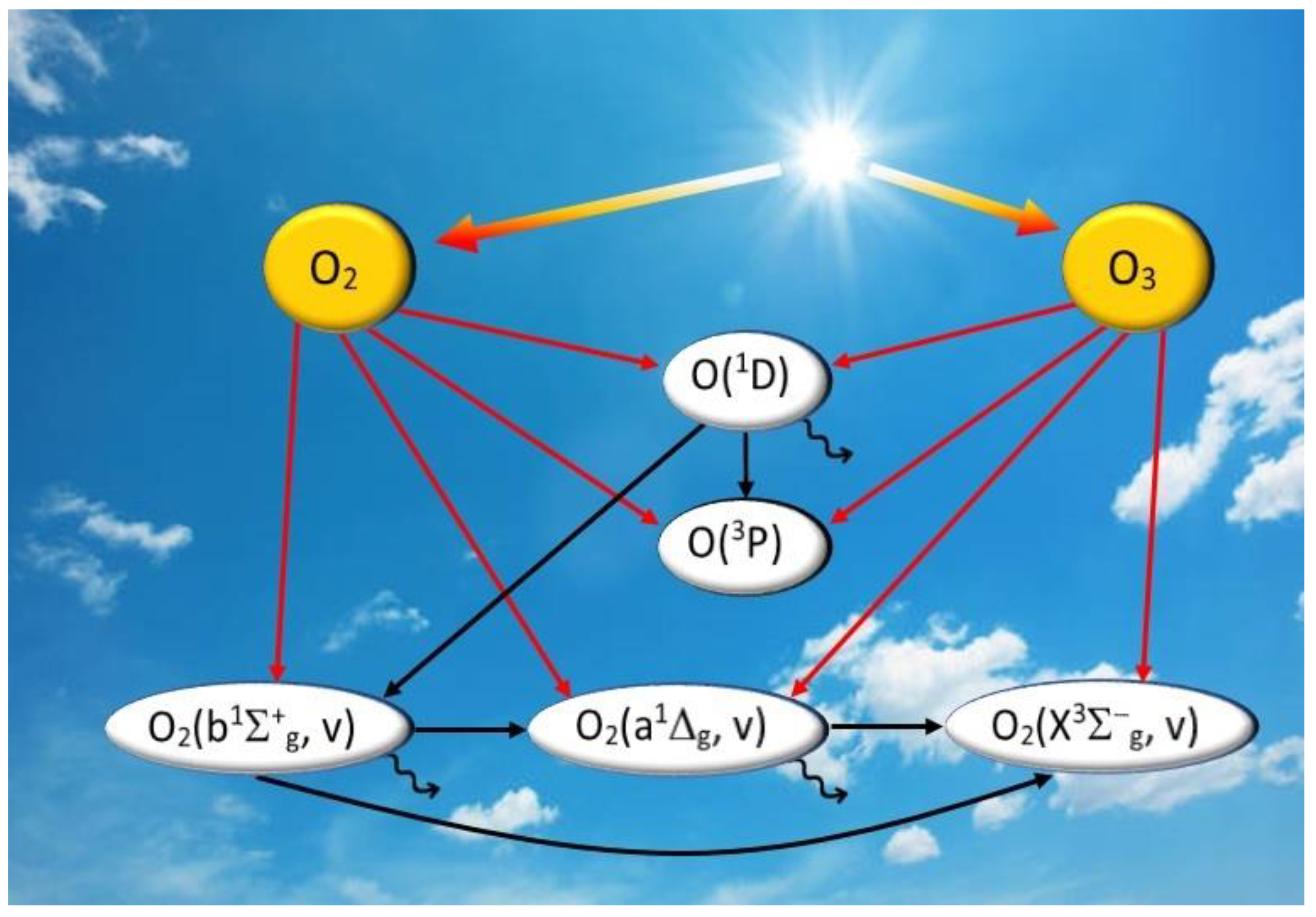
2.1. O₃ Photodissociation and Its Products

As has been mentioned, there are two channels of O₃ photodissociation:

(i)

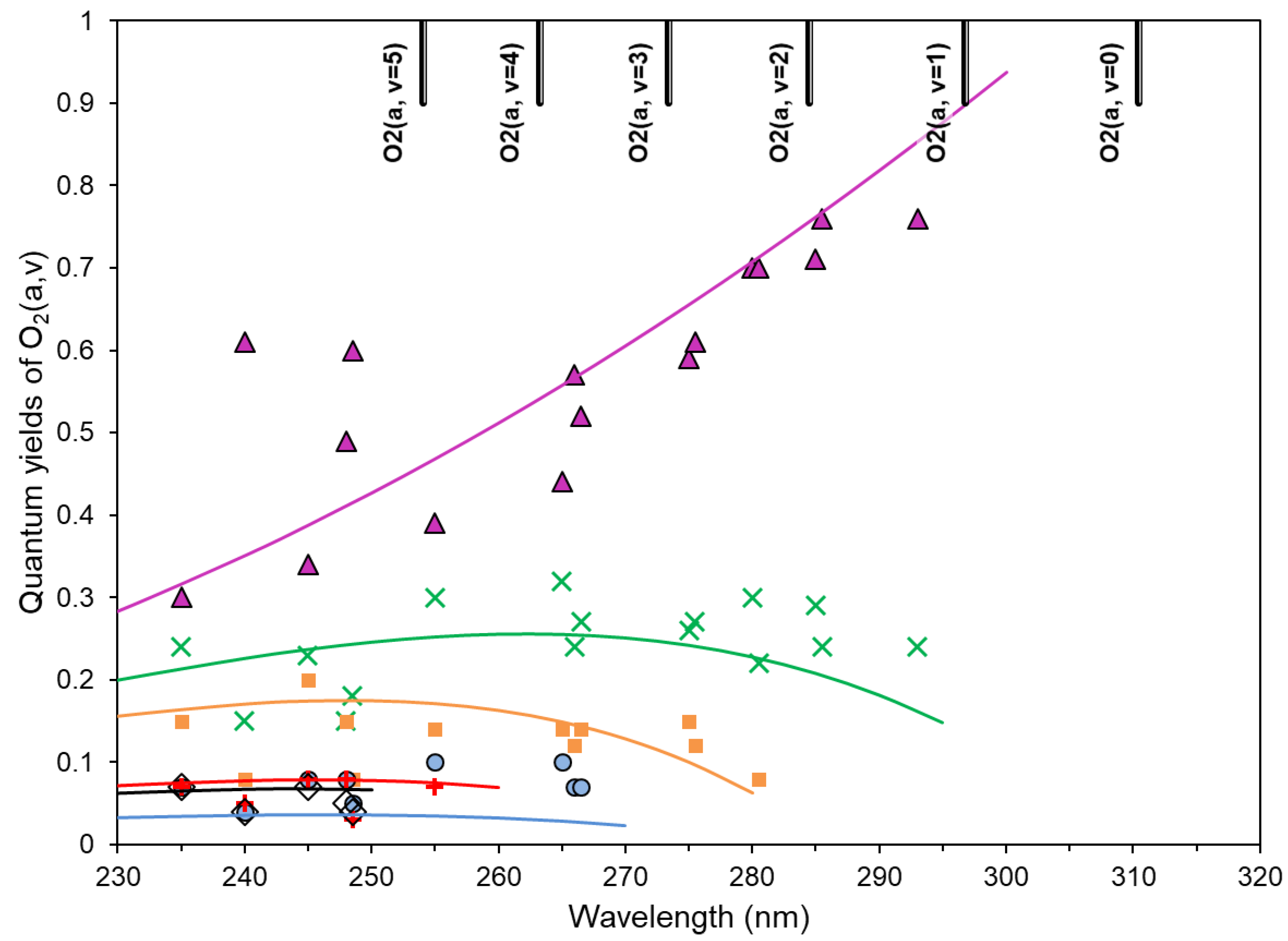
singlet channel O₃ + hv (λ = 200–320 nm) → O₂(a¹Δ_g, v = 0–5) + O(¹D) in Hartley band;

(ii)

triplet channel O₃ + hv (λ = 200–900 nm) → O₂(X³Σ⁻_g, v = 0–35) + O(³P) in Hartley, Huggins, Chappuis and Wulf bands.

In this subsection we will focus on the singlet channel since the dependence of O₂(X³Σ⁻_g, v ≤ 35) quantum yields in triplet channel on wavelength has already been studied by Svanberg et al. [40] (Figure 2). Experimental studies of quantum yield in singlet channel for fixed wavelengths have also been performed [41,42,43,44], however, statistical processing of the results was not carried out. Note, that discrete data are not convenient for analytical studies, as these data require further interpolation. Therefore, here we will shortly consider analytical description of O₂(a¹Δ_g, v) quantum yields in singlet channel of ozone photolysis depending on wavelength. More detailed description of this analytical approach can be found in [45,46,47].

The feature of photodissociation is changing of photolysis products and quantum yields depending on wavelength. Thus, there are threshold wavelengths starting from which oxygen molecules O₂(X³Σ⁻_g, v) and O₂(a¹Δ_g, v) with higher vibrational level v are formed (

Table 1. Threshold wavelengths λ used to calculate threshold value of x and normalization factors C_v.

Products of O3 Photodissociation in Hartley Band	O2(a1Δg, v)
	v = 0	v = 1	v = 2	v = 3	v = 4	v = 5
Threshold wavelength, nm	310	296	284	273	263	254
Threshold value of x	0.937	0.689	0.576	0.483	0.407	0.339
Cv	1.068	1.233	0.564	0.375	0.377	0.473

).

The energy mismatch of the reaction (i) can be written as:

ΔE = E − E_DissO3 − E_O(1D) − E_{O2(a, v=0)},

(1)

where E is the energy of photon, E_DissO3 is the energy of ozone dissociation (1.05 eV), E_O(1D) is the energy of O(¹D) excitation with respect to the ground state (1.967 eV), and E_{O2(a, v=0)} is the energy of O₂(a¹Δ_g, v = 0) excitation with respect to the ground state (0.977 eV).

Next, we introduce the parameter x determining the fraction of O₂(a¹Δ_g, v) molecules which have energy above the excitation threshold of the O₂(a¹Δ_g, v = 0) level:

$$x=\exp \left(-\frac{\Delta E}{E_{O2\left(a,v=0\right)}}\right)$$

(2)

Then, the quantum yield of O₂(a¹Δ_g, v) is determined by the fraction of energy that goes to the excitation of this level, depending on the wavelength and can be calculated by formulas:

F_a,0 (x) = C₀ x for v = 0

(3)

$$F_{a,v}\left(x\right)=C_{v}x\left(1-x-\frac{x^2}{2}-\frac{x^3}{2^2}-\cdots -\frac{x^v}{2^{v-1}}\right)\mathrm{for}\mathrm{v}\ge 1$$

(4)

where C_v are normalization factors which have been calculated based on condition that the sum of quantum yields of all vibrationally excited O₂(a¹Δ_g, v) molecules equals 1 (Table 1). Each normalization factor was calculated at a threshold energy value starting from which an oxygen molecule with the next vibrational level is formed during photolysis (x in Table 1 and the upper scale of Figure 3). Figure 3 represents the comparison of all currently known experimental values of F_a,v (symbols) with calculations by Equations (3) and (4) (solid lines). It is clearly seen from Figure 3 that molecules O₂(a¹Δ_g, v = 0–5) are formed simultaneously at the peak of the Hartley band cross section absorption (wavelength of ∼254 nm). Moreover, the quantum yield of O₂(a¹Δ_g, v = 0) formation does not exceed 45%.

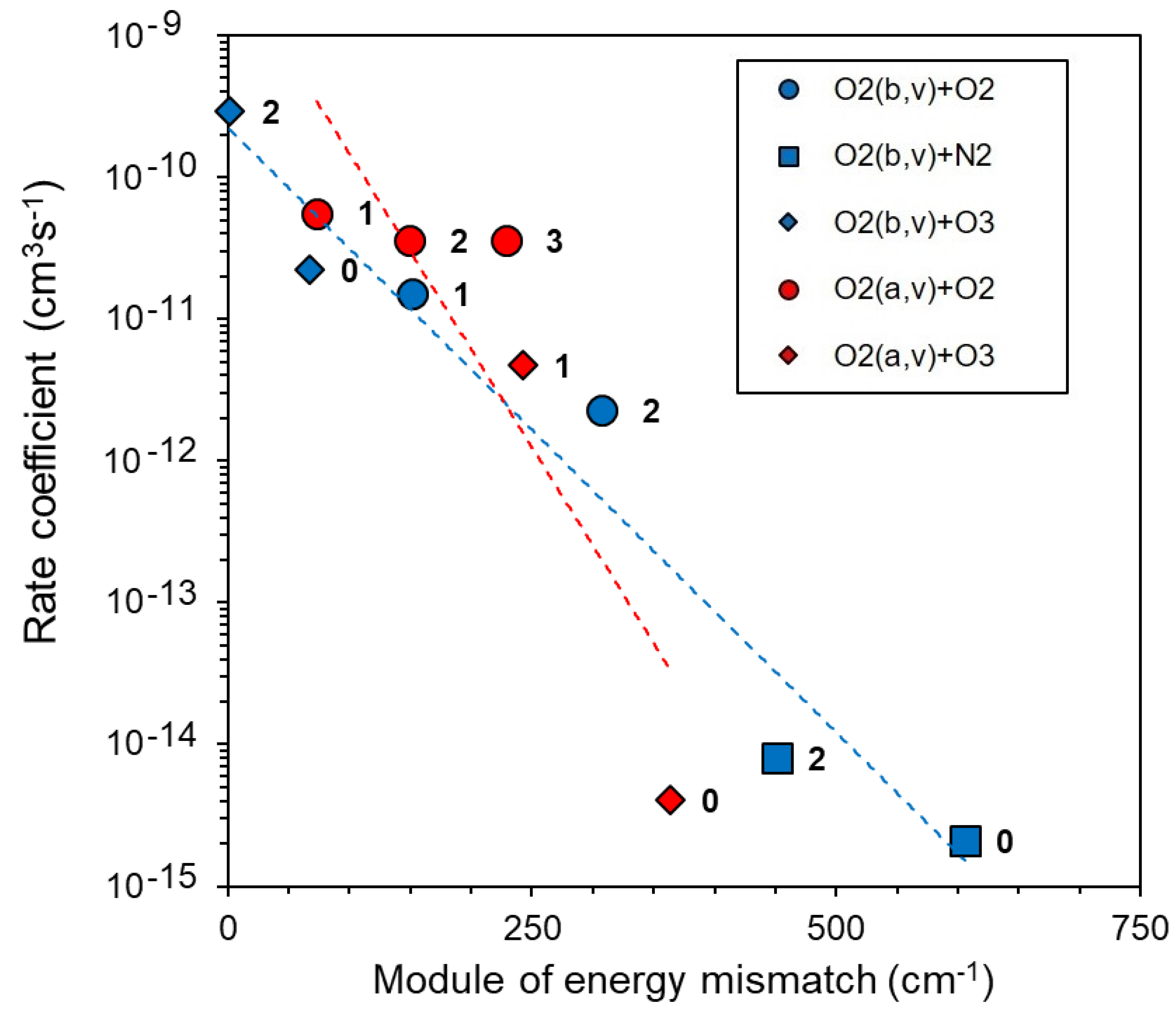
2.2. Energy Transfer in Collisional Reactions

Summarizing the discussion above the following may be stated. (1) An excited O(¹D) atom and oxygen molecules in the states O₂(a¹Δ_g, v = 0–5) and O₂(b¹Σ_g⁺, v = 0–2) are formed as a result of photolysis. (2) Further, the energy of these excited levels is transferred to the lower excited levels of the oxygen molecule as a result of radiation and collision processes (see Figure 1). Note, however, that reaction rate coefficients involving electronically–vibrationally excited molecules are difficult for experimental measurements by traditional methods.

Progress in building a new model of electronic–vibrational kinetics of oxygen components began in the late 90 s-early 2000 s. At first, the coefficient of vibrational-vibrational relaxation of the oxygen molecule ground electronic state O₂(X³Σ⁻_g, v) in the reaction

O₂(X³Σ⁻_g, v′ ≤ 13) + O₂ → O₂(X³Σ⁻_g, v′ − 1) + O₂(X³Σ⁻_g, v = 1)

(5)

was measured by Klatt et al. [48] and was calculated by Hernandez et al. [49]. It has been shown that the rate coefficient of reaction (5) decreases with an increase of the vibrational number.

In 1994, another interesting result was obtained by Park and Slanger [29], namely, a sharp resonant increase of the reaction (6) rate for v′ = 14–25 due to the transfer of energy of two vibrational quanta of an oxygen molecule to one vibrational quantum of a nitrogen molecule.

O₂(X³Σ⁻_g, v′ = 14–25) + N₂ → O₂(X³Σ⁻_g, v′ − 2) + N₂(X¹Σ_g⁺, v = 1)

(6)

The fact is that for such v′ values in reaction (6), the energy transfer from the oxygen molecule to the nitrogen molecule has an almost resonant character. In both (5) and (6) cases, it is obvious that a change in the reaction rate coefficient with a change in v is associated with a defect of the reaction energy (see Figure 4 where both experimental data [29,48,50,51,52,53,54] and theoretical estimates [55] are presented). The smaller defect of energy, the greater the reaction rate coefficient. Figure 4 shows rate coefficients of the reactions (5)–(6) depending on module of energy mismatch.

Since 1998, a series of experiments was begun at the Molecular Physics Laboratory (MPL), SRI International (Space Research Institute) to measure rate coefficients of reactions involving electronically vibrationally excited oxygen molecules in the two singlet states, O₂(b¹Σ_g⁺, v ≥ 1) and O₂(a¹Δ_g, v ≥ 1), in collisions with atomic and molecular oxygen, as well as with nitrogen. As a result of the experiments, it was found that the rate coefficients of these reactions have abnormally high values close to the gas–kinetic reaction rates [56,57,58,59] etc. In a certain sense, this was a kind of surprise, since the reaction rate coefficients for singlet levels of oxygen molecule without vibrational excitation were low. For example, reaction rate coefficients for

O₂(a¹Δ_g, v = 0) + O₂ → products

(7)

O₂(b¹Σ_g⁺, v = 0) + O₂ → products

(8)

have values of k(O₂(a, v = 0); O₂) = 3 × 10⁻¹⁸ cm³ s⁻¹ and k(O₂(b, v = 0); O₂) = 4 × 10⁻¹⁷ cm³ s⁻¹ [60]. The MPL laboratory staff were able to explain the sharp acceleration of the reactions for v ≥ 1 by the fact that these reactions proceed through the channel of electron–vibrational exchange, namely,

O₂(a¹Δ_g, v′) + O₂(X³Σ⁻_g, v″ = 0) → O₂(X³Σ⁻_g, v′) + O₂(a¹Δ_g, v″ = 0)

(9)

O₂(b¹Σ_g⁺, v′) + O₂(X³Σ⁻_g, v″ = 0) → O₂(X³Σ⁻_g, v′) + O₂(b¹Σ_g⁺, v″ = 0)

(10)

A feature of these reactions is that the quantum of electronic excitation is transmitted to the partner through a collision, and the quantum of vibrational excitation is “frozen” as it is. These reactions have an energy defect in the range of 0–250 cm⁻¹. Typical rate coefficients of these reactions for v = 1, 2, 3 have values of (0.5–5.0) × 10⁻¹¹ cm³ s⁻¹, that is, they are only several times lower than the gas-kinetic rate of the chemical reaction (see Figure 5). Another feature of these reactions is that, with an increase of vibrational excitation, the rate coefficients of these reactions usually begin to decline (see Figure 5).

It would be natural to expect that a similar effect should be observed in collisional reactions with ozone. Indeed, the rate coefficients measured at room temperature are k(O₂(a, v = 0); O₃) = 4 × 10⁻¹⁵ cm³ s⁻¹ for O₂(a¹Δ_g, v = 0) and k(O₂(a, v = 1); O₃) = 5 × 10⁻¹² cm³ s⁻¹ for O₂(a¹Δ_g, v = 1). A similar dependence of the reaction rate coefficient on the energy defect is also observed for collisional reactions of O₂(b¹Σ_g⁺, v = 0) with ozone (Figure 5):

O₂(b¹Σ_g⁺, v = 0) + O₃ → O₂(a¹Δ_g, v = 0) + O₃(302) + 67.6 cm⁻¹

(11)

O₂(b¹Σ_g⁺, v = 2) + O₃ → O₂(a¹Δ_g, v = 2) + O₃(203) + 2.0 cm⁻¹

(12)

Of particular interest are the collisional reactions of electronically–vibrationally excited oxygen molecules with atomic oxygen. To date, the products of these reactions are not known, however, their rate coefficients have a rather large scatter of values (see

Table 2. Possible correlation between a reaction energy mismatch and value of the rate coefficient at thermal temperatures.

No.	Reaction	Rate Coefficient, cm3 s−1 [2]	Supposed Products of Reaction	Energy Mismatch, cm−1
1	O2(b1Σg+, v = 2) + O(3P) →	1.07 × 10−11	O2 + O(1D)	37.6
2	O2(b1Σg+, v = 1) + O(3P) →	4.5 × 10−12	O2(X3Σg−, v = 10) + O(3P)	2.3
3	O2(b1Σg+, v = 0) + O(3P) →	8 × 10−14	O2(a1Δg, v = 0) + O(3P)	5238.0
4	O2(a1Δg, v = 0) + O(3P) →	<3 × 10−16	O2 + O(3P)	7883.0

). Such a spread of values can be explained if we assume that only a part of these reactions (the fastest) are quasi-resonant. For example, in Table 2 we offer possible products of a number of reactions and energy defects corresponding to these channels. So, the first very fast reaction is apparently quasi-resonant, as a result of which the energy of the O₂(b¹Σ_g⁺, v = 2) molecule, as we believe, is transferred to the O(¹D) atom. The energy defect of this reaction in this channel is only 37.6 cm⁻¹ (or 54 K). In passing, we note that at higher kinetic temperatures of the gas, a quasi-resonant process in the reverse reaction may be possible

O(¹D) + O₂ → O(³P) + O₂(b¹Σ_g⁺, v = 2) − 37.6 cm⁻¹

(13)

The results of a laboratory experiment suggest this idea [61].

A high value of the rate coefficient for the second reaction in Table 2 can be, presumably, due to the fact that the energy transfer goes to the excitation of oxygen molecules with the vibrational level v = 10. However, this assumption requires experimental confirmation. For the last two reactions in Table 2 with low values of the rate coefficients, it was not possible to find quasi-resonant energy transfer channels.

It must be emphasized that at present, the rate coefficients of reactions involving atomic oxygen are measured with a very large error. For example, the rate coefficient of reaction 4 in Table 2 is known only as the upper limit, k(O₂(a, v = 0); O(³P)) < 3 × 10⁻¹⁶ cm³ s⁻¹ [1], and the rate coefficient k(O₂(b, v = 0); O(³P)) has a large relative error ∼400% [60].

To date, for only one reaction involving atomic oxygen, theoretical calculations of the reaction rate coefficient depending on the values of the vibrational quantum have been carried out, namely, for

O₂(X³Σ⁻_g, v ≤ 30) + O(³P) → O₂(X³Σ⁻_g, v′ = v − Δv) + O(³P)

(14)

Esposito et al. [62] calculated the values of the reaction (14) rate coefficients for Δv = 1–30 (see Figure 6). This reaction turned out to be one of the keys for modeling population of O₂(X³Σ⁻_g, v′ = 1) level in the MLT region [33,34]. A distinctive feature of this mechanism is that in order to populate the lower vibrational level O₂(X³Σ⁻_g, v′ = 1), cascade transitions from all overlying levels v′ = 2–30 must be considered.

Using experimental studies [5,48,58,61,63,64,65,66,67] etc. as well as theoretical calculations by [62,68,69,70] we managed to create a database of the rate coefficients and quantum yields of reaction products with the participation of O₂(b¹Σ_g⁺, v), O₂(a¹Δ_g, v), O₂(X³Σ⁻_g, v) [33], (supplement in 2). This database was the basis of the model of electronic–vibrational kinetics of O₂ and O₃ photolysis products in the MLT region (YM2011 model). It is important to emphasize that for a significant part of reactions in the database, temperature dependence and the error range for the MLT temperature range are known.

2.3. Emission Transitions

Emission transitions O₂(b¹Σ⁺_g, v′ ≤ 10 → X³Σ⁻_g, v″), O₂(a¹Δ_g, v′ ≤ 10 → X³Σ⁻_g, v″) and O₂(b¹Σ⁺_g, v′ ≤ 10 → a¹Δ_g, v″) form the systems of O₂ atmospheric, IR atmospheric, and Noxon bands, respectively. The population of an excited level is related with volume emission rate (VER) from this level to the lower level as the ratio of VER to the Einstein coefficient for the corresponding transition, A_E. Therefore, Einstein coefficients are necessary to calculate concentrations of the excited molecules O₂(b¹Σ⁺_g, v′ ≥ 0) and O₂(a¹Δ_g, v′ ≥ 0) in the MLT from measured VERs. In addition, Einstein coefficients are related to the radiative quenching which is the key process in the lower thermosphere.

Currently, there is no single database of Einstein coefficients for the aforementioned transitions in O₂ bands, however, some attempts to define them from both measurements and theory have been made.

Table 3. Measured values of Einstein coefficient (s⁻¹) for O₂ bands systems [72,73].

Transition.	v′ = 0		v′ = 1		v′ = 2		v′ = 3
	v″ = 0	v″ = 1	v″ = 0	v″ = 1	v″ = 0	v″ = 1	v″ = 0	v″ = 1
O2 Atm band (v′-v″)	8.93 × 10−2	4.67 × 10−3	7.20 × 10−3	7.01 × 10−2	2.69 × 10−4		6.73 × 10−6
O2 Noxon band (v′-v″)	1.20 × 10−3
O2 IR Atm band (v′-v″)	2.26 × 10−4	2.81 × 10−6

shows all values of the Einstein coefficients obtained in laboratory studies.

Table 4. Calculations of Franck–Condon factor values.

Details of Calculation.	Transitions	Reference
Morse potential	O2(b, v′ ≤ 3 ↔ X, v″ ≤ 3)	[72]
	O2(b, v′ ≤ 3 ↔ a, v″ ≤ 5)
	O2(a, v′ ≤ 5 ↔ X, v″ ≤ 6)
RKR potential	O2(b, v′ ≤ 3 ↔ X, v″ ≤ 8)	[73]
	O2(a, v′ ≤ 3 ↔ X, v″ ≤ 6)
RKR potential	O2(b, v′ ≤ 4 ↔ X, v″ ≤ 4)	[23]
Transition moments from [74]	O2(b, v′ ≤ 10 ↔ X, v″ ≤ 9)	[25]
RKR potential	O2(b, v′ ≤ 10 ↔ X, v″ ≤ 35)	[71]
	O2(b, v′ ≤ 10 ↔ a, v″ ≤ 15)
	O2(a, v′ ≤ 10 ↔ X, v″ ≤ 35)

includes information about attempts to calculate the Einstein coefficients for last 50 years. The data incompleteness does not allow to sufficiently describe the radiative quenching in photochemical modelling. Therefore, Yankovsky et al. [2] presented an estimation of the Einstein coefficients for emission transitions in the O₂ atmospheric, IR atmospheric, and Noxon bands based on values of the Franck–Condon factor from [71].

The spectroscopic parameters of mentioned transitions were specified in laboratory experiments and theoretical calculations [72,73,74,75,76,77,78,79,80,81] etc. A part of the results is used in the last version of HITRAN (only for transitions from levels v ≤ 2).

Yankovsky et al. [2] calculated the Einstein coefficients $A_{v^{\prime }{v}^{″}}$ using the formula from [82,83]:

$$A_{{\mathrm{v}}^{\prime }{\mathrm{v}}^{″}}=A_{00}\frac{q_{{\mathrm{v}}^{\prime }{\mathrm{v}}^{″}}{\nu }_{{\mathrm{v}}^{\prime }{\mathrm{v}}^{″}}^3}{q_{00}{\nu }_{00}^3}$$

(15)

where $v_{v^{\prime }{v}^{″}}$–transition energy in cm⁻¹, $q_{v^{\prime }{v}^{″}}$–Franck-Condon factor for transition from the level with vibrational number v′ to the level with vibrational number v″, taken from [71]. Results of calculations by (15) for the atmospheric, Noxon, and IR atmospheric bands, respectively, are presented in [2].

The values of the Einstein coefficient for transitions from v′ = 0–10 to v″= 0–14 in the O₂ atmospheric band [2] allow us to estimate the probability of radiative quenching for levels O₂(b¹Σ_g⁺, v′ = 0–10) (Figure 7). Notice that our estimation of the radiative lifetime based on the Einstein coefficients from [2] is consistent with recent experimental estimates for vibrational levels v = 0, 1. Differing from our calculation, the data from [84,85] were estimated only on the basis of values for the fundamental transitions O₂(b¹Σ_g⁺, v′ = 0, 1 → X³Σ⁻_g, v″ = 0, 1) and do not take into account emission transitions to levels v″ > 1.

2.4. Another Mechanism of O₂(b¹Σ⁺_g, v = 0) Excitation

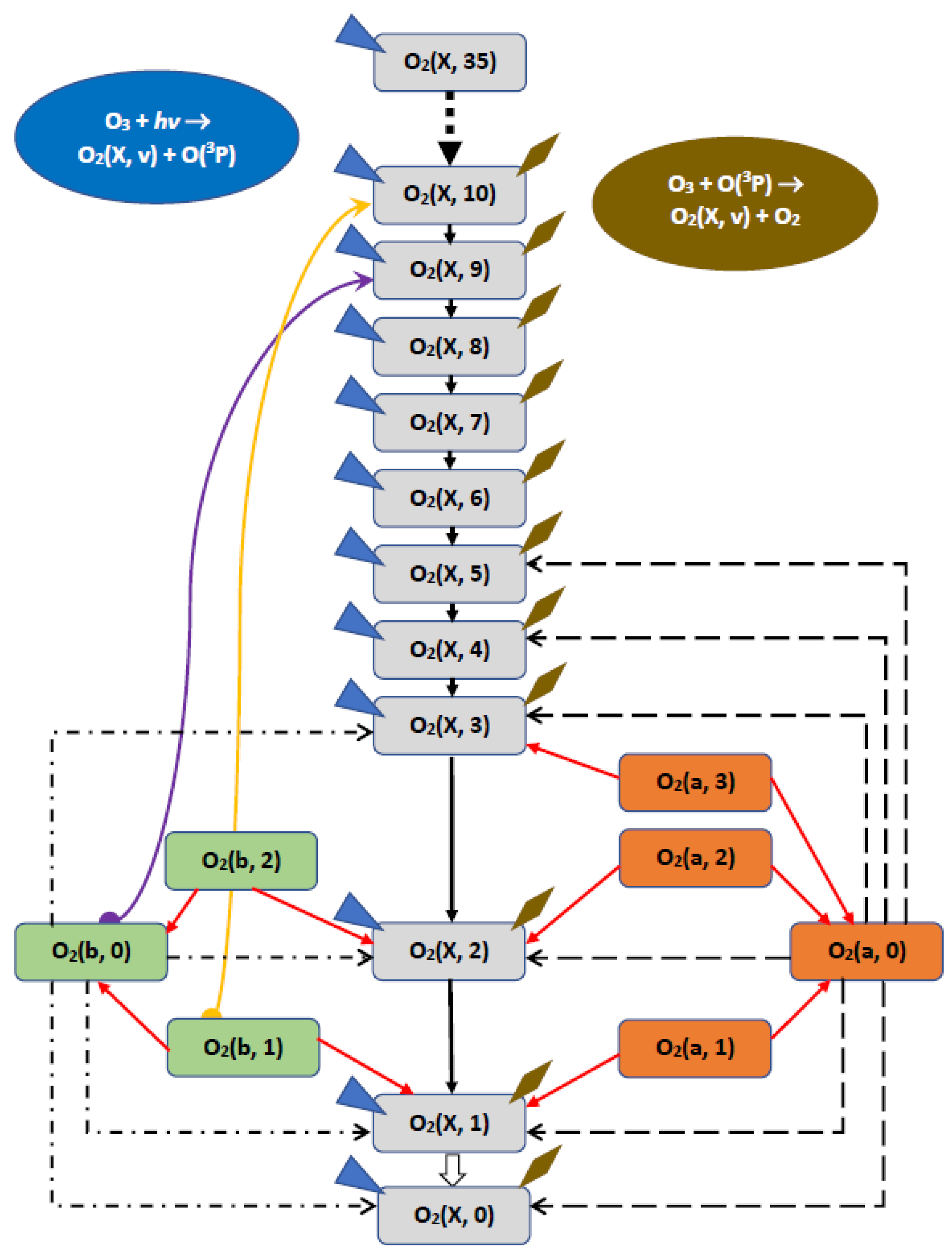
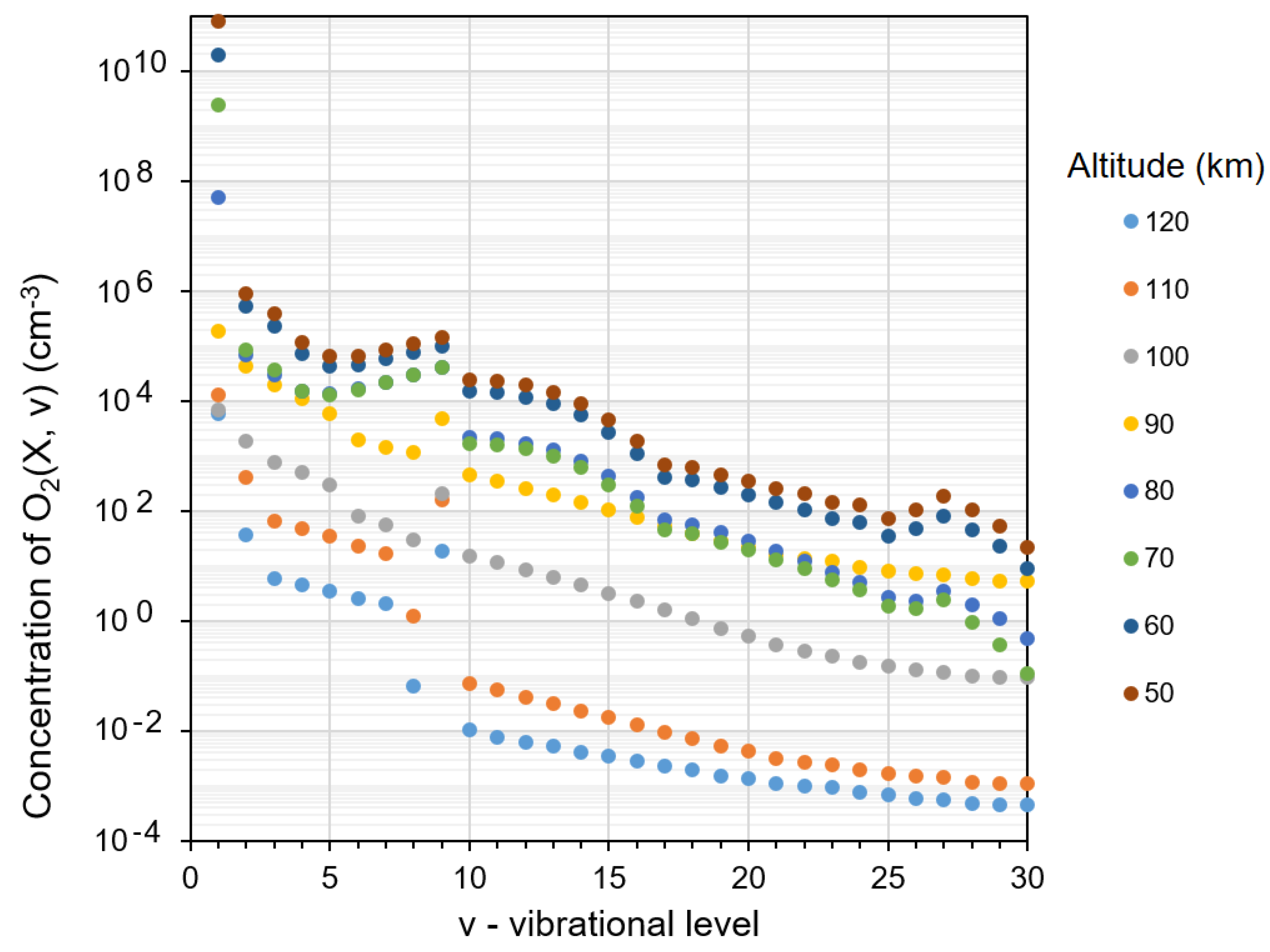
It should be noted that there is another source of energy in lower thermosphere - the association of oxygen atoms in the triple reaction

O(³P) + O(³P) + M → O₂(precursor) + M + 5.12 eV

(16)

As was shown in the early 1970s, this exothermic reaction is a source of excitation of the O(¹S) atom in the nightglow (for example, in [88]) within the framework of the Barth’s mechanism:

O₂(precursor) + O(³P) → O₂ + O(¹S)

(17)

However, under the same Barth’s mechanism, energy can be transferred to excite singlet or triplet levels of the oxygen molecule, in two ways. Either a one-step channel in reaction (16), or a two-step channel, sequentially (16) and the subsequent energy transfer in the reaction:

O₂(precursor) + O₂ → O₂ + O₂(electronic state)

(18)

All these proposed energy transfer channels were tested in the course of the beautifully conceived multi-rocket experiment ETON in March 1982. For each of the considered energy transfer channels, corresponding parameterizations were obtained, which have been used up to now [15,16,17] etc.

In recent years, using data from new rocket experiments, upgraded parameterizations have been proposed for the formation of O₂(b¹Σ_g⁺, v = 0) molecules [18,19]. Figure 8 shows the contribution of the Barth’s mechanism to the formation of the altitude profile of O₂(b¹Σ_g⁺, v = 0) concentration in dayglow based on several SABER events and three parameterizations [15,18,19]. Unfortunately, the uncertainties of these parameterizations remain too large. But the uncertainty of the atomic oxygen altitude profile above 80 km can introduce a much larger error, since the efficiency of the Barth’s mechanism is proportional to the square of O(³P) concentration according to formula (16). Therefore, the selection of test events was motivated by significantly different altitude profiles of atomic oxygen (left panel in Figure 8). While at nightglow this mechanism dominates in the altitude range of 90–103 km, during the daytime its contribution compared to photolysis of O₂ and O₃ varies from fractions of a percent to a few percent according to estimations by [24,89] etc. (compare with our estimations in Figure 8, right panel). Thus, for daytime conditions, the assessment of the Barth’s mechanism contribution to the population of the singlet level of the oxygen molecule is so far only qualitative.

2.5. Kinetics of O₂(X³Σ⁻_g, v) in MLT

As mentioned above, in order to calculate the population of the O₂(X³Σ⁻_g, v = 1) level, it is necessary to take into account the processes of energy transfer to this level from all overlying excited levels of the oxygen molecule, namely O₂(b¹Σ_g⁺, v = 0–2), O₂(a¹Δ_g, v = 0–5), O₂(X³Σ⁻_g, v = 2–35). To calculate the concentration of O₂(X³Σ⁻_g, v = 1), we solved a system of 45 kinetic equations for O(¹D) and the above-mentioned excited components. A block scheme of this mechanism (Figure 9) was developed by [33,34]. In these papers and in [1,2] latest version of database, one can find a database of reaction rate coefficients for the formation and quenching of molecules O₂(X³Σ⁻_g, v = 1–35) with corresponding links. We note that in the two most common databases on chemical kinetics and photochemical data, namely, [90] and [60], there are no data on reaction rate coefficients involving electronically–vibrationally excited atmospheric components.

Key feature of the model shown in Figure 9 is that to populate the lowest level of O₂(X³Σ¯_g, v = 1), it is necessary to consider the five main channels of vibrational excitation for the three lower electronic levels of the oxygen molecule:

(1)

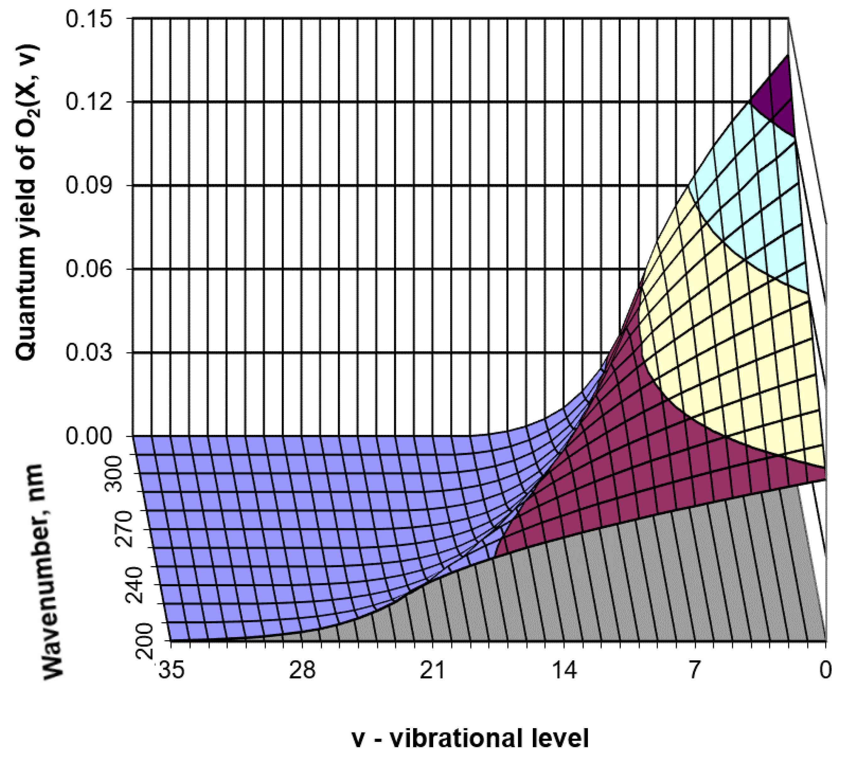
Direct population of O₂(X³Σ¯_g, v = 1–35) as a result of ozone photolysis (in the triplet channel) in the Hartley, Huggins, Chappuis, and Wulf bands. Moreover, the photodissociation rate substantially depends on the wavelength of solar radiation, as can be seen from Figure 2. The methodology for calculating rates of the photodissociation processes which sequentially takes into account threshold values of the excitation for each vibrational level is described in detail in [33,46].

(2)

Direct simultaneous population of O₂(X³Σ¯_g, v = 1−30) in the reaction O₃ + O(³P) → O₂(X³Σ^¯_g, v = 0–30) + O₂ whose rate coefficient is highly dependent on kinetic temperature [60,91].

(3)

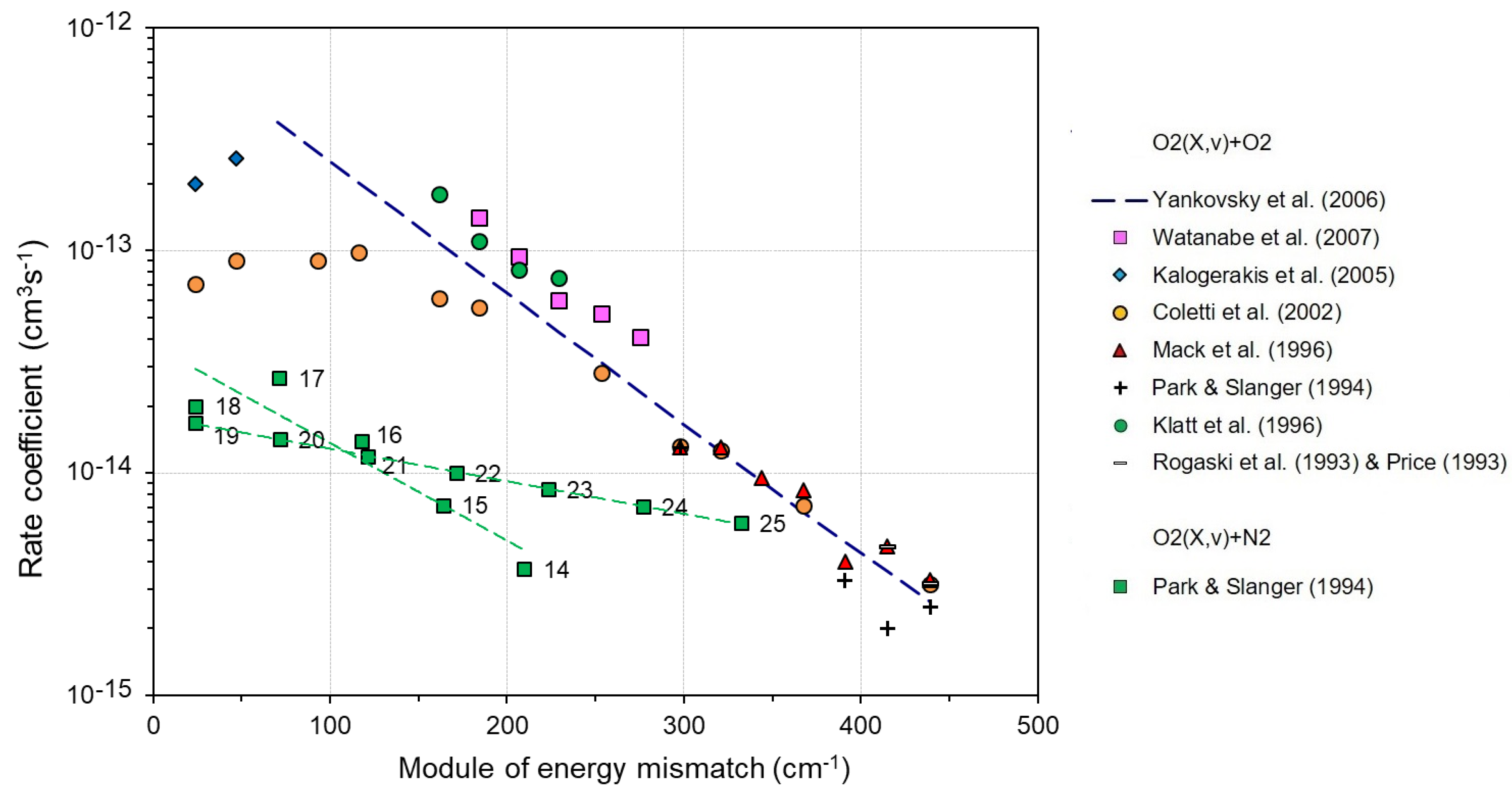
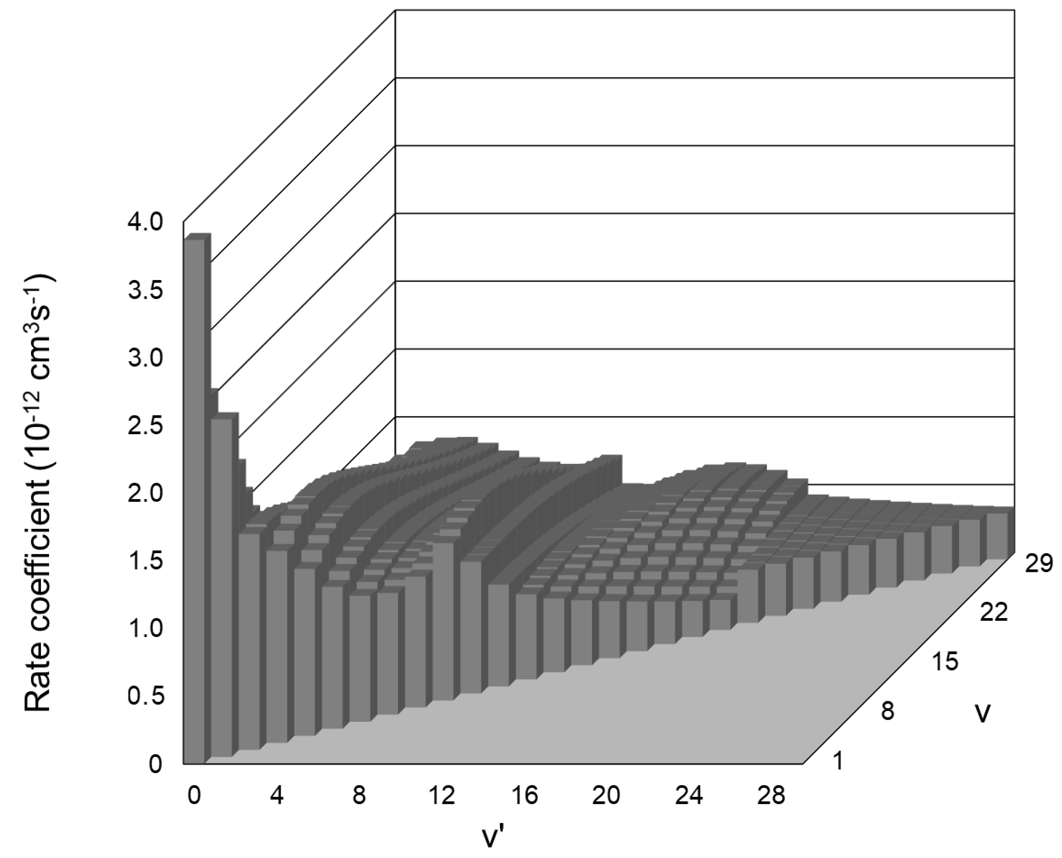
Cascade population of each O₂(X³Σ¯_g, v) level due to transitions from all overlying (with respect to it) levels as a result of reaction (14). The rate coefficients of all cascade transitions were calculated by [62] and visualized by us in Figure 6. The term which takes into account the contribution of mentioned cascade transitions in the kinetic equation for O₂(X³Σ⁻_g, v) is

$$\mathrm{Production}\left(O_2\left(X^3{\Sigma }_g^{-},v\right)\right)=[O{(}^{3}P)]\cdot {\displaystyle \sum }_{m=v+1}^{30}[O_2\left(X^3{\Sigma }_g^{-},m\right)]\cdot k\left(O_2\left(X,m\right);O{(}^{3}P\right))$$

(19)

Thus, we have to consider 464 cascade transitions to describe the population of the O₂(X³Σ⁻_g, v = 1) level only.

(4)

Energy transfer from O₂(b¹Σ⁺_g, v ≤ 2) and O₂(a¹Δ_g, v ≤ 5) levels as a result of fast reactions (9), (10).

(5)

The processes of (V–V) and (V–T) vibrational relaxation in collisions with O₂ and N₂ (see Section 2.2).

The channels (2–5) continue to be the most effective in the O₂(X³Σ⁻_g, v = 1–30) kinetics in nighttime mesosphere, however, this problem has not yet been solved by anyone.

The algorithm proposed in Figure 9 allows one to calculate the daytime distribution of O₂(X³Σ⁻_g, v = 1–35) molecules in the altitude range of 50–120 km (an example of calculation for v = 1–35 is shown in Figure 10) depending on the date, latitude, and zenith angle of the sun.

Figure 11 gives an example of calculating the altitude profiles of the concentrations of O₂(X³Σ⁻_g, v = 1) and O₂(X³Σ⁻_g, v = 2) for different solar zenith angle (SZA) during one day (based on the TIMED-SABER data [92] on the atmospheric composition and SORCE data [93] on the spectral characteristics of solar radiation in the range 120–900 nm). A characteristic feature of these altitude profiles is the low variability of these profiles during daylight hours, at least for SZA ≤ 85. In addition, it is necessary to pay attention to the abnormally high concentration of O₂(X³Σ⁻_g, v = 2) molecules in the altitude range 90–100 km (the threshold of excitation of this level of the oxygen molecule is 3089 cm⁻¹).

To simulate the altitude profile of O₂(X³Σ⁻_g, v = 1) concentration in various geophysical situations, we used a set of standard atmospheric models TROP (TROPics), SAS (SubArctic Summer), MLW (Middle-Latitude Winter), MLS (Middle-Latitude Summer), as well as fifty SABER events for summer equinox. We presented all these profiles as functions of atmospheric pressure (Figure 4, from [34]). It was possible to obtain a universal altitude profile of the resulting quantum output (RQO) of the production of O₂(X³Σ⁻_g, v = 1) molecules per act of ozone photolysis in the Hartley, Huggins, Chappuis, and Wulf bands for the altitude range of 50–90 km depending on atmospheric pressure. It turned out that the shape of the altitude distribution of RQO weakly depends on the date, latitude and SZA [34].

3. Kinetics of O₂ and O₃ Photolysis Products in MLT. The Modern Model

All processes considered in Section 2 were taken into account in the kinetics model of O₂ and O₃ products. The first publication of the model was in 2003 [30], the first full-functional version of the model was published in 2006 [32], the upgrade version YM2011 (Figure 12) was presented in publications 2011–2019. In the framework of the YM2011 model, the concentrations of the molecules O₂(X³Σ_g⁻, v = 1–35), O₂(a¹Δ_g, v = 0–5), O₂(b¹Σ_g⁺, v = 0–2) are calculated from the solution of the system of kinetic equations for these excited levels. The system of kinetic equations can be solved analytically, considering the hierarchical location of the excited levels as a function of energy.

In the formation of altitude distributions of the vibrational level populations of the oxygen molecule in the ground electronic state O₂(X³Σ_g⁻, v = 1–35) we took into account not only the direct excitation channel, namely, ozone photolysis in the Hartley, Huggins, Chappuis, and Wulf (200‒900 nm) bands, but also transfer of energy from excited levels of O₂(a¹Δ_g, v = 0–5) and O₂(b¹Σ_g⁺, v = 0, 1, 2) which are populated both as a result of ozone photolysis in the Hartley band, and as due to energy transfer from the excited oxygen atom O(¹D).

In the new version of the YM2011 model (Figure 12), we first took into account the additional channels for the formation of O(¹D) atoms during the photolysis of ozone in the Huggins band, as well as the energy transfer from O₂(b¹Σ⁺_g, v = 0, 1) to O₂(X³Σ⁻_g, v = 9 and 10).

The YM2011 model is self-consistent and allows you to solve both forward and inverse problems. By the forward problem, we mean the calculation of altitude profiles of concentration of excited oxygen components in the MLT region. Bear in mind that the concentration of molecules in the excited state is related with volume emission rate (VER) through the Einstein coefficient (Section 2.3). Thus, in the framework of the YM2011 model, for different atmospheric conditions (season, latitude, zenith angle of the sun, etc.) the altitude distributions of volume emission rates can be calculated not only for traditional oxygen bands of O₂ IR Atm (0, 0) at 1.27 μm and O₂ Atm (0, 0) at 0.762 μm, but also for the systems of O₂ atmospheric, IR atmospheric, and Noxon bands (Section 2.3). The calculation results of the forward problem can be compared with the experimentally measured altitude profiles of the excited oxygen components. This allowed us to validate the model (Section 4.1). By the inverse photochemical problem, we understand the retrieval of concentrations of non-radiating small atmospheric components that are in the main unexcited state (for example, O(³P), O₃, CO₂) based on the observation of altitude profiles of the emitting singlet levels of oxygen atoms and molecules. In the inverse problem, these excited levels manifest themselves as proxies for the retrieving of O(³P), O₃, CO₂ concentrations.

In addition, the YM2011 model allows us to estimate the uncertainty of the calculated concentrations of excited and unexcited components depending on the altitude based on the sensitivity analysis of the model with respect to all its parameters [1,2,35]. Next, we will present some results of solving the forward and inverse problems in frameworks of the YM2011 model, using the sensitivity analysis of the model and estimating the uncertainties of the results using the Monte Carlo method.

4. Applications

4.1. Forward Problem

Validation of the YM2011 model has been carried out by Yankovsky and Manuilova [32] who compared measured values of the concentration of excited O₂(b¹Σ_g⁺, v = 0) and O₂(a¹Δ_g, v = 0) molecules according to the METEORS experiment [27] with values calculated in the framework of the YM2011 model and showed that the model sufficiently describes the altitude profiles of excited oxygen components.

It is also possible to solve the forward problem in the framework of the YM2011 model based on TIMED-SABER satellite experiment data. For each event (with an interval of about 50 s), in this experiment there are data about the altitude distribution of the main atmospheric unexcited components, the kinetic temperature of the gas, as well as the concentrations of excited O(¹D) atoms and O₂(a¹Δ_g, v = 0) molecules with a vertical resolution ~1 km. Based on TIMED-SABER data for the four days in 2010 year (the autumn and vernal equinoxes, summer and winter solstices) and the solar radiation spectrum (in the wavelength range 120–900 nm) from SORCE satellite data synchronized with these events, we calculated the altitude profiles of the O(¹D) and O₂(b¹Σ_g⁺, v = 0–2) concentrations in the framework of the YM2011 model (Figure 13). The simulation results for O(¹D) concentration almost coincided with the data presented on the SABER website (version 1.07) below 105 km. More detailed description of the forward problem solution in the framework of the YM2011 model can be found in [1,2,32].

4.2. Inverse Problem

Since the YM2011 model sufficiently reproduces the altitude distribution of excited oxygen components, it is possible to use this model to solve inverse problems of retrieving altitude profiles of concentration of non-radiating small atmospheric components. A typical example of the inverse problem is the retrieval of the altitude profile of ozone concentration using observations of the volume emission rate of O₂ IR atmospheric band at a wavelength of 1.27 μm. Solving this problem in the framework of the MSZ model, Smith et al. [26] found the systematic overestimation of the retrieved ozone concentration. The YM2011 model can explain this result. The reason is that the MSZ model does not take into account the cascade population of O₂(a¹Δ_g, v = 0) level from overlying electronically–vibrationally excited levels of O₂(a¹Δ_g, v > 0) which, in turn, are populated not only as a result of ozone photolysis but also due to photo processes involving O₂ molecules [47].

A detailed analysis of the population and quenching processes of electronically–vibrationally excited O₂ molecules in the MLT region using sensitivity analysis has been performed by Yankovsky et al. [1] and Yankovsky and Manuilova [35] which showed that the altitude profiles of each of these levels individually depend on the main atmospheric components such as ozone, atomic oxygen, and carbon dioxide. These relations allowed us to develop new techniques (methods) for retrieving altitude profiles of O₃, O(³P) and CO₂ concentrations using O₂(b¹Σ⁺_g, v = 0–2) and O(¹D) as a proxy. A detailed description of above-mentioned techniques can be found in [1,2,35] together with the analytical formulas for retrieving the altitude profiles of O₃, O (³P) and CO₂.

An important step in solving both the forward and inverse problems is to estimate the uncertainty of the solution. Note that sensitivity analysis can be used not only to establish relationships between model parameters, but also to estimate the uncertainty of a solution with known parameter errors. Uncertainty estimations of both forward and inverse problems (on the example of ozone and atomic oxygen altitude profiles retrieval) are presented in [1]. Another method for estimating uncertainty is the Monte Carlo method. In [2], a detailed description of the Monte Carlo method application to photochemical modelling is presented in addition to estimates of uncertainties for O₃, O(³P) and CO₂ retrieved in the MLT in the framework of the YM2011 model.

5. Conclusions

(a)

The study presents contemporary insights to the daytime oxygen emissions in the mesopause region and above. We consider this altitude region, since in the mesosphere and lower thermosphere, intense energy transfer occurs between electronically vibrationally excited singlet levels of the oxygen molecule. In Section 2.2, we showed that a significant part of these reactions has high rates due to quasi-resonant effects during energy transfer.

(b)

Above the mesopause, special attention should be given to both the profile of atomic oxygen itself and to processes with its participation, since rate coefficients of reactions involving O(³P) have the greatest error today. Below the mesopause region where the role of atomic oxygen is insignificant, considering the electronic–vibrational kinetics of the O₂ and O₃ photolysis products solves the issues of the MSZ model associated with an overstatement of the retrieved ozone concentration in the mesosphere (see Introduction).

(c)

In the presented new version of the YM2011 model, we first considered the additional channels for the formation of O(¹D) atoms during the photolysis of ozone in the Huggins band, as well as the energy transfer from O₂(b¹Σ⁺_g, v = 0, 1) to O₂(X³Σ⁻_g, v = 9 and 10). Taking into account the energy transfer from vibrationally excited singlet levels of O₂ molecule to vibrationally excited levels of the ground electronic state allows us to construct a complete model of the altitude distribution of O₂(X³Σ_g⁻, v = 1–35) in the MLT region (Section 2.5). Currently, there is only one kinetics model of photolysis products that considers an energy transfer between 44 electronically–vibrationally excited levels of molecular oxygen and excited oxygen atom, includes collected for many years database of reaction rate coefficients and recently calculated Einstein coefficients, namely, the YM2011 model.

(d)

Special attention is given to the association of oxygen atoms in the triple reaction (Section 2.4) It has been shown that for different sets of fitting coefficients its contribution to O₂(b¹Σ⁺_g, v) and O₂(a¹Δ_g, v) population is neglectable in daytime conditions.

(e)

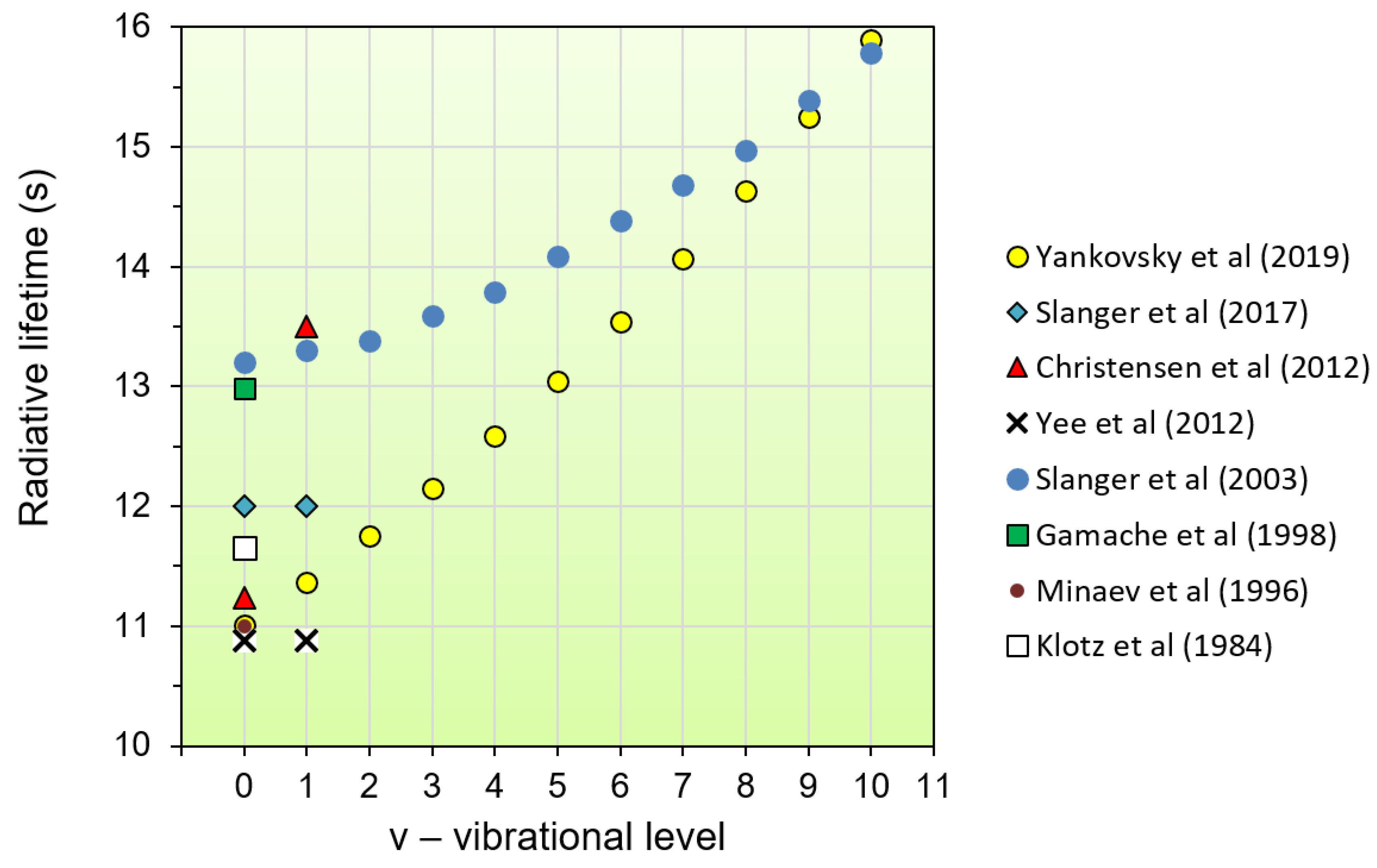
For the first time, new estimates of the radiative lifetimes of electronically–vibrationally excited oxygen molecules O₂(b¹Σ⁺_g, v = 0–10) are presented. These estimates are relevant due to the fact that in the thermosphere, as the height increases, the role of radiation quenching becomes dominant compared to the collisional deactivation (see Section 2.3).

(f)

The model YM2011 allows us to solve both forward and inverse problems. By the forward problem, we mean the calculation of altitude profiles of concentration of excited oxygen components in the MLT region (see Section 4.1). This is especially important for those components whose observations have not yet been implemented. By the inverse photochemical problem, we understand the retrieval of concentrations of non-radiating small atmospheric components that are in the main unexcited state (for example, O(³P), O₃, CO₂) based on the observation of altitude profiles of the emitting singlet levels of oxygen atoms and molecules (see Section 4.2).

The model is continuously developing and enriching itself with new data and fields of application. Currently, the YM2011 model is included in a number of algorithms (GRANADA and ALI-ARMS) and is used for calculations [94]. In the near future, the authors plan to solve the problem of expanding the application of the model for twilight conditions.

References

1. Yankovsky, V.A.; Martyshenko, K.V.; Manuilova, R.O.; Feofilov, A.G. Oxygen dayglow emissions as proxies for atomic oxygen and ozone in the mesosphere and lower thermosphere. J. Mol. Spectrosc. 2016, 327, 209–232. [Google Scholar] [CrossRef]
2. Yankovsky, V.; Vorobeva, E.; Manuilova, R. New techniques for retrieving the [O(3P)], [O3] and [CO2] altitude profiles from dayglow oxygen emissions: Uncertainty analysis by the Monte Carlo method. Adv. Space Res. 2019, 64, 1948–1967. [Google Scholar] [CrossRef]
3. Degen, V. Nightglow emission rates in the O2 Herzberg bands. J. Geophys. Res. 1977, 82, 2437–2438. [Google Scholar] [CrossRef]
4. Llewellyn, E.J.; Solheim, B.H. The excitation of the infrared atmospheric oxygen bands in the nightglow. Planet. Space Sci. 1978, 26, 533–538. [Google Scholar] [CrossRef]
5. Klais, O.; Laufer, A.H.; Kurylo, M.J. Atmospheric quenching of vibrationally excited O2(a1Δg, v). J. Chem. Phys. 1980, 73, 2696–2699. [Google Scholar] [CrossRef]
6. Greer, R.G.H.; Llewellyn, E.J.; Solheim, B.H.; Witt, G. The excitation of the O2(b1Σg+) in the nightglow. Planet. Space Sci. 1981, 29, 383–389. [Google Scholar] [CrossRef]
7. Harris, R.D.; Adams, G.W. Where does the O(1D) energy go? J. Geophys. Res. 1983, 88, 4918–4928. [Google Scholar] [CrossRef]
8. Thomas, R.J.; Young, R.A. Measurement of atomic oxygen and related airglows in the lower thermosphere. J. Geophys. Res. 1981, 86, 7389–7393. [Google Scholar] [CrossRef]
9. Shimazaki, T. The photochemical time constants of minor constituents and their families in the middle atmosphere. J. Atmos. Terr. Phys. 1984, 46, 173–191. [Google Scholar] [CrossRef]
10. McDade, I.C.; Llewellyn, E.J. The excitation of O(1S) and O2 bands in the nightglow: a brief review and preview. Can. J. Phys. 1986, 12, 1626–1630. [Google Scholar] [CrossRef]
11. Clancy, R.T.; Rusch, D.W.; Thomas, R.J.; Allen, M.; Eckman, R.S. Model ozone photochemistry on the basic of solar mesosphere explorer mesospheric observations. J. Geophys. Res. 1987, 92, 3067–3080. [Google Scholar] [CrossRef]
12. Slanger, T.G.; Llewellyn, E.J.; McDade, I.C.; Witt, G. Comment on The O2 atmospheric dayglow in the thermosphere by M. R. Torr, B.Y. Welsh, and D. G. Torr. J. Geophys. Res. 1987, 92, 7753–7755. [Google Scholar] [CrossRef] [Green Version]
13. Evans, W.F.J.; McDade, I.C.; Yuen, J.; Llewellyn, E.J. A rocket measurement of the O2 Infrared Atmospheric (0-0) band emission in the dayglow and a determination of the mesospheric ozone and atomic oxygen densities. Can. J. Phys. 1988, 66, 941–946. [Google Scholar] [CrossRef]
14. Batista, P.P.; Takahashi, H.; Sahai, Y.; Llewellyn, E.J. Mesospheric ozone concentration at an equatorial location from the 1.27 μm O2 airglow emissions. J. Geophys. Res. 1996, 101, 7917–7921. [Google Scholar] [CrossRef]
15. McDade, I.C.; Murtagh, D.P.; Greer, R.G.H.; Dickinson, P.H.G.; Witt, G.; Stegman, J.; Llewellyn, E.J.; Thomas, L.; Jenkins, D.B. ETON 2: quenching parameters for the proposed precursor of O2(b1Σg+) and O(1S) in the terrestrial nightglow. Planet. Space Sci. 1986, 34, 789–800. [Google Scholar] [CrossRef]
16. Murtagh, D.P.; McDade, I.C.; Greer, R.G.H.; Stegman, J.; Witt, G.; Llewellyn, E.J. ETON 4: an experimental investigation of the altitude dependence of the O2(A) vibrational populations in the nightglow. Planet. Space Sci. 1986, 34, 811–817. [Google Scholar] [CrossRef]
17. Greer, R.G.H.; Murtagh, D.P.; McDade, I.C.; Dickinson, P.H.G.; Thomas, L.; Jenkins, D.B.; Stegman, J.; Llewellyn, E.J.; Witt, G.; Mackinnon, D.J.; et al. ETON 1: A database pertinent to the study of energy transfer in the oxygen nightglow. Planet. Space Sci. 1986, 34, 771–788. [Google Scholar] [CrossRef]
18. Grygalashvyly, M.; Eberhart, M.; Hedin, J.; Strelnikov, B.; Lübken, F.-J.; Rapp, M.; Löhle, S.; Fasoulas, S.; Khaplanov, M.; Gumbel, J.; et al. Atmospheric band fitting coefficients derived from a self-consistent rocket-borne experiment. Atmos. Chem. Phys. 2019, 19, 1207–1220. [Google Scholar] [CrossRef] [Green Version]
19. Amaro-Rivera, Y.; Huang, T.-Y.; Urbina, J.; Vargas, F. Empirical values of branching ratios in the three-body recombination reaction for O(1S) and O2(0,0) airglow chemistry. Adv. Space Res. 2018, 62, 2679–2691. [Google Scholar] [CrossRef]
20. Lednyts’kyy, O.; von Savigny, C.; Sinnhuber, M.; Iwagami, N.; Mlynczak, M. Multiple Airglow Chemistry approach for atomic oxygen retrievals on the basis of in situ nightglow emissions. J. Atmos. Sol. Terr. 2019, 194, 105096. [Google Scholar] [CrossRef]
21. Mlynczak, M.G.; Solomon, S.C.; Zaras, D.S. An updated model for O2(a1Δg) concentrations in the mesosphere and lower mesosphere and implications for remote sensing of ozone at 1.27 μm. J. Geophys. Res. 1993, 98, 18639–18648. [Google Scholar] [CrossRef]
22. Torr, M.T.; Torr, D.G. A Preliminary Spectroscopic Assessment of the Spacelab 1/Shuttle Optical Environment. J. Geophys. Res. 1985, 90, 1683–1690. [Google Scholar] [CrossRef]
23. Torr, M.R.; Owens, J.K.; Torr, D.G. Reply [to “Comment on ‘The O2 Atmospheric dayglow in the thermosphere’ by M. R. Torr, B.Y. Welsh, and D. G. Torr”]. J. Geophys. Res. 1987, 92, 7756–7760. [Google Scholar] [CrossRef]
24. Yee, J.-H.; DeMajistre, R.; Morgan, F. The O2(b1Σg+) dayglow emissions: application to middle and upper atmosphere remote sensing. Can. J. Phys. 2012, 90, 769–784. [Google Scholar] [CrossRef]
25. Slanger, T.G.; Copeland, R.A. Energetic Oxygen in the Upper Atmosphere and the Laboratory. Chem. Rev. 2003, 103, 4731–4766. [Google Scholar] [CrossRef] [PubMed]
26. Smith, A.K.; Harvey, V.L.; Mlynczak, M.G.; Funke, B.; Garcia-Comas, M.; Kaufmann, M.; Kyrölä, E.; López-Puertas, M.; McDade, I.; Randall, C.E.; et al. Satellite observations of ozone in the upper mesosphere. J. Geophys. Res. 2013, 118, 5803–5821. [Google Scholar] [CrossRef] [Green Version]
27. Mlynczak, M.G.; Morgan, F.; Yee, J.-H.; Espy, P.; Murtagh, D.; Marshall, B.T.; Schmidlin, F. Simultaneous measurements of the O2(a1Δg) and O2(b1Σg+) airglows and ozone in the daytime mesosphere. Geophys. Res. Lett. 2001, 28, 999–1002. [Google Scholar] [CrossRef]
28. López-Puertas, M.; Taylor, F.W. Non-LTE Radiative Transfer in the Atmosphere; World Scientific Pub.: Singapore, 2001; Volume 3, 487p. [Google Scholar]
29. Park, H.; Slanger, T.G. O2(X, v = 8–22) 300K quenching rate coefficients for O2 and N2, and O2(X) vibrational distribution from 248 nm O3 photodissociation. J. Chem. Phys. 1994, 100, 287–300. [Google Scholar] [CrossRef]
30. Yankovsky, V.A.; Manuilova, R.O. New self-consistent model of daytime emissions of O2(a1Δg, v ≥ 0) and O2(b1Σg+, v = 0, 1, 2) in the middle atmosphere. Retrieval of vertical ozone profile from the measured intensity profiles of these emissions. Atmos. Ocean. Opt. 2003, 16, 536–540. [Google Scholar]
31. Yankovsky, V.A.; Manuilova, R.O.; Kuleshova, V.A. Heating of the middle atmosphere as a result of quenching of the products of O2 and O3 photodissociation. SPIE Proc. Int. Soc. Opt. Eng. 2004, 5743, 34–40. [Google Scholar] [CrossRef]
32. Yankovsky, V.A.; Manuilova, R.O. Model of daytime emissions of electronically-vibrationally excited products of O3 and O2 photolysis: application to ozone retrieval. Ann. Geophys. 2006, 24, 2823–2839. [Google Scholar] [CrossRef] [Green Version]
33. Yankovsky, V.A.; Babaev, A.S. Photolysis of O3 at Hartley, Chappuis, Huggins, and Wulf Bands in the Middle Atmosphere: Vibrational Kinetics of Oxygen Molecules O2(X3Σg, v ≤ 35). Atmos. Ocean. Opt. 2011, 24, 6–16. [Google Scholar] [CrossRef]
34. Yankovsky, V.A.; Manuilova, R.O.; Babaev, A.S.; Feofilov, A.G.; Kutepov, A.A. Model of electronic-vibrational kinetics of the O3 and O2 photolysis products in the middle atmosphere: applications to water vapor retrievals from SABER/TIMED 6.3 μm radiance measurements. Int. J. Remote Sens. 2011, 32, 3065–3078. [Google Scholar] [CrossRef]
35. Yankovsky, V.A.; Manuilova, R.O. Possibility of simultaneous [O3] and [CO2] altitude distribution retrievals from the daytime emissions of electronically-vibrationally excited molecular oxygen in the mesosphere. J. Atmos. Sol. Terr. Phys. 2018, 179, 22–33. [Google Scholar] [CrossRef]
36. Bucholtz, A.; Skinner, W.R.; Abreu, V.J.; Hays, P.B. The dayglow of the O2 atmospheric band system. Planet. Space Sci. 1986, 34, 1031–1035. [Google Scholar] [CrossRef] [Green Version]
37. Mlynczak, M.G.; Marshall, B.T. A reexamination of the role of solar heating in the O2 atmospheric and infrared atmospheric bands. Geophys. Res. Lett. 1996, 23, 657–660. [Google Scholar] [CrossRef]
38. Witt, G.; Stegman, J.; Murtagh, D.P.; McDade, I.C.; Greer, R.G.H.; Dickinson, P.H.G.; Jenkins, D.B. Collisional energy transfer and the excitation of O2(b1Σg+) in the atmosphere. J. Photochem. 1984, 25, 365–378. [Google Scholar] [CrossRef]
39. Torr, M.T.; Torr, D.G. The role of metastable species in the thermosphere. Rev. Geophys. 1982, 20, 91–114. [Google Scholar] [CrossRef]
40. Svanberg, M.; Pettersson, J.B.C.; Murtagh, D. Ozone photodissociation in the Hartley band: A statistical description of the ground state decomposition channel O2(X3Σg) + O(3P). J. Chem. Phys. 1995, 102, 8887–8896. [Google Scholar] [CrossRef]
41. Sparks, R.K.; Carlson, L.R.; Snobatake, K.; Kowalczyk, M.L.; Lee, Y.T. Ozone photolysis: A determination of the electronic and vibrational state distributions of primary products. J. Chem. Phys. 1980, 72, 1401–1402. [Google Scholar] [CrossRef] [Green Version]
42. Valentini, J.J.; Gerrity, D.P.; Phillips, D.L.; Nieh, J.-C.; Tabor, K.D. CARS spectroscopy of O2(a1Δg) from the Hartley band photodissociation of O3: Dynamics of the dissociation. J. Chem. Phys. 1987, 86, 6745–6756. [Google Scholar] [CrossRef]
43. Thelen, M.-A.; Gejo, T.; Harrison, J.A.; Huber, J.R. Photodissociation of ozone in the Hartley band: Fluctuation of the vibrational state distribution in the O2(a1Δg) fragment. J. Chem. Phys. 1995, 103, 7946–7955. [Google Scholar] [CrossRef]
44. Dylewski, S.M.; Geiser, J.D.; Houston, P.L. The energy distribution, angular distribution, and alignment of the O(1D2) fragment from the photodissociation of ozone between 235 and 305 nm. J. Chem. Phys. 2001, 115, 7460–7473. [Google Scholar] [CrossRef] [Green Version]
45. Yankovsky, V.A.; Kuleshova, V.A. Ozone photodissociation at excitation within the Hartley absorption band. Analytical description of quantum yields O2(a1Δg, v = 0–3) depending on the wavelength. Atmos. Ocean. Opt. 2006, 19, 514–518. [Google Scholar]
46. Yankovsky, V.A.; Kuleshova, V.A.; Manuilova, R.O.; Semenov, A.O. Retrieval of total ozone in the mesosphere with a new model of electronic-vibrational kinetics of O2 and O3 photolysis products. Izvestiya Atmos. Ocean. Phys. 2007, 43, 514–525. [Google Scholar] [CrossRef]
47. Martyshenko, K.V.; Yankovsky, V.A. IR Band of O2 at 1.27 μm as the Tracer of O3 in the Mesosphere and Lower Thermosphere: Correction of the Method. Geomagn. Aeron. 2017, 57, 229–241. [Google Scholar] [CrossRef]
48. Klatt, M.; Smith, I.W.M.; Symonds, A.C.; Tuckett, R.P.; Ward, G.N. State-specific rate constants for the relaxation of O2(X3Σg, v = 8–11) in collisions with O2, N2, NO2, CO2, N2O and He. J. Chem. Soc. Faraday Trans. 1996, 92, 193–199. [Google Scholar] [CrossRef]
49. Hernandez, R.; Toumi, R.; Clary, D.C. State-selected vibrational relaxation rates for highly vibrationally excited oxygen molecules. J. Chem. Phys. 1995, 102, 9544–9556. [Google Scholar] [CrossRef]
50. Watanabe, S.; Usuda, S.; Fujii, H.; Hatano, H.; Tokue, I.; Yamasaki, K. Vibrational relaxation of O2(X3Σg, v = 9–13) by collisions with O2. Phys. Chem. Chem. Phys. 2007, 9, 4407–4413. [Google Scholar] [CrossRef]
51. Kalogerakis, K.S.; Copeland, R.A.; Slanger, T.G. Vibrational energy transfer in O2(X3Σg, v = 2, 3) + O2 collisions at 330K. J. Chem. Phys. 2005, 123, 044309. [Google Scholar] [CrossRef]
52. Mack, J.A.; Mikulesky, F.; Wodtke, A.M. Resonant vibration-vibration energy transfer between highly vibrationally excited O2(X, v = 15–26) and CO2, N2O, N2, and O3. J. Chem. Phys. 1996, 105, 4105–4116. [Google Scholar] [CrossRef]
53. Rogaski, C.A.; Price, J.M.; Mack, J.A.; Wodtke, A.M. Laboratory evidence for a possible non-LTE mechanism of stratospheric ozone formation. Geophys. Res. Lett. 1993, 20, 2885–2888. [Google Scholar] [CrossRef]
54. Price, J.M.; Mack, J.A.; Rogaski, C.A.; Wodtke, A.M. Vibrational-state-specific self-relaxation rate constant. Measurements of highly vibrationally excited O2(v = 19–28). Chem. Phys. 1993, 175, 83–98. [Google Scholar] [CrossRef]
55. Coletti, C.; Billing, G.D. Vibrational energy transfer in molecular oxygen collisions. Chem. Phys. Lett. 2002, 356, 14–22. [Google Scholar] [CrossRef]
56. Bloemink, H.I.; Copeland, R.A.; Slanger, T.G. Collisional removal of vibrationally excited O2(b1Σg+) by O2, N2, and CO2. J. Chem. Phys. 1998, 109, 4237–4245. [Google Scholar] [CrossRef]
57. Hwang, E.S.; Bergman, A.; Copeland, R.A.; Slanger, T.G. Temperature dependence of the collisional removal of O2(b1Σg+, v = 1 and 2) at 110–260 K, and atmospheric applications. J. Chem. Phys. 1999, 110, 18–24. [Google Scholar] [CrossRef]
58. Kalogerakis, K.S.; Copeland, R.A.; Slanger, T.G. Collisional removal of O2(b1Σg+, v = 2, 3). J. Chem. Phys. 2002, 116, 4877–4885. [Google Scholar] [CrossRef]
59. Pejakovic, D.A.; Campbell, Z.; Kalogerakis, K.S.; Copeland, R.A.; Slanger, T.G. Collisional relaxation of O2(X3Σg, v = 1) and O2(a1Δg, v = 1) by atmospherically relevant species. J. Chem. Phys. 2011, 135, 094309. [Google Scholar] [CrossRef]
60. Burkholder, J.B.; Abbatt, J.P.D.; Huie, R.E.; Kurylo, M.J.; Wilmouth, D.M.; Sander, S.P.; Barker, J.R.; Kolb, C.E.; Orkin, V.L.; Wine, P.H. Chemical Kinetics and Photochemical Data for Use in Atmospheric Studies: Evaluation Number 18; California Institute of Technology: Pasadena, CA, USA, 2015. [Google Scholar]
61. Yankovsky, V.A. Electron-vibrational relaxation of O2(b1Σg+, v = 1, 2) molecules in collision with ozone, oxygen molecules and atoms. Russ. J. Phys. Chem. 1991, 10, 291–306. [Google Scholar]
62. Esposito, F.; Armehise, I.; Capitta, G.; Capitelli, M. O–O2 state-to-state vibrational-relaxation and dissociation rates based on quasiclassical calculations. Chem. Phys. 2008, 351, 91–98. [Google Scholar] [CrossRef]
63. Dayou, F.; Hernandez, M.I.; Campos-Martinez, J.; Hernandez-Lamoneda, R. Nonadiabatic couplings in the collisional removal of O2(b1Σg+, v) by O2. J. Chem. Phys. 2010, 132, 044313. [Google Scholar] [CrossRef] [PubMed] [Green Version]
64. Klingshirn, H.; Maier, M. Quenching of the 1Σg+ state in liquid isotopes. J. Chem. Phys. 1985, 82, 714–719. [Google Scholar] [CrossRef]
65. Pejakovic, D.A.; Wouters, E.R.; Phillips, K.E.; Slanger, T.G.; Copeland, R.A.; Kalogerakis, K.S. Collisional removal of O2(b1Σg+, v =1) by O2 at thermospheric temperatures. J. Geophys. Res. 2005, 110A, A03308. [Google Scholar] [CrossRef]
66. Torbin, A.P.; Pershin, A.A.; Mebel, A.M.; Zagidullin, M.V.; Heaven, M.C.; Azyazov, V.N. Collisional relaxation of O2(a1Δg, v = 1, 2, 3) by CO2. Chem. Phys. Lett. 2017, 691, 456–461. [Google Scholar] [CrossRef]
67. Wild, E.; Klingshirn, H.; Maier, M. Relaxation of the a1Δg state on pure liquid oxygen and in liquid mixtures of (16)O2 and (18)O2. J. Photochem. 1984, 25, 134–143. [Google Scholar] [CrossRef]
68. Balakrishnan, N.; Dalgarno, A.; Billing, G.D. Multiquantum vibrational transitions in O2(v≥25) + O2(v=0) collisions. Chem. Phys. Lett. 1998, 288, 657–662. [Google Scholar] [CrossRef]
69. Billing, G.D. VV and VT rates in N2–O2 collisions. Chem. Phys. 1994, 179, 463–467. [Google Scholar] [CrossRef]
70. Sharma, R.D.; Welsh, J.A. Vibrational energy transfer in O2(v = 2–8)–O2(v = 0) collisions. J. Chem. Phys. 2009, 130, 194306. [Google Scholar] [CrossRef]
71. Yu, S.; Drouin, B.J.; Miller, C.E. High resolution spectral analysis of oxygen. IV. Energy levels, partition sums, band constants, RKR potentials, Franck-Condon factors involving the X3Σg, a1Δg and b1Σg+ states. J. Chem. Phys. 2014, 141, 174302. [Google Scholar] [CrossRef]
72. Nicholls, R.W. Franck-Condon Factors to High Vibrational Quantum Numbers V: O2 Band Systems. J. Res. Natl. Bur. Stand. Sect. Phys. Chem. 1965, 69A, 369–373. [Google Scholar] [CrossRef]
73. Krupenie, P.H. The spectrum of molecular oxygen. J. Phys. Chem. Ref. Data 1972, 1, 423–521. [Google Scholar] [CrossRef] [Green Version]
74. Minaev, B.F. Magnetic phosphorescence of molecular oxygen. A study of the b–X transition probability using multiconfiguration response theory. Chem. Phys. 1996, 208, 299–311. [Google Scholar] [CrossRef]
75. Brown, L.R.; Plymate, C. Experimental line parameters of oxygen A band at 760 nm. J. Mol. Spectrosc. 2000, 199, 166–179. [Google Scholar] [CrossRef] [PubMed] [Green Version]
76. Gamache, R.R.; Goldman, A. Einstein A coefficient, integrated band intensity, and population factors: application to the a1Δg–X3Σg (0, 0) O2 band. J. Quantative Spectrosc. Radiat. Transf. 2001, 69, 389–401. [Google Scholar] [CrossRef]
77. Goldman, A.; Stephen, T.V.; Rothman, L.S.; Giver, L.P.; Mandin, J.-Y.; Gamache, R.R.; Rinsland, C.P.; Murcray, F.J. The 1-μm CO2 bands and the O2(0-1) X3Σg–a1Δg and (1-0) X3Σgb1Σg+ bands in the Earth atmosphere. J. Quantative Spectrosc. Radiat. Transf. 2003, 82, 197–205. [Google Scholar] [CrossRef]
78. Gordon, I.E.; Rothman, L.S.; Toon, G.C. Revision of spectral parameters for the B- and g-bands of oxygen and their validation against atmospheric spectra. J. Quantative Spectrosc. Radiat. Transf. 2011, 112, 2310–2322. [Google Scholar] [CrossRef]
79. Long, D.A.; Hodges, J.T. On spectroscopic models of the O2 A-band and their impact upon atmospheric retrievals. J. Geophys. Res. 2012, 117, D12309. [Google Scholar] [CrossRef]
80. Naus, H.; Ubachs, W. The b1Σg+–X3Σg (3, 0) band of (16)O2 and (18)O2. J. Mol. Spectrosc. 1999, 193, 442–445. [Google Scholar] [CrossRef] [Green Version]
81. Rothman, L.S.; Rinsland, C.P.; Goldman, A.; Massie, S.T.; Edwards, D.P.; Flaud, J.M.; Schroeder, J. The HITRAN molecular spectroscopic database and hawks (HITRAN atmospheric workstation): 1996 Edition. J. Quantative Spectrosc. Radiat. Transf. 2010, 60, 665–710. [Google Scholar] [CrossRef]
82. Kuznetsova, L.A.; Kuzmenko, N.E.; Kuziakov, I.I.; Plastinin, I.A. Probabilities of Optical Transitions of Diatomic Molecules; Soviet Phys. Uspekhi. ed.; NAUKA: Moscow, Russia, 1980; 320p. (In Russian) [Google Scholar]
83. Kassi, S.; Romanini, D.; Campargue, A.; Bussery-Honvault, B. Very high sensitivity CW-cavity ring down spectroscopy: Application to the a1Δg(0)–X3Σg(1) O2 band near 1.58 μm. Chem. Phys. Lett. 2005, 409, 281–287. [Google Scholar] [CrossRef]
84. Gamache, R.R.; Goldman, A.; Rothman, L.S. Improved spectral parameters for the three most abundant isotopomers of the oxygen molecule. J. Quantative Spectrosc. Radiat. Transf. 1998, 59, 495–509. [Google Scholar] [CrossRef]
85. Christensen, A.B.; Yee, J.-H.; Bishop, R.L.; Budzien, S.A.; Hecht, J.H.; Sivjee, G.; Stephan, A.W. Observations of molecular oxygen Atmospheric band emission in the thermosphere using the near infrared spectrometer on the ISS/RAIDS experiment. J. Geophys. Res. 2012, 117, A04315. [Google Scholar] [CrossRef] [Green Version]
86. Slanger, T.G.; Pejakovic, D.A.; Kostko, O.; Matsiev, D.; Kalogerakis, K.S. Atmospheric dayglow diagnostics involving the O2(b–X) Atmospheric band emission: Global Oxygen and Temperature (GOAT) mapping. J. Geophys. Res. Space Phys. 2017, 122, 3640–3649. [Google Scholar] [CrossRef]
87. Klotz, R.; Marian, C.M.; Peyrimhoff, S.D.; Hess, B.A.; Buenker, R.J. Calculation of spin-forbidden radiative transitions using correlated wavefunctions: lifetimes of b, a states in O2, S2 and SO. Chem. Phys. 1984, 89, 223–236. [Google Scholar] [CrossRef]
88. Slanger, T.G.; Black, G. O(1S) in the lower thermosphere—Chapman vs. Barth. Planet. Space Sci. 1977, 25, 79–88. [Google Scholar] [CrossRef]
89. Wu, K.; Fu, D.; Feng, Y.; Li, J.; Hao, X.; Li, F. Simulation and application of the emission line O19P18 of O2(a1Δg) dayglow near 1.27 μm for wind observations from limb-viewing satellites. Opt. Express 2018, 26, 16984–16999. [Google Scholar] [CrossRef]
90. Atkinson, R.; Baulch, D.L.; Cox, R.A.; Crowley, J.N.; Hampson, R.F.; Hynes, R.G.; Jenkin, M.E.; Rossi, M.J.; Troe, J. Evaluated kinetic and photochemical data for atmospheric chemistry: Volume I–gas phase reactions of Ox, HOx, NOx and SOx species. Atmos. Chem. Phys. 2004, 4, 1461–1738. [Google Scholar] [CrossRef] [Green Version]
91. Balakrishnan, N.; Billing, G.D. Quantum-classical reaction path study of the reaction O(3P) + O3(1A1) → 2 O2(X3Σg). J. Chem. Phys. 1996, 104, 9482–9494. [Google Scholar] [CrossRef]
92. SABER—Sounding of the Atmosphere Using Broadband Emission Radiometry. Available online: http://saber.gats-inc.com/data.php (accessed on 19 January 2020).
93. SORCE. Available online: http://science.nasa.gov/missions/sorce/ (accessed on 19 January 2020).
94. He, W.; Wu, K.; Feng, Y.; Fu, D.; Chen, Z.; Li, F. Radiative Transfer Characteristics of the O2 Infrared Atmospheric Band in Limb-Viewing Geometry. Remote Sens. 2019, 11, 2702. [Google Scholar] [CrossRef] [Green Version]
Figure 1. Block-scheme of electronically–vibrationally excited oxygen molecules formation in the daytime mesosphere and lower thermosphere. Red solid lines represent products of O2 and O3 photolysis, black solid lines show energy transfer as a result of collisional reactions, wave arrows correspond to emission transitions.
Atmosphere 11 00116 g001
Figure 2. Quantum yields of O2(X3Σg, v = 0–35) formation in the triplet channel of ozone photolysis depending on wavelength [40]. Colors correspond to subintervals of quantum yield values: violet (0.00–0.03), dark red (0.03–0.06), yellow (0.06–0.09), blue (0.09–0.12), purple (0.12–0.15).
Atmosphere 11 00116 g002
Figure 3. Quantum yields of O2(a1Δg, v = 0–5), which are produced in result of the O3 photolysis in Hartley band. Experimental data: violet triangles (v = 0), green crosses (v = 1), orange squares (v = 2), blue circles (v = 3), red pluses (v = 4) and black diamond (v = 5). Calculations by Equations (3) and (4) for different v are solid lines with corresponding colors.
Atmosphere 11 00116 g003
Figure 4. Rate coefficients of O2(X3Σg, v) + O2 → products [29,32,48,50,51,52,53,54,55] and O2(X3Σg, v) + N2 → products [29] depending on module of energy mismatch. The numbers indicate values of the vibrational quantum.
Atmosphere 11 00116 g004
Figure 5. The same as Figure 4 but for O2(b1Σg+, v) + O2 → products (blue circles), O2(b1Σg+, v) + N2 → products (blue squares), O2(b1Σg+, v) + O3 → products (blue diamonds), O2(a1Δg, v) + O2 → products (red circles), O2(a1Δg, v) + O3 → products (red diamonds) [2].
Atmosphere 11 00116 g005
Figure 6. Rate coefficients of O2(X3Σg, v ≤ 30) + O(3P) → O2(X3Σg, v′ = v − Δv) + O(3P) depending on v and v′ [62].
Atmosphere 11 00116 g006
Figure 7. Currently known estimations of O2(b1Σg+, v = 0–10) radiative lifetimes [2,24,25,74,84,85,86,87].
Atmosphere 11 00116 g007
Figure 8. Left panel: altitude profiles of O(3P) concentration for different latitudes from TIMED-SABER data (day 172, year 2010). Right panel: the contribution of the Barth’ mechanism to the O2(b1Σg+, v = 0) excitation with respect to the photolytic excitation mechanism of O2(b1Σg+, v = 0) in the framework of YM2011 model. Three sets of parametric coefficients for the Barth’ mechanism were used in the calculation (see legend) [15,18,19].
Atmosphere 11 00116 g008
Figure 9. The block-diagram of the population of O2(X3Σg, v = 1–35) levels in the mesosphere and lower thermosphere, according to YM2011 model (version 2019). A brief notation of levels: O2(X, v) = O2(X3Σg, v), O2(a, v) = O2(a1Δg, v), O2(b, v) = O2(b1Σg+, v). Direct sources of formation of O2(X, v) molecules are photolysis of ozone in the Hartley, Huggins, Chappuis, and Wulf bands (blue triangle), the reaction O3 + O(3P) → O2(X, v ≤ 30) + O2 (brown rhombus). The dashed-dotted line indicates the quasi-resonant EE’ energy transfer as a result of O2(b, 0) + O2 → O2(a, v) + O2(X, 3-v); long-dashed lines denote quasi-resonant EV energy transfer as a result of O2(a, 0) + O2 → O2(X, v) + O2(X, 5-v); red inclined lines—quasi-resonant EV exchange as a result of O2(a, v) + O2 → O2(X, v) + O2(a, 0) and O2(b, v) + O2 → O2(X, v) + O2(b, 0) for the first and second singlet states of the oxygen molecule. The black vertical arrows are the relaxation processes of the O2(X, v) levels in the reactions O2(X, v) + O2 → O2(X, v-1) + O2(X, 1), O2(X, v) + O2 → O2(X, v-1) + O2(X, 0), O2(X, v) + O(3P) → O2(X, v-Δv) + O(3P) and O2(X, v) + N2 → O2(X, v-2) + N2(X, 1). The wide non-solid arrow for O2(X, 1) denotes VT quenching of O2(X, 1) + M → O2(X, 0) + M, where M = O2, N2, O(3P). The quasi-resonant reactions that we hypothesized are indicated by curved lines: violet is for the reaction O2(b, 0) + N2 → O2(X, 9) + N2, yellow is for the reaction O2(b, 1) + O(3P) → O2(X, 10) + O(3P) (see Table 2).
Atmosphere 11 00116 g009
Figure 10. Population of O2(X3Σg, v = 1–35) levels for altitude from 50 to 120 km. Calculation using YM2011 model for TIMED-SABER event (37_01468), Date 16.03.2002, Lat = 43.3, SZA = 50.0.
Atmosphere 11 00116 g010
Figure 11. Altitude distributions of O2(X3Σg, v = 1) (solid curve) and O2(X3Σg, v = 2) (dashed curve) depending on solar zenith angle. Calculation is for SABER events during the vernal equinox 2002 using YM2011 model.
Atmosphere 11 00116 g011
Figure 12. The scheme of electronic–vibrational kinetics of the products of O2 and O3 photolysis in the MLT region (YM2011 model, version 2019), taking into account 9 excited levels of the oxygen molecule (three levels O2(b1Σ+g, v = 0, 1, 2), six levels O2(a1Δg, v = 0–5)), 35 levels O2(X3Σg, v = 1–35) and, also, the excited level of the oxygen atom, O(1D). Solid thin lines with arrows designate the processes of O2 and O3 photolysis. Double vertical lines with arrows designate the processes of solar radiation resonance absorption in the 762 nm (gα), 688 nm (gβ), 629 nm (gγ) and in the 1.27 µm (gIRa) bands. Short dashed inclined lines with arrows present energy transfer from O(1D) to the O2(b1Σ+g, v = 0, 1), from O2(b1Σ+g, v = 0) to O2(a1Δg, v = 0–3) and from O2(a1Δg, v = 0) to O2(X3Σ¯g, v = 0–5) at collisional quenching. Long dashed vertical lines with arrows denote collisional V–V transitions. Solid orange vertical lines with arrows pointed down designate the processes of emissions from electronic–vibrational levels of O2 molecule and from excited atom O(1D).
Atmosphere 11 00116 g012
Figure 13. Daily mean altitude profiles of O2(b1Σg+, v = 0) (blue solid line), O2(b1Σg+, v = 1) (green solid line), O2(b1Σg+, v = 2) (red solid line), O(1D) (black solid line) and their standard deviations (dashed lines) calculated via YM2011 based on TIMED-SABER data for 4 days in 2010: (a) day 79, (b) day 172, (c) day 265, (d) day 355. Orange lines represent altitude profiles of O(1D) according to TIMED-SABER data.
Atmosphere 11 00116 g013