Article

A Markov Chain-Based Bias Correction Method for Simulating the Temporal Sequence of Daily Precipitation

1
State Key Laboratory of Water Resources and Hydropower Engineering Science, Wuhan University, Wuhan 430072, China
2
Hubei Key Laboratory of Water System Science for Sponge City Construction (Wuhan University), Wuhan 430010, China
3
USDA-ARS Grazinglands Research Lab., 7207 West Cheyenne St., E1 Reno, OK 73036, USA
4
Department of Geosciences, University of Oslo, P.O, Box 1047, Blindern, 0316 Oslo, Norway
5
Changjiang Institute of Survey, Planning, Design and Research, Wuhan 430010, China
*
Author to whom correspondence should be addressed.
Atmosphere 2020, 11(1), 109; https://doi.org/10.3390/atmos11010109
Submission received: 31 October 2019 / Revised: 8 January 2020 / Accepted: 11 January 2020 / Published: 16 January 2020
(This article belongs to the Special Issue Climate Data for Agricultural Applications: Downscaling and Scenarios)

Abstract

:
Bias correction methods are routinely used to correct climate model outputs for hydrological and agricultural impact studies. Even though superior bias correction methods can correct the distribution of daily precipitation amounts, as well as the wet-day frequency, they usually fail to correct the temporal sequence or structure of precipitation occurrence. To solve this problem, we presented a hybrid bias correction method for simulating the temporal sequence of daily precipitation occurrence. We did this by combining a first-order two-state Markov chain with a quantile-mapping (QM) based bias correction method. Specifically, a QM-based method was used to correct the distributional attributes of daily precipitation amounts and the wet-day frequency simulated by climate models. Then, the sequence of precipitation occurrence was simulated using the first-order two-state Markov chain with its parameters adjusted based on linear relationships between QM-corrected mean monthly precipitation and the transition probabilities of precipitation occurrence. The proposed Markov chain-based bias correction (MCBC) method was compared with the QM-based method with respect to reproducing the temporal structure of precipitation occurrence over 10 meteorological stations across China. The results showed that the QM-based method was unable to correct the temporal sequence, with the cumulative frequency of wet- and dry-spell length being considerably underestimated for most stations. The MCBC method can could reproduce the temporal sequence of precipitation occurrence, with the generated cumulative frequency of wet- and dry-spell lengths fitting that of the observation well. The proposed method also performed reasonably well with respect to reproducing the mean, standard deviation, and the longest length of observed wet- and dry-spells. Overall, the MCBC method can simulate the temporal sequence of precipitation occurrence, along with correcting the distributional attributes of precipitation amounts. This method can be used with crop and hydrological models in climate change impact studies at the field and small watershed scales.

1. Introduction

As an essential part of the third working group report from the Intergovernmental Panel on Climate Change’s (IPCC, 2018) sixth assessment report, food security under climate change conditions plays a vital role in the survival and development of human beings. Thus, it is vital to accurately assess the climate change on site-specific or small catchment scales for adopting adaptation strategies to mitigate the negative effect of climate change on agricultural production. Global climate models (GCMs) are primary tools for studying the impacts of climate change on agriculture and hydrology, as well as other fields [1,2,3,4]. However, the resolution of GCM outputs is too coarse to be used as direct inputs into agricultural and hydrological models for site-specific and watershed climate change impact studies [5,6,7,8,9]. In addition to the spatial mismatch, the biases deriving from the systematic error, such as imperfect model specification, also hinder the direct use of GCM simulations for impact studies [10,11,12,13]. Dynamical downscaling, which involves nesting the regional climate model (RCM) with the initial and time-dependent lateral boundary condition of GCMs by dynamical formulations [5,9,10,14,15,16], has been developed to solve these problems. Although RCMs usually perform better than GCMs in simulating climate at the regional scale, the resolution is still too coarse and the simulation is still biased to be used for local and site-specific impact studies [10,17,18,19].
Bias correction methods are commonly used to post-process RCM and GCM simulations before driving the agricultural and hydrological models for impact studies. When observations have a similar spatial resolution (gridded data) to climate model outputs, bias correction methods correct the bias of the climate model outputs. While the spatial resolution of climate model outputs is coarser than that of the observations, the bias correction method serves as both downscaling and bias correction. A large number of bias correction methods have been developed during the last two decades. They range from simple mean-based methods to sophisticated distribution-based quantile mapping methods, and from single-site approaches to multisite and multivariate approaches [5,6,20,21,22]. The mean-based method corrects the multiple-year mean of a climate model simulation based on the difference between the mean of the climate model simulation and that of the observation in the reference period. The distribution-based method corrects the distribution of climate model simulations. Given the ease of application and the reasonable performance, bias correction becomes the standard process when using climate model outputs for impact studies [19,23,24,25,26].
Bias correction methods usually perform well in correcting the distributional attributes of climate model outputs (e.g., precipitation and temperature). In particular, the distribution-based methods usually perform better than the mean-based methods. For example, Teutschbein and Seibert [22] compared five bias correction methods in correcting RCM-simulated temperature and precipitation in terms of evaluating the hydrological climate change impacts over five catchments in Sweden. The results showed that all bias correction methods could reduce the bias of RCM simulations and the distribution-based methods generally performed better than the mean-based methods.
In addition to correcting the distributional attributes of climate variables, some superior bias correction methods also correct the wet-day frequency of precipitation [10,27]. For example, Themeßl et al. [28] proposed an empirical distribution mapping method, which corrects the wet-day frequency along with the correction of the empirical cumulative distribution function of precipitation amounts. Bias correction methods usually correct the wet-day frequency by finding a precipitation threshold to ensure that the wet-day frequency of corrected data is equal to that of the observation in the reference period [29]. The same precipitation threshold is used for the future period. However, all these bias correction methods do not consider the correction of the temporal sequence of precipitation occurrence (i.e., wet- and dry-spells) [6,21,30,31,32,33], which may result in biased hydrological simulations [21].
The temporal sequence of precipitation occurrence is essential for hydrological simulations over small watersheds and crop production modeling at the field scale. For example, the unordered temporal sequence of precipitation occurrence may result in biased runoff and soil water dynamics simulated by a hydrological model, even though the total monthly precipitation amount is the same [11]. The temporal sequence of precipitation occurrence can be simulated using stochastic models, such as a Markov chain [19,34,35,36,37,38,39,40,41]. For example, Apipattanavis et al. [42] used a Markov chain-based model to simulate the precipitation occurrence over Pergamino in Argentina, and they found that the Markov chain was capable of capturing the statistics of all the spells. Zhang [19] validated a Markov chain-based model in reproducing the precipitation series at five stations in Oklahoma, where they found that the sequence of the observed precipitation was well reproduced by this method for all stations. The Markov chain-based model is usually incorporated into weather generators to simulate the temporal sequence of precipitation occurrence. When using the weather generator as a downscaling tool, its parameters need to be adjusted based on climate change information between future and historical periods. However, the adjustment of weather generator parameters is not an easy task, especially for downscaling precipitation occurrence.
This study proposes a hybrid bias correction method by combining a commonly used bias correction method (i.e., the daily bias correction method, DBC) with the first-order two-state Markov chain. The new method takes advantage of the traditional bias correction method in correcting the distributional attributes of precipitation amounts and wet-day frequency, and it takes advantage of the Markov chain in simulating the sequence of precipitation occurrence. The performance of the proposed Markov-chain based bias correction method (MCBC) is evaluated using comparisons to the DBC over 10 stations across China.

2. Study Area and Data Sources
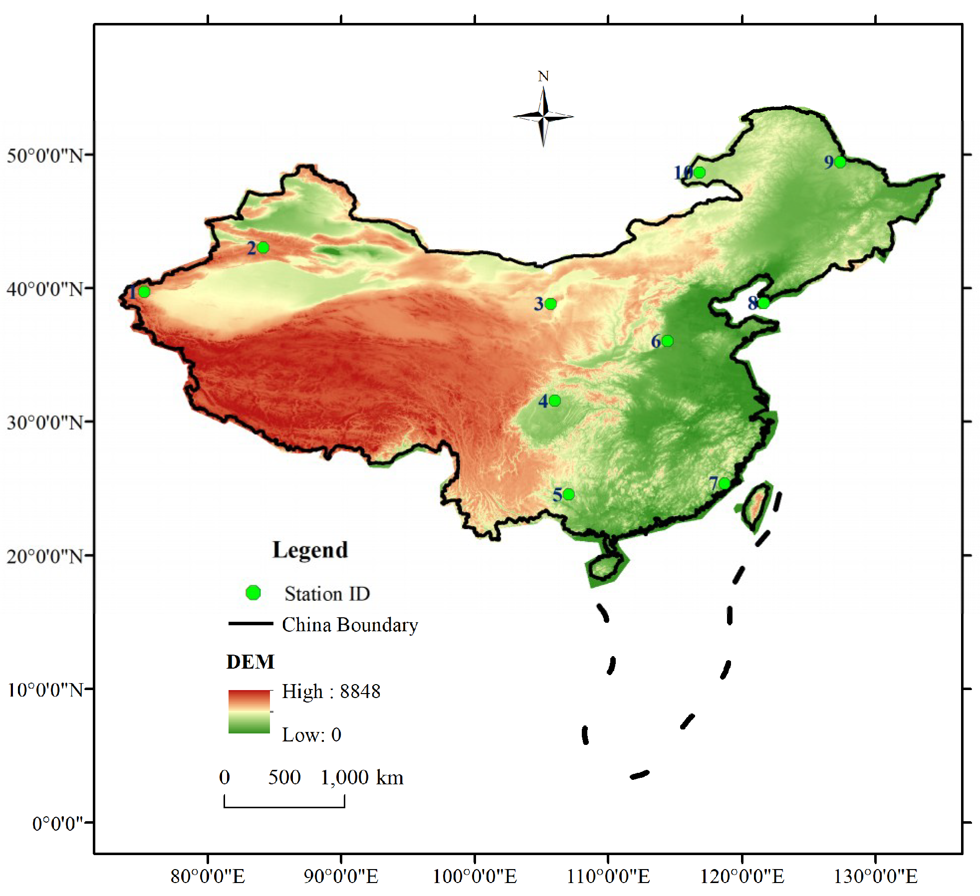
2.1. Study Area

The performance of the proposed bias correction was demonstrated using ten meteorological stations distributed across different climatic zones in China (Figure 1). The mean annual precipitation at these stations ranged from 185 mm to 1565 mm, with the wet day frequency varying from 15% to 44%. The detailed information, including longitude, latitude, and elevation for the ten stations, can be found in Table 1.

2.2. Data Sources

This study used both the observed and GCM-simulated precipitation. The observed precipitation series of 10 meteorological stations were obtained from the China Meteorological Data Sharing Service System (http://data.cma.cn/data/index/0b9164954813c573.html), covering the 1961–2014 period. Precipitation simulated by the 10 GCMs was extracted from the Coupled Model Inter-comparison Project Phase 5 (CMIP5) database. Table 2 shows the detailed information of these GCMs. The grid box that overlaps the observed gauge was selected to represent the simulated precipitation for this station. All simulated precipitation time series cover the 1961–2005 period.

3. Methodology

The proposed bias correction method is a two-stage hybrid method combining the quantile-mapping (QM) method with the first-order two-state Markov chain. The first stage involves correcting the distribution of precipitation amounts on wet days and the wet-day frequency of the projected GCM-simulated precipitation using the QM-based method by Chen et al. [5]. This bias correction method is conceptually simple and widely used [10,21,29,43,44]. The second stage involves generating the temporal sequence of precipitation occurrence using the first-order two-state Markov chain based on the first stage corrected monthly precipitation amounts. More details of this method are described as follows.

3.1. Quantile Mapping Bias Correction Method

The QM method used in this study is the DBC method [10], which is a combination of the daily translation (DT) [45] and local intensity scaling (LOCI) methods [27]. The DBC method inherits the merit of the LOCI method in correcting the wet-day frequency of precipitation occurrence and that of the DT method in correcting the frequency distribution of precipitation amounts. Specifically, for each calendar month, the LOCI method first determines a threshold for the GCM-simulated precipitation time series so that the wet-day frequency of simulated precipitation series for the calibration period is equal to that of the observed precipitation. Then, different scaling factors, which are the ratios in percentiles between the observed and climate model-simulated precipitation in the calibration period, are applied to the corresponding percentiles in the validation period. One hundred percentiles are used to represent the frequency distribution of the precipitation amounts. All bias correction methods assume that the biases of climate model simulations are stationary over time, which means that the biases of climate model simulations at the calibration period do not change at the validation period. Even though the distribution of precipitation at the validation period may differ from that at the calibration period, the same biases can be removed. The formulation of DBC for correcting the distribution of precipitation is presented as follow:
P c o r , c a l i , m , p = P o b s , m , p P c a l i , m , p P c a l i , m , p ,
P c o r , v a l i , m , p = P o b s , m , p P c a l i , m , p P v a l i , m , p ,
The subscripts obs, cali, and vali denote the observation, calibration period, and validation periods; and m and P denote the months and percentile, respectively, while cor denotes corrected data.

3.2. The First-Order Two-State Markov Chain

The first-order two-state Markov chain is widely used to simulate the sequence of precipitation, and its consistent performance has been demonstrated in many studies [6,34,46,47]. When using this method, the probability of precipitation on a given day is determined based on the precipitation status (dry or wet) of a previous day. The transition probability P11 is the probability of a wet day following a wet day, and P01 is the probability of a wet day following a dry day, as shown in the following formulas:
P01 = Pr {precipitation on day t | no precipitation on day t − 1}
P11 = Pr {precipitation on day t | precipitation on day t − 1}
Given the status of a previous day, for example, a dry day, if a random number derived from a standard uniform distribution is less than P01, a wet day is generated; and otherwise, a dry day is generated. A similar process can also be used with P11.

3.3. Hybrid Bias Correction Method

When using the first-order, two-state Markov chain to simulate the temporal sequence of precipitation occurrence, P01 and P11 must be adjusted according to the climate change signal simulated by the climate models. Previous studies showed that there are strong linear relationships between the mean monthly precipitation and the two conditional transition probabilities [16,19,30]. The linear relationship can be fitted using the observed precipitation time series. In other words, if we know the mean monthly precipitation of the validation period, two conditional transition probabilities for this period can be obtained based on the linear relationship established in the calibration period. As mentioned earlier, the QM method can provide an accurate simulation of the monthly precipitation amounts.
A linear relationship between the transition probabilities of precipitation occurrence and the mean monthly precipitation is first established using the four-point regression method of Zhang et al. [16]. The method is based on the observed precipitation time series, as in the following three steps.
(a)
Taking January as an example, the total precipitation of this month over the whole period is sorted in ascending order and then separated into dry and wet groups. Then the mean monthly precipitation is calculated from each group. The daily series corresponded to the months in each group are gathered and used to calculate P01 and P11. With this step, a set of P01, P11, and the mean monthly precipitation is calculated for each group.
(b)
The total precipitation of this month each year is also divided into two, even periods in chronological order. A set of parameters is also calculated for each period.
(c)
A linear equation is established for P01 (and P11) and the mean monthly precipitation based on the four samples calculated from step-(a) and step-(b).
The use of two extreme cases (the sorted dry and wet conditions) of precipitation occurrence versus the amounts is done to ensure that the fitted relationship can hold for the changing climate. In other words, including the two extreme cases in establishing the linear relationship implicitly incorporates non-stationary climate conditions when estimating the transition probabilities of precipitation occurrence for any climatic conditions within the entire range. With the bias-corrected mean monthly precipitation for the validation period, the transition probabilities P01 and P11 can be regressed using the established linear relationships for each calendar month. The first-order, two-state Markov chain is used to generate the sequence of precipitation occurrence. For a predicted wet day, the precipitation amount is generated by realigning the DBC-corrected precipitation amounts. Specifically, a set of random numbers is first generated for wet days simulated by the first-order, two-state Markov chain. The random numbers are then replaced by DBC-corrected precipitation amounts, according to the numerical value of the random number. In other words, the larger precipitation amount is given to the larger random number, and vice versa. If the first-order, two-state Markov chain is perfect for simulating the sequence of precipitation occurrence, then the simulated wet- and dry-day frequencies should be equal to the frequencies generated by the DBC. However, this may not be the case. Scaling the realigned daily precipitation for each month may be necessary to correct or offset the generation error of the first-order, two-state Markov chain. This is done by multiplying the ratio of the DBC-corrected mean monthly precipitation and MCBC-corrected mean monthly precipitation by the daily precipitation series of the MCBC-sampled for each specific month.

3.4. Analysis Procedure And Statistics

The performance of the proposed hybrid method was validated based on the observed and GCM-simulated precipitation time series from 1961 to 2005. Before evaluating the MCBC method, its baseline model is demonstrated using 10 stations in China, i.e., the performance of the DBC method and the linear relationships between the mean monthly precipitation and conditional probabilities of precipitation occurrence. A split-sample cross-validation method was conducted to evaluate the performance of the DBC method [8]. Specifically, the time series of the observation and GCM simulations for the 1961–2005 period is divided into five equal sub-periods (1961–1969, 1970–1978, 1979–1987, 1988–1996, and 1997–2005). Four sub-periods are used to calibrate the DBC method and the remaining sub-period is used for validation. The above processes are conducted five times to get five validation sub-periods. The five validation sub-periods are then combined to get a 45-year validation period. The data length used in the calibration of the linear relationships between the mean monthly precipitation and the conditional probabilities of precipitation occurrence was more than 90 years in prior studies by Zhang et al. [16,19]. Owing to the limited data length, we conducted this process with the total observations from 1961–2014.
The Markov chain-based bias correction (MCBC) method was applied to correct the daily precipitation series simulated by the climate models for each station. The nonparametric two-sample Kolmogorov–Smirnov (K-S) test was used to test whether the bias-corrected and observed precipitations were from the same distribution. The same method has been used in many other studies [16,19,30,35]. The statistical test D was calculated from the length of the two tested samples and the null hypothesis was that the two samples were from the same distribution. When the maximum deviation between the cumulative frequency distribution of two samples was larger than D at the 0.05 significance level, the null hypothesis was rejected, and vice versa.

4. Results

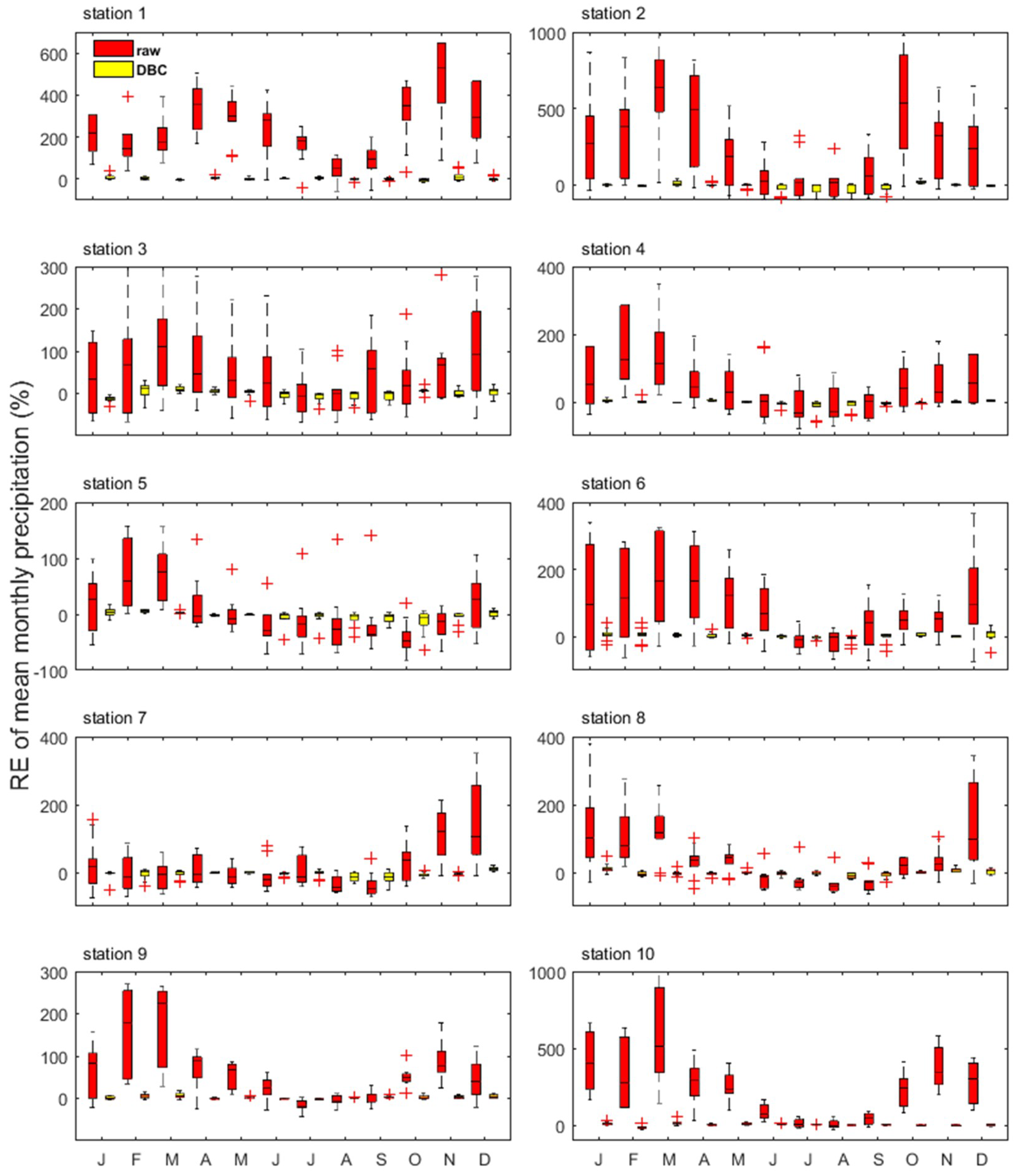
4.1. Validation of the Daily Bias Correction

The performance of the DBC method for bias correcting GCM precipitation has been verified in many studies [21,29]. Since the premise of the MCBC method is to obtain the well-corrected mean monthly precipitation used to interpolate the conditional transition probabilities, only the performance of the DBC method in correcting the mean monthly precipitation is demonstrated in Figure 2.
The raw GCMs considerably overestimated the mean monthly precipitation, with the medians of the relative errors (REs) ranging between 50% and 300% for most stations and months. In terms of the RE, the simulated mean monthly precipitations in July, August, and September are slightly better than in other months for most stations. The result was because most stations had higher precipitation in these three months than in other months. The biases of the mean monthly precipitation simulated by the GCMs were largely reduced by the DBC method. For example, the medians of REs across all GCMs ranged between 0.01% and 14.7%, and these errors were due to cross-validation. Although the performance of the DBC method partly depends on a specific month and location, it generally corrects the mean monthly precipitation for all GCMs accurately.

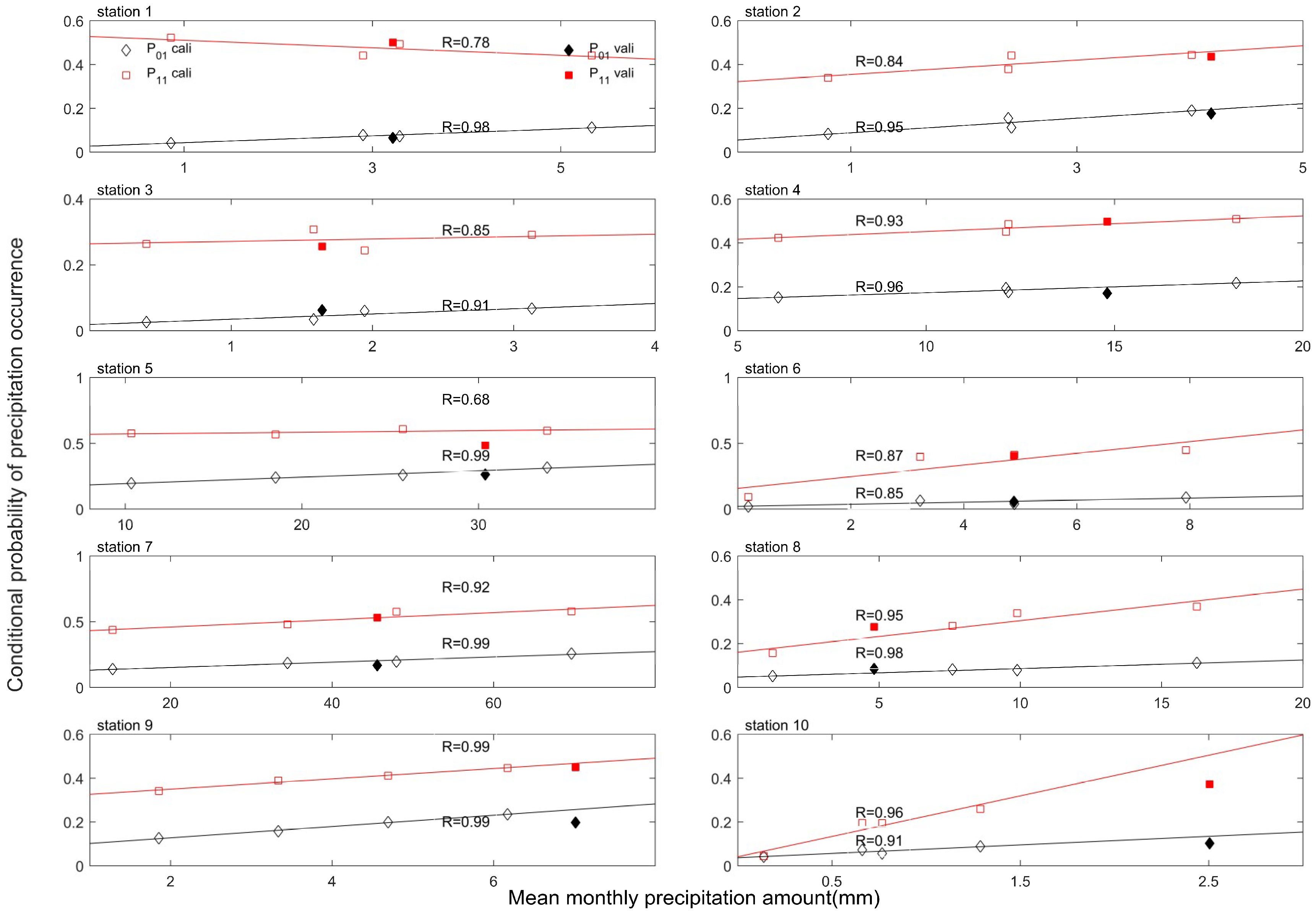
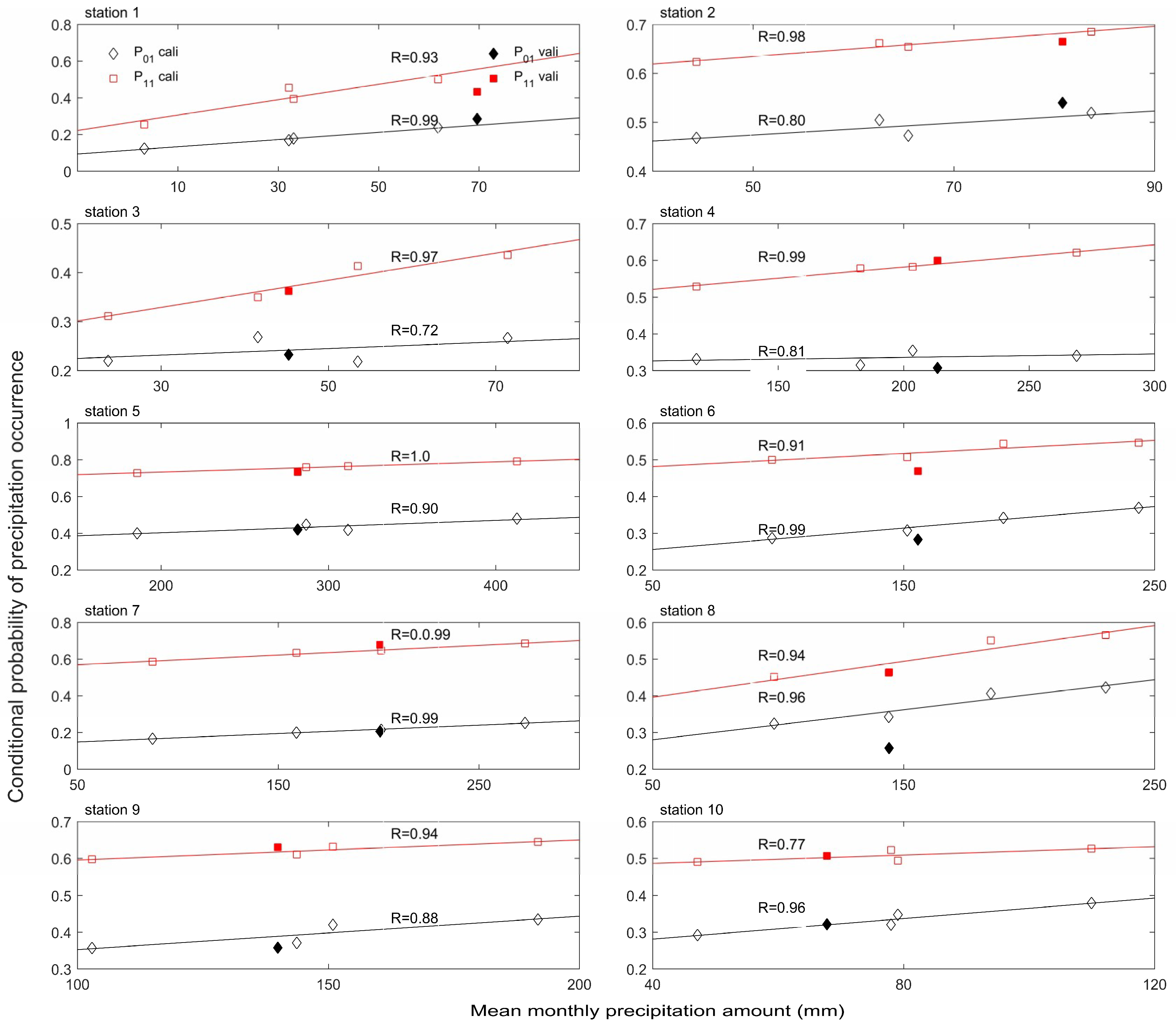
4.2. Validation of the Linear Relationships

The data points of P01, P11, and mean monthly precipitation, which were calculated from the dry group, wet group, and two even groups of the calibration period, are plotted in Figure 3 and Figure 4 for January and July, respectively for the ten stations. The linear curves that were regressed using the four data points were used to interpolate the conditional transition probabilities in the validation period. For comparison, P01, P11, and the mean monthly precipitation were also calculated for the validation period and plotted in Figure 3 and Figure 4 as solid points. The names of the legend ‘cali’ and ‘vali’ represent calibration and validation, respectively.
Overall, the regression lines fitted the data points very well for all months and stations, indicating a strong linear relationship between the mean monthly precipitation and conditional transition probabilities. In particular, the data points of P01 from both the calibration and validation periods were fairly close to the regression lines. The correlation coefficient between mean monthly precipitation and transition probabilities was greater than 0.9 for 91 out of 120 cases (12 months × 10 stations) for P01, and for 75 out of 120 cases for P11. The reason why there was a stronger relationship for P01 than P11 may be because the occurrence of wet-following-wet events is lesser than that of wet-following-dry events, which contributed to greater variability and less reliability when estimating P11. As Zhang et al. (2012) presented in their study that a longer period should be used to obtain large samples of wet-following-wet events to improve the accuracy of the estimated P11.

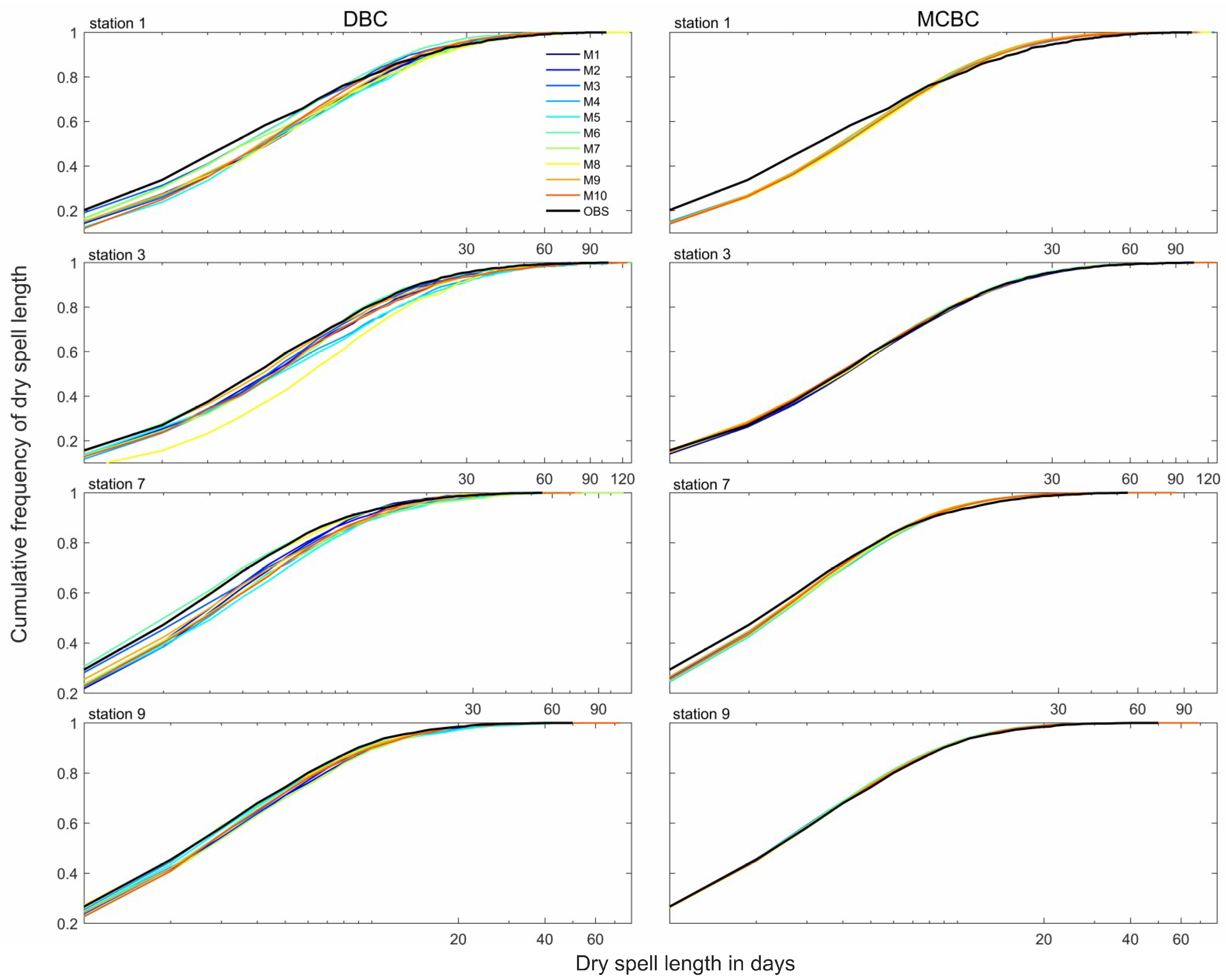
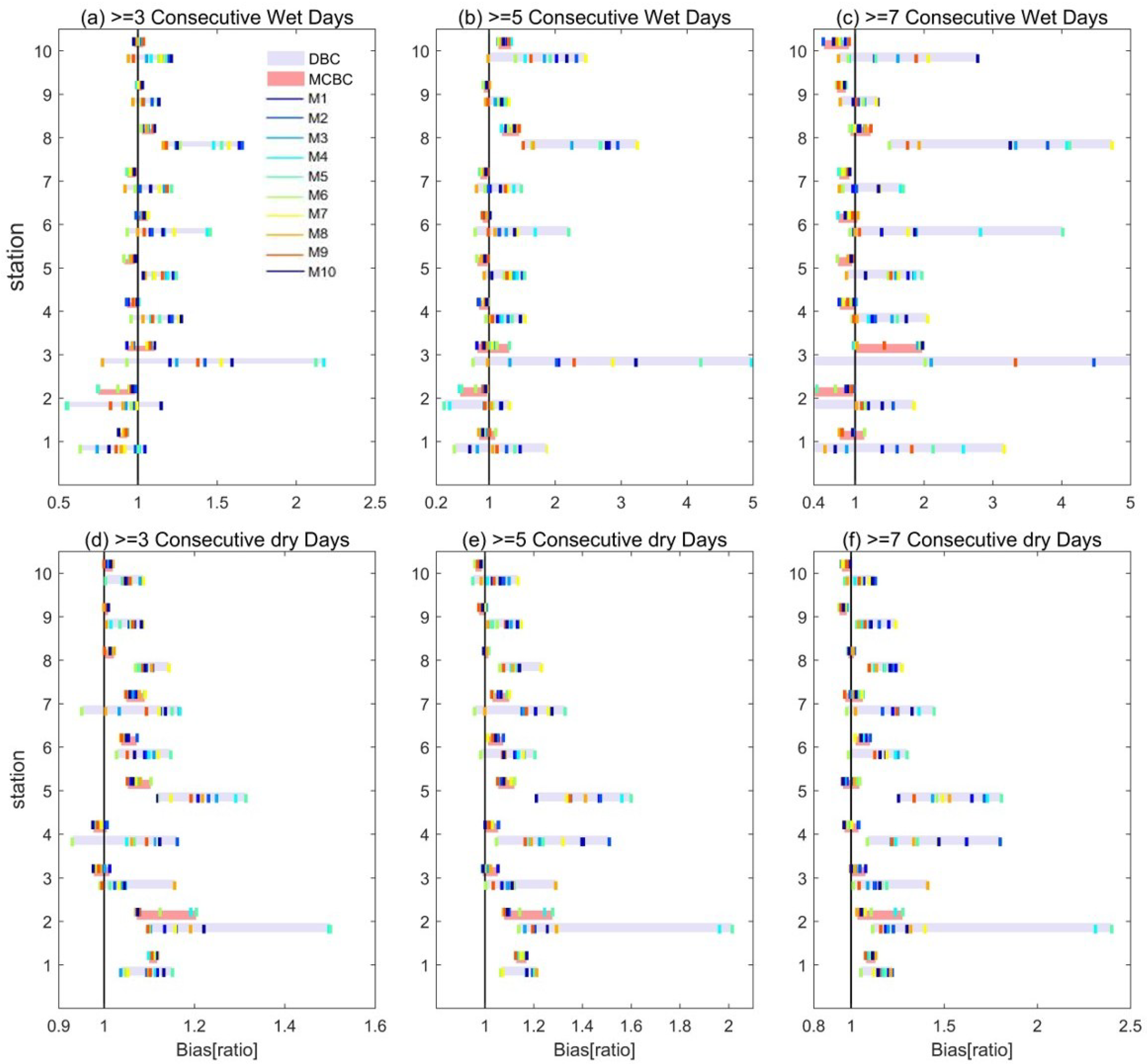
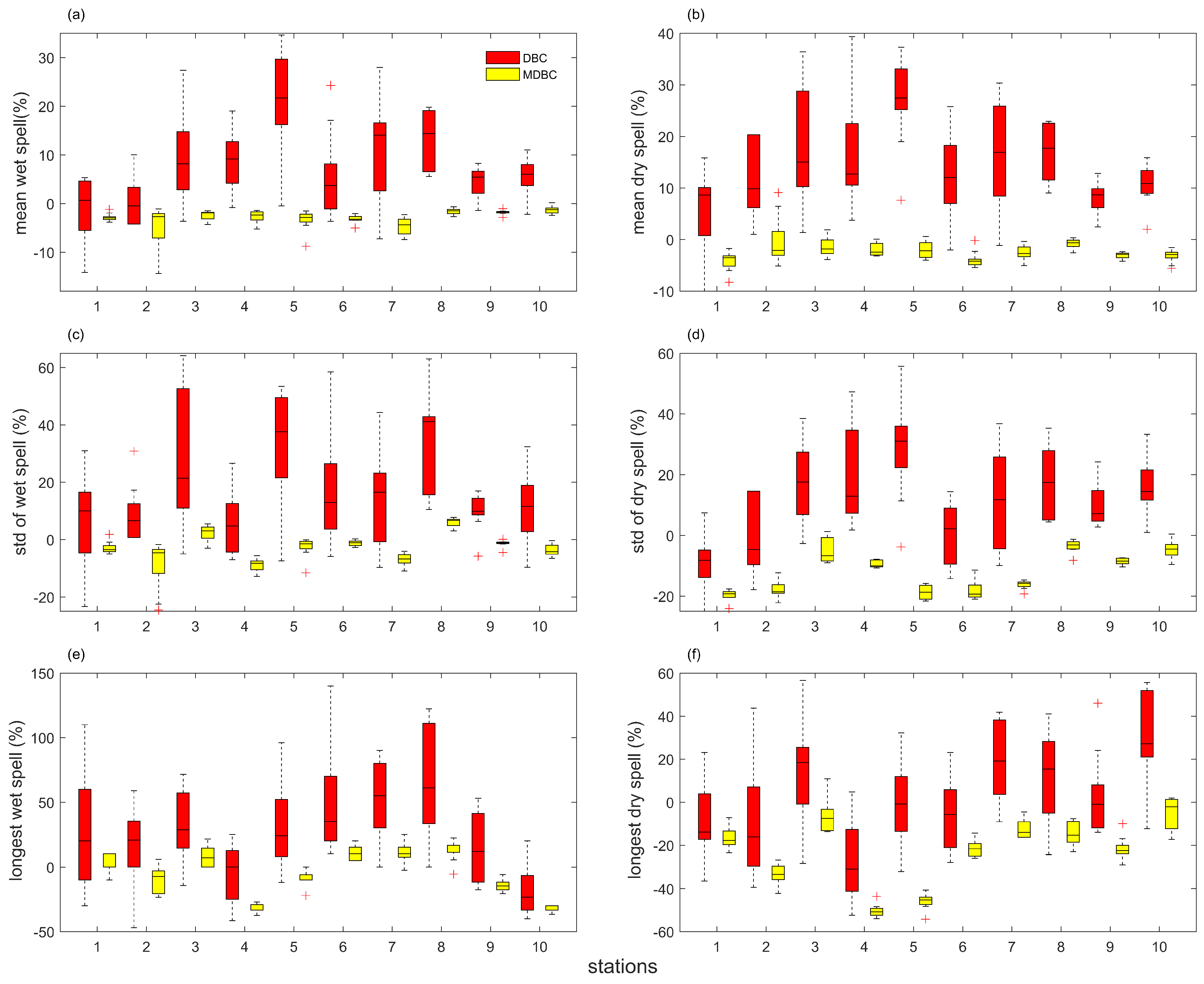
4.3. Performance of the MCBC Method

The performance of the MCBC method was first evaluated with respect to reproducing the cumulative frequencies of the observed wet- and dry-spell lengths. Figure 5 and Figure 6 present the cumulative frequencies of the wet- and dry-spell lengths generated by the DBC and MCBC methods (for one series), respectively. The cumulative frequencies of the observed wet- and dry-spell lengths were also used for comparison. Since similar results were obtained for all stations, only four stations from different climate zones were presented for illustrations. Generally, the DBC method underestimated the cumulative frequency of the wet- and dry-spells, except for the wet-spell of the first station (Figure 5). A significant uncertainty related to the choice of a GCM simulation was observed. However, the MCBC method largely reduced the biases of the cumulative frequency for the wet and dry spells. The uncertainty related to the GCMs was considerably corrected.
The K-S test showed that about 70% of the stations and GCM combinations (n = 10 stations × 10 GCMs) could not reject the null hypothesis for the cumulative frequencies of the wet- and dry-spells at the p = 0.05 significance level when using the proposed MCBC method. In other words, about 70% of cases were observed, and the bias-corrected cumulative frequencies may be from the same distribution. However, this value was only 20% when using the DBC method.
Consecutive wet days are an essential factor for high-impact flooding [33] and consecutive dry days for an extended period are one of the causes of droughts [48]. Accurately predicting the long wet- and dry-spell is vital for dealing with extreme hydrological events. Figure 7 shows the performances of the DBC (red bars) and MCBC (blue bars) methods in simulating the frequency of the spell lengths with more than or equal to 3, 5, and 7 consecutive dry days and wet days. The ratio of bias-corrected frequency to observed frequency was used as a metric to evaluate the performance of two bias correction methods. The closer the ratio was to 1, the more accurate the simulation. The results showed that the DBC method overestimated the frequencies of dry and wet spells for most stations. The result was expected, as the temporal structure was not specifically corrected by the DBC method. The MCBC method simulated the frequencies of dry and wet spells much better than the DBC method, indicated by the fact that the blue bars were shorter and closer to the baseline. Specifically, for the DBC method, the mean ratios across all stations with consecutive wet days being more than or equal to 3 days, 5 days, and 7 days ranged between 0.875 and 1.438, 0.938 and 2.471, 1.086 and 8.796, respectively. In contrast, the mean ratios for the MCBC method ranged between 0.909 and 1.074, 0.853 and 1.354, 0.772 and 1.434. Similar results were also observed for consecutive dry days.
Figure 8 shows the RE of the mean (Figure 8a,b), standard deviation (Figure 8c,d), and the longest length (Figure 8e,f) of wet- and dry-spells generated by the DBC and MCBC methods. The mean spell length simulated by the DBC method was considerably biased, with the median of REs ranging between −0.45% and 21.7% for the wet spell and between 8.62% and 27.44% for the dry spell. The MCBC method largely reduced the biases of the simulated mean spell length, with the median of REs ranging from −4.36% to −1.24% for the wet spell and ranging from −4.16% to −0.64% for the dry spell. More importantly, the uncertainty related to climate models was largely reduced. Similar results were also observed for the standard deviation of spell lengths (Figure 8c,d). The MCBC method also performed slightly better than the DBC method with respect to reproducing the longest wet and dry spell lengths, with the median of RE of 10-simulation medians ranging from −33.3% to 11.1% for the wet spell and ranging from −50.8% to −2.2% for the dry spell. For the DBC method, the median of RE ranged from −23.3% to 61.1% for the wet spell and from −31.0% to 27.2% for the dry spell. Although the benefits of the MCBC method are limited, the uncertainty related to climate model is reduced, with the interquartile ranges varying from 3.3% to 17.6% for the wet spell and ranging from 3.2% to 13.6% for the dry spell. In contrast, the interquartile ranges for the RE of the longest spell length simulated by the DBC method ranged from 26.6% to 77.8% for the wet spell and ranged from 20% to 36.6% for the dry spell.

5. Discussions and Conclusions

Accurately predicting the temporal sequence of precipitation occurrence at field or site-specific scales is critical in assessing climate change impacts on food security [42]. Daily soil water dynamics that are influenced mainly by daily precipitation sequences significantly affect crop growth and production, especially at the critical reproductive stages. More importantly, prolonged drought or wet spells can be detrimental to crop production. Thus, adequate simulation of wet- and dry-spell lengths is essential for adequately simulating the impacts of climate change on crop production and food security. Although bias correction methods, especially QM-based methods, can correct the precipitation amount simulated by climate models, the temporal sequence of precipitation occurrence is usually not explicitly considered. This study proposed a hybrid bias correction method to address the above problem. The MCBC method can be considered as a hybrid method combining QM bias correction and the stochastic Markov chain-based model. It not only has the advantage of the commonly used bias correction method in correcting the distributional attributes of precipitation amounts but it also takes advantage of the Markov chain in simulating the temporal sequence of precipitation occurrence. An evaluation of the proposed method showed that the temporal sequence of the precipitation occurrence was well corrected, and the proposed method consistently performed better than the traditional QM bias correction method. Specifically, the distribution of MCBC corrected wet- and dry-spell lengths fitted that of the observations very well, with the K-S test showing that more than 70% of the corrected series were likely from the same distribution of the observation at the p = 0.05 significance level. The MCBC method also reasonably reproduces the observed statistics of spell length, such as the frequency of spell length, mean, standard deviation, and the longest extreme spell length.
In addition, the Markov chain-based method used in this study is conceptually simple, easy to use, and requires less computation, because its parameters can be adjusted based on QM corrected results with a linear relationship of observed data. Even though the DBC model is applied as a baseline model in this study, the Markov chain-based model can be used with any other bias correction method. Moreover, this study uses the linear relationship between the observed mean monthly precipitation and the transition probabilities to adjust Markov chain parameters. Meanwhile, other methods can also be used, such as the analytical relationship between monthly mean precipitation, probability of rainfall occurrence, and daily mean precipitation as proposed by Wilks [49], and also the delta change method by Chen et al. [36]. Moreover, higher-order Markov chains may perform better than the first-order model in simulating precipitation sequence, especially for simulating dry spell length for long-durations over the dry regions [30,36,39,50]. However, as the order increases, the number of parameters also increases exponentially, and the parameter adjustment becomes more complicated [39]. By contrast, the first-order two-state Markov chain only has two parameters, and it is easy to operate and adequate in simulating wet and dry spells for various climates [30,39,49,51].
Since the main objective of this study was to propose a new bias correction method to deal with the biased temporal sequence of climate model simulated precipitation for field and site-specific food security studies, the inter-variable correlations and the inter-site correlation of precipitation time series were not considered. While the correlation between precipitation and temperature, as well as solar radiation, is an essential input to crop and hydrological models, for some other studies, such as hydrological impact studies, the precipitation time series over multiple sites within a watershed may be needed to study the spatial variability of climate change impacts. However, the inter-variable and inter-site correlation can be easily induced using a post-processing method, such as the distribution-free shuffle approach [52,53,54] and the copula-based method [55,56]. The post-processing method can be an avenue for future studies.

Author Contributions

Conceptualization, J.C. and H.L.; methodology, X.-C.Z.; software, Y.H.; validation, H.L.; writing—original draft preparation, H.L.; writing—review and editing, C.-Y.X.; funding acquisition, J.C. All authors have read and agreed to the published version of the manuscript.

Funding

This research was funded by the National Key Research and Development Program of China, grant number 2017YFA0603704, by the National Natural Science Foundation of China, grant number 51779176 and 51539009, and the Overseas Expertise Introduction Project for Discipline Innovation (111 Project) funded by the Ministry of Education and State Administration of Foreign Experts Affairs P.R. China, grant number B18037.

Acknowledgments

This work was partially supported by the National Key Research and Development Program of China (No. 2017YFA0603704), the National Natural Science Foundation of China (Grant No. 51779176, 51539009), and the Overseas Expertise Introduction Project for Discipline Innovation (111 Project) funded by the Ministry of Education and State Administration of Foreign Experts Affairs P.R. China (Grant No. B18037). The authors would like to acknowledge the China Meteorological Data Sharing Service System for providing datasets for the ten stations.

Conflicts of Interest

The authors declare no conflict of interest.

References

  1. Chen, J.; Brissette, F.P.; Poulin, A.; Leconte, R. Overall uncertainty study of the hydrological impacts of climate change for a Canadian watershed. Water Resour. Res. 2011, 47. [Google Scholar] [CrossRef]
  2. Jeong, H.; Bhattarai, R.; Hwang, S. How climate scenarios alter future predictions of field-scale water and nitrogen dynamics and crop yields. J. Environ. Manag. 2019, 252, 109623. [Google Scholar] [CrossRef] [PubMed]
  3. Ramirez-Villegas, J.; Challinor, A.J.; Thornton, P.K.; Jarvis, A. Implications of regional improvement in global climate models for agricultural impact research. Environ. Res. Lett. 2013, 8, 024018. [Google Scholar] [CrossRef]
  4. Wang, G. Agricultural drought in a future climate: Results from 15 global climate models participating in the IPCC 4th assessment. Clim. Dyn. 2005, 25, 739–753. [Google Scholar] [CrossRef]
  5. Chen, J.; Brissette, F.P.; Leconte, R. Uncertainty of downscaling method in quantifying the impact of climate change on hydrology. J. Hydrol. 2011, 401, 190–202. [Google Scholar] [CrossRef]
  6. Chen, J.; Chen, H.; Guo, S. Multi-site precipitation downscaling using a stochastic weather generator. Clim. Dyn. 2017, 50, 1975–1992. [Google Scholar] [CrossRef]
  7. Martins, M.A.; Tomasella, J.; Dias, C.G. Maize yield under a changing climate in the Brazilian Northeast: Impacts and adaptation. Agric. Water Manag. 2019, 216, 339–350. [Google Scholar] [CrossRef]
  8. Jakob Themeßl, M.; Gobiet, A.; Leuprecht, A. Empirical-statistical downscaling and error correction of daily precipitation from regional climate models. Int. J. Climatol. 2011, 31, 1530–1544. [Google Scholar] [CrossRef]
  9. Troin, M.; Velázquez, J.A.; Caya, D.; Brissette, F. Comparing statistical post-processing of regional and global climate scenarios for hydrological impacts assessment: A case study of two Canadian catchments. J. Hydrol. 2015, 520, 268–288. [Google Scholar] [CrossRef]
  10. Chen, J.; Brissette, F.P.; Chaumont, D.; Braun, M. Performance and uncertainty evaluation of empirical downscaling methods in quantifying the climate change impacts on hydrology over two North American river basins. J. Hydrol. 2013, 479, 200–214. [Google Scholar] [CrossRef]
  11. Ines, A.V.; Hansen, J.W. Bias correction of daily GCM rainfall for crop simulation studies. Agric. For. Meteorol. 2006, 138, 44–53. [Google Scholar] [CrossRef] [Green Version]
  12. Maraun, D.; Shepherd, T.G.; Widmann, M.; Zappa, G.; Walton, D.; Gutiérrez, J.M.; Mearns, L.O. Towards process-informed bias correction of climate change simulations. Nat. Clim. Chang. 2017, 7, 764–773. [Google Scholar] [CrossRef] [Green Version]
  13. Manzanas, R.; Gutiérrez, J.M.; Bhend, J.; Hemri, S.; Doblas-Reyes, F.J.; Torralba, V.; Penabad, E.; Brookshaw, A. Bias adjustment and ensemble recalibration methods for seasonal forecasting: A comprehensive intercomparison using the C3S dataset. Clim. Dyn. 2019, 53, 1287–1305. [Google Scholar] [CrossRef]
  14. Caya, D.; Laprise, R. A semi-implicit semi-lagrangian regional climate model: The canadian rcm. Mon. Weather Rev. 1999, 127, 341–362. [Google Scholar] [CrossRef]
  15. Teutschbein, C.; Seibert, J. Regional Climate Models for Hydrological Impact Studies at the Catchment Scale: A Review of Recent Modeling Strategies. Geogr. Compass 2010, 4, 834–860. [Google Scholar] [CrossRef] [Green Version]
  16. Zhang, X.C.; Chen, J.; Garbrecht, J.D.; Brissette, F.P. Evaluation of a weather generator-based method for statistically downscaling non-stationary climate scenarios for impact at point scale. Trans. ASAE 2012, 55, 1745–1756. [Google Scholar] [CrossRef]
  17. Fowler, H.J.; Ekström, M.; Blenkinsop, S.; Smith, A.P. Estimating change in extreme European precipitation using a multimodel ensemble. J. Geophys. Res. 2007, 112. [Google Scholar] [CrossRef] [Green Version]
  18. Murphy, J. An Evaluation of Statistical and Dynamical Techniques for Downscaling Local Climate. J. Clim. 1999, 12, 2256–2284. [Google Scholar] [CrossRef]
  19. Zhang, X.C. Verifying a temporal disaggregation method for generating daily precipitation of potentially non-stationary climate change for site-specific impact assessment. Int. J. Climatol. 2013, 33, 326–342. [Google Scholar] [CrossRef]
  20. Cannon, A.J.; Sobie, S.R.; Murdock, T.Q. Bias Correction of GCM Precipitation by Quantile Mapping: How Well Do Methods Preserve Changes in Quantiles and Extremes? J. Clim. 2015, 28, 6938–6959. [Google Scholar] [CrossRef]
  21. Chen, J.; Brissette, F.P.; Chaumont, D.; Braun, M. Finding appropriate bias correction methods in downscaling precipitation for hydrologic impact studies over North America. Water Resour. Res. 2013, 49, 4187–4205. [Google Scholar] [CrossRef]
  22. Teutschbein, C.; Seibert, J. Bias correction of regional climate model simulations for hydrological climate-change impact studies: Review and evaluation of different methods. J. Hydrol. 2012, 456, 12–29. [Google Scholar] [CrossRef]
  23. Hnilica, J.; Hanel, M.; Puš, V. Multisite bias correction of precipitation data from regional climate models. Int. J. Climatol. 2017, 37, 2934–2946. [Google Scholar] [CrossRef]
  24. Rosenberg, E.A.; Keys, P.W.; Booth, D.B.; Hartley, D.; Burkey, J.; Steinemann, A.C.; Lettenmaier, D.P. Precipitation extremes and the impacts of climate change on stormwater infrastructure in Washington State. Clim. Chang. 2010, 102, 319–349. [Google Scholar] [CrossRef] [Green Version]
  25. Schoof, J.T.; Shin, D.W.; Cocke, S.; LaRow, T.E.; Lim, Y.K.; O’Brien, J.J. Dynamically and statistically downscaled seasonal temperature and precipitation hindcast ensembles for the southeastern USA. Int. J. Climatol. 2009, 29, 243–257. [Google Scholar] [CrossRef] [Green Version]
  26. Roosmalen, L.V.; Christensen, J.H.; Butts, M.B.; Jensen, K.H.; Refsgaard, J.C. An intercomparison of regional climate model data for hydrological impact studies in Denmark. J. Hydrol. 2010, 380, 406–419. [Google Scholar] [CrossRef]
  27. Schmidli, J.; Frei, C.; Vidale, P.L. Downscaling from GCM precipitation: A benchmark for dynamical and statistical downscaling methods. Int. J. Climatol. 2006, 26, 679–689. [Google Scholar] [CrossRef]
  28. Themeßl, M.J.; Gobiet, A.; Heinrich, G. Empirical-statistical downscaling and error correction of regional climate models and its impact on the climate change signal. Clim. Chang. 2012, 112, 449–468. [Google Scholar] [CrossRef]
  29. Shen, M.; Chen, J.; Zhuan, M.; Chen, H.; Xu, C.-Y.; Xiong, L. Estimating uncertainty and its temporal variation related to global climate models in quantifying climate change impacts on hydrology. J. Hydrol. 2018, 556, 10–24. [Google Scholar] [CrossRef]
  30. Chen, J.; Zhang, X.J.; Brissette, F.P. Assessing scale effects for statistically downscaling precipitation with GPCC model. Int. J. Climatol. 2014, 34, 708–727. [Google Scholar] [CrossRef]
  31. Ines, A.V.; Hansen, J.W.; Robertson, A.W. Enhancing the utility of daily GCM rainfall for crop yield prediction. Int. J. Climatol. 2011, 31, 2168–2182. [Google Scholar] [CrossRef] [Green Version]
  32. Maraun, D.; Wetterhall, F.; Ireson, A.M.; Chandler, R.E.; Kendon, E.J.; Widmann, M.; Brienen, S.; Rust, H.W.; Sauter, T.; Themeßl, M.; et al. Precipitation downscaling under climate change: Recent developments to bridge the gap between dynamical models and the end user. Rev. Geophys. 2010, 48. [Google Scholar] [CrossRef]
  33. Rajczak, J.; Kotlarski, S.; Schär, C. Does Quantile Mapping of Simulated Precipitation Correct for Biases in Transition Probabilities and Spell Lengths? J. Clim. 2016, 29, 1605–1615. [Google Scholar] [CrossRef]
  34. Chen, J.; Brissette, F.P. Comparison of five stochastic weather generators in simulating daily precipitation and temperature for the Loess Plateau of China. Int. J. Climatol. 2014, 34, 3089–3105. [Google Scholar] [CrossRef]
  35. Chen, J.; Brissette, F.P.; Leconte, R. A daily stochastic weather generator for preserving low-frequency of climate variability. J. Hydrol. 2010, 388, 480–490. [Google Scholar] [CrossRef]
  36. Chen, J.; Brissette, F.P.; Leconte, R. Downscaling of weather generator parameters to quantify hydrological impacts of climate change. Clim. Res. 2012, 51, 185–200. [Google Scholar] [CrossRef] [Green Version]
  37. Moon, S.-E.; Ryoo, S.-B.; Kwon, J.-G. A Markov chain model for daily precipitation occurrence in South Korea. Int. J. Climatol. 1994, 14, 1009–1016. [Google Scholar] [CrossRef]
  38. Wilks, D.S. Multisite generalization of a daily stochastic precipitation generation model. J. Hydrol. 1998, 210, 178–191. [Google Scholar] [CrossRef]
  39. Wilks, D.S. Interannual variability and extreme-value characteristics of several stochastic daily precipitation models. Agric. For. Meteorol. 1999, 93, 153–169. [Google Scholar] [CrossRef]
  40. Wilks, D.S. Multisite downscaling of daily precipitation with a stochastic weather generator. Clim. Res. 1999, 11, 125–136. [Google Scholar] [CrossRef] [Green Version]
  41. Wilks, D.S.; Wilby, R.L. The weather generation game: A review of stochastic weather models. Prog. Phys. Geogr. 1999, 23, 329–357. [Google Scholar] [CrossRef]
  42. Apipattanavis, S.; Podestá, G.; Rajagopalan, B.; Katz, R.W. A semiparametric multivariate and multisite weather generator. Water Resour. Res. 2007, 43, 1973–1989. [Google Scholar] [CrossRef]
  43. Gu, L.; Chen, J.; Xu, C.-Y.; Wang, H.-M.; Zhang, L. Synthetic Impacts of Internal Climate Variability and Anthropogenic Change on Future Meteorological Droughts over China. Water 2018, 10, 1702. [Google Scholar] [CrossRef] [Green Version]
  44. Zhuan, M.-J.; Chen, J.; Shen, M.-X.; Xu, C.-Y.; Chen, H.; Xiong, L.-H. Timing of human-induced climate change emergence from internal climate variability for hydrological impact studies. Hydrol. Res. 2018, 49, 421–437. [Google Scholar] [CrossRef]
  45. Mpelasoka, F.S.; Chiew, F.H. Influence of Rainfall Scenario Construction Methods on Runoff Projections. J. Hydrometeorol. 2009, 10, 1168–1183. [Google Scholar] [CrossRef]
  46. Gabriel, K.R.; Neumann, J. A markov chain model for daily rainfall occurrence at tel aviv. Q. J. R. Meteorol. Soc. 2010, 88, 90–95. [Google Scholar] [CrossRef]
  47. Li, Z.; Brissette, F.; Chen, J. Assessing the applicability of six precipitation probability distribution models on the Loess Plateau of China. Int. J. Climatol. 2014, 34, 462–471. [Google Scholar] [CrossRef]
  48. Heim, R.R. A Review of Twentieth-Century Drought Indices Used in the United States. Bull. Am. Meteorol. Soc. 2002, 83, 1149–1166. [Google Scholar] [CrossRef] [Green Version]
  49. Wilks, D.S. Adapting stochastic weather generation algorithms for climate change studies. Clim. Chang. 1992, 22, 67–84. [Google Scholar] [CrossRef]
  50. Schoof, J.T.; Pryor, S.C. On the Proper Order of Markov Chain Model for Daily Precipitation Occurrence in the Contiguous United States. J. Appl. Meteorol. Climatolo. 2008, 47, 2477–2486. [Google Scholar] [CrossRef]
  51. Zhang, X.C.; Garbrecht, J.D. Evaluation of CLIGEN precipitation parameters and their implication on WEPP runoff and erosion prediction. Tran. ASAE 2003, 46, 311. [Google Scholar]
  52. Iman, R.L.; Conover, W.J. A distribution-free approach to inducing rank correlation among input variables. Commun. Stat. Simul. Comput. 2007, 11, 311–334. [Google Scholar] [CrossRef]
  53. Li, Z. A new framework for multi-site weather generator: A two-stage model combining a parametric method with a distribution-free shuffle procedure. Clim. Dyn. 2013, 43, 657–669. [Google Scholar] [CrossRef]
  54. Zhang, X.C. Generating correlative storm variables for CLIGEN using a distribution-free approach. Trans. ASAE 2005, 48, 567–575. [Google Scholar] [CrossRef]
  55. Li, X.; Babovic, V. Multi-site multivariate downscaling of global climate model outputs: An integrated framework combining quantile mapping, stochastic weather generator and Empirical Copula approaches. Clim. Dyn. 2019, 52, 5775–5799. [Google Scholar] [CrossRef]
  56. Li, X.; Babovic, V. A new scheme for multivariate, multisite weather generator with inter-variable, inter-site dependence and inter-annual variability based on empirical copula approach. Clim. Dyn. 2019, 52, 2247–2267. [Google Scholar] [CrossRef]
Figure 1. The location of the ten stations in China.
Atmosphere 11 00109 g001
Figure 2. Relative errors (REs) of the mean monthly precipitation for all 12 calendar months at all ten stations. The red boxplots present the ensemble of the raw GCM simulations, and the yellow boxplots present the DBC corrected results.
Atmosphere 11 00109 g002
Figure 3. Relationships between the conditional precipitation occurrence probabilities of wet-following-wet (P11) and wet-following-dry (P01) and mean monthly precipitation amounts in January for all stations.
Atmosphere 11 00109 g003
Figure 4. Relationships between the conditional precipitation occurrence probabilities of wet-following-wet (P11) and wet-following-dry (P01) and mean monthly precipitation amounts in July for all stations.
Atmosphere 11 00109 g004
Figure 5. The corrected and observed cumulative frequencies of wet spell lengths for stations 1, 3, 7, and 9. The black line represents the cumulative frequencies of observation. M1-M10 represents 10 GCMs corresponding to the order in Table 2. The X-axis is on a logarithmic scale.
Atmosphere 11 00109 g005
Figure 6. The corrected and observed cumulative frequencies of dry spell lengths for stations 1, 3, 7, and 9. The black line represents the cumulative frequencies of observation. M1-M10 represents 10 GCMs corresponding to the order in Table 2. The X-axis is on a logarithmic scale.
Atmosphere 11 00109 g006
Figure 7. The bias on the frequency of spell lengths with (a) ≥3, (b) ≥5, and (c) ≥consecutive wet days. The bias on the frequency of spell lengths with (d) ≥3, (e) ≥5, and (f) ≥7 consecutive dry days. The bias is represented as the ratio of the simulated series to observations. The range of the color represents the ensemble of 10 simulations. M1-M10 represents 10 GCMs corresponding to the order in Table 2.
Atmosphere 11 00109 g007
Figure 8. RE statistics of the wet- and dry spell lengths generated by the two bias correction methods for all ten stations. (a) Mean wet spell, (b) mean dry spell, (c) standard deviation of wet spell, (d) standard deviation of dry spell, (e) longest wet spell, and (f) longest dry spell.
Atmosphere 11 00109 g008
Table 1. Name, location, mean annual precipitation, and wet day frequency of the ten stations.
StationNameLatitude
(°N)
Longitude
(°E)
Elevation
(m)
Mean Annual Precipitation (mm)Wet Day Frequency
1Wuqia39.7275.2521761850.18
2Bayinbuluke43.0384.1524582770.32
3Alashanzuoqi38.83105.6715612090.15
4Langzhong31.58105.9738310280.37
5Fengshan24.55107.0348715260.44
6Anyang36.05114.40635620.20
7Xianyou25.37118.7080015650.39
8Dalian38.90121.63926230.21
9Sunwu49.43127.352105400.32
10Xinerbahuyouqi48.67116.825542410.18
Table 2. Name, source and resolution of the ten global climate models.
No.Model NameModelling CentreSourceSpatial Resolution
(Longitude × Latitude)
1ACCESS-1.0CRIRO-BOMCommonwealth Scientific and Industrial Research Organization (CSIRO) and Bureau of Meteorology (BOM), Australia1.875° × 1.25°
2CESM1-CAM5NSF-DOE-NCARNational Science Foundation, Department of Energy National Center for Atmospheric Research1.25° × 0.94°
3CMCC-CMCMCCCentro Euro-Mediterraneo per I Cambiamenti Climatici0.75° × 0.75°
4CSIRO-Mk3-6.0CSIRO-QCCCECommonwealth Scientific and Industrial Research Organization in collaboration with Queensland Climate Change Centre of Excellence1.90° × 1.90°
5FGOALS-G2LASG-CESSLASG, Institute of Atmospheric Physics, Chinese Academy of Sciences and CESS, Tsinghua University2.81° × 3.00°
6GFDL-ESM2GNOAA GFDLNOAA Geophysical Fluid Dynamics Laboratory2.50° × 2.0°
7GFDL-ESM2M
8MIROC5MIPOCAtmosphere and Ocean Research Institute (The University of Tokyo), National Institute for Environmental Studies, and Japan Agency for Marine-Earth Science and Technology1.40° × 1.40°
9MRI-CGCM3MRIMeteorological Research Institute1.10° × 1.10°
10MRI-ESM11.13° × 1.13°

