Article

Low Polluting Building Materials and Ventilation for Good Air Quality in Residential Buildings: A Cost–Benefit Study

Institute for Renewable Energy, Eurac Research, 39100 Bolzano, Italy
*
Author to whom correspondence should be addressed.
Atmosphere 2020, 11(1), 102; https://doi.org/10.3390/atmos11010102
Submission received: 11 November 2019 / Revised: 9 January 2020 / Accepted: 10 January 2020 / Published: 15 January 2020
(This article belongs to the Special Issue Green Buildings and Indoor Air Quality)

Abstract

:
Nowadays, people spend an average of 87% of their time inside buildings, and about 69% at home. Hence, it is essential to ensure the highest possible level of indoor air quality (IAQ). Providing that the quality of the outdoor air is acceptable, the IAQ level is improved by increasing the ventilation rates. However, this means that a larger volume of air must be cooled down or warmed up to ensure the same level of thermal comfort. The aim of this study was to conduct a cost–benefit analysis of the IAQ in residential buildings. A case-study building was defined, and three sets of materials with different pollution emission levels were chosen: High, low, and very low. For each option, the ventilation rates required to have the same IAQ level were calculated, and the consequent energy consumption and costs were estimated by means of dynamic thermal simulation. The results show the range of the initial capital cost that could be compensated for by lower running costs, and the effect of each energy and economic input assumption on the appraisal of the affordable capital cost. In the discussion, insights into the IAQ co-benefits are also given.

1. Introduction

Nowadays, people spend an average of 87% of their time inside buildings, and about 69% at home [1]. Hence, it is essential to ensure the highest possible level of indoor air quality (IAQ), which is affected by indoor and outdoor pollution sources. Providing that the quality of outdoor air is acceptable or that filters are used, the IAQ level is usually improved by increasing the ventilation rates. However, depending on the season, this means that a larger volume of air must be cooled down or warmed up to ensure the same level of thermal comfort, leading to higher energy consumption and associated costs. Energy consumption in residential buildings already accounts for more than 25% of the entire energy consumption in the EU [2], and this figure is likely to increase. Therefore, it is important to identify means to revise this upward trend without jeopardizing the indoor environmental quality (IEQ).
IAQ is one of the four IEQ components (the others are thermal, visual, and acoustic comfort) and it refers to the nature of air that affects the health and well-being of occupants. ASHRAE Standard 62.1–2016 [3] defines acceptable IAQ as the “air in which there are no known contaminants at harmful concentrations as determined by cognizant authorities and with which a substantial majority (80% or more) of the people exposed do not express dissatisfaction”.
The World Health Organization (WHO) estimated that 23% of global deaths are linked to an unhealthy living or working environment [4]. The health effects of indoor air pollutants might emerge immediately after exposure as well as several years later. In addition to the duration of exposure, it is essential to consider the corresponding exposure limit value (ELV) in order to determine the harmfulness of a pollutant in a certain environment [5]. In other words, the pollutant level and exposure time have to be considered together to evaluate the level of risk.
Air is a complex mixture typically composed of more than 200 to 300 pollutants [6]. The European Respiratory Society (ERS) has identified the most important pollutants of indoor air, namely carbon monoxide (CO), carbon dioxide (CO2), nitrogen dioxide or trioxide (NO2–NO3), polycyclic aromatic hydrocarbons (PHAs), particulate matter (PM2.5, PM10, etc.), volatile organic compounds (VOCs), allergens, formaldehyde (H−CHO), radon, biological contaminants, and ozone (O3) [7].
All these compounds are usually present in indoor air, with different concentrations depending on the emission rate of the relative sources and the ventilation rate of the room. Thus, an analysis of the presence of specific sources is essential to assess the risk of exposure to certain contaminants, and to suggest solutions to decrease the contaminant concentration below acceptable thresholds.
Most indoor pollutants derive from anthropogenic sources [7] that can be divided into indoor and outdoor ones. The former category comprises building materials (construction materials, furniture, paintings, ventilation ducts, etc.), cleaning products, heating and cooking appliances, people, and clothes while the most diffused outdoor sources are related to combustion processes in industrial and domestic plants and vehicles.
Focusing on indoor pollution sources and substances and residential buildings, two key pollutants are formaldehyde and CO2. Formaldehyde is a volatile organic compound (VOC) that has been discussed for decades as a typical indoor pollutant [8], which derives from construction materials or furniture, and is very harmful as it is carcinogenic. The analysis of a collection of formaldehyde measurement data from residential buildings in different countries shows concentrations often close to the short-term guideline value of 100 µg/m3 proposed by the WHO Guideline for IAQ [9]. CO2 is generated during the respiration processes of living aerobic organisms. CO2 is considerably less harmful than formaldehyde, but it is typically used to control ventilation as a proxy for the other contaminants, or as an indicator of the occupancy of the indoor environment.
Low-cost furniture (and often low-cost building materials, in general) is a common source of formaldehyde in domestic buildings, and the spread of this more affordable type of furniture is constantly increasing. To solve this problem, two possible routes are ventilating more or purchasing less pollutant products. The former option means higher running costs for energy, the latter a higher capital cost. However, to date, too little is known about the economic comparability of these two routes. Indeed, previous studies on IAQ, ventilation, and economics [10,11] focused on other approaches and metrics, such as disability-adjusted life years (DALYs), that provide a method of monetizing contaminant exposure.
The aim of this study was therefore to conduct a cost–benefit analysis of the IAQ in residential buildings. A case-study building was defined, and three sets of materials with different pollution emission levels were chosen: High, low, and very low. For each option, the ventilation rates required to have an acceptable IAQ level were calculated, and the consequent energy consumption (and associated costs) were estimated by means of dynamic thermal simulation in EnergyPlus. In general, it was found that less polluting elements are more expensive but less ventilation, and hence costs, are then needed.

2. Methodology

2.1. Analytical Modelling of the Contaminants and Ventilation Rates

2.1.1. Contaminants Emission Rates

In this study, the generation and removal of two air pollutants were considered, namely formaldehyde (as a pollutant related to building materials) and carbon dioxide produced by human respiration. For formaldehyde, three emission classes were defined: High-emitting (HE), low-emitting (LE), and very low-emitting (VLE) building. These three building typologies are characterized by the presence of construction materials with different formaldehyde emission levels. For the purpose of the study, formaldehyde might come from both furniture and interior finishing, such wall and floor treatments.
The determination of the formaldehyde emission rate was based on the Finnish M1 volunteer emission labeling system [12]. The choice of this classification system was based on the fact that this is the only material labeling protocol that classifies the tested products according to an area-specific emission rate (i.e., emission per unit of surface). Indeed, the other common protocols classify materials’ emissions according to the pollutant’s concentration in air after a certain period of permanence in a test chamber under well-defined conditions, and this does not enable the calculation of emission rates to be implemented in a dynamic thermal model.
In particular, the M1 labeling system defines three emission classes called M1, M2, and M3, where M1 corresponds to the best quality emission class. To be certified in a certain class, a material must fulfill several criteria in terms of emissions related to different pollutants after four weeks: Total volatile organic compounds (TVOCs), single VOCs, formaldehyde, ammonia, and compounds belonging to carcinogen categories 1A or 1B.
In this study, the guideline values for the formaldehyde protocol were used to set up the emission rates for low- and very low-emitting materials. On the other hand, for high-emitting materials, the area-specific emission rate was selected according to an evaluation of different wood-based construction materials available within the ContamLink database [13]. An average emission rate for a medium density fiberboard was chosen [14]. Table 1 shows the selected area-specific emission rates for the three different building typologies. For each room, a loading factor of 0.3 m2/m3 corresponding to the floor area was defined. Thus, the emission rates were multiplied by the area of the floor of each thermal zone, resulting in a room-specific emission rate. These emission rates were assumed to be constant over time, and the implications of this assumption are discussed later in the paper.
In addition to the formaldehyde emission rates, the CO2 generated by the occupants was calculated. The generation of carbon dioxide mainly depends on the activity level of the person, assumed to be equal to 1 met (i.e., seated quiet person [15]) for the occupants of the living room and 0.7 met (i.e., sleeping person) for people occupying the bedroom. The rate of CO2 generation, GCO2, of l/s per person was calculated according to the equation provided by the ASHRAE Handbook of Fundamentals [16] (Equation (1)). The CO2 generation rate per person was then multiplied by the actual number of people occupying each room according to the occupancy schedule implemented in the energy model:
G C O 2 = G O 2 · R Q = 0.00276 · A D · M ( 0.23 · R Q + 0.77 ) · R Q ,
where G C O 2 is the CO2 generation rate per person (L/s); A D is the Dubois area (m2); R Q is the respiratory quotient (–); and M is the metabolic rate (met).
The CO2 generation rates of the standard method were compared with those resulting from a new approach based on concepts from the fields of human metabolism and exercise physiology and also considering the variability that may occur based on body mass [17]. Unlike the ASHRAE method, the new approach considers the dependency on the age and sex and thus the body mass and the basal metabolic rate (BMR).
However, in the present study, considering the variability in CO2 generation rates among different building occupants would also not have made a substantial impact on the results. Indeed, as a first step, a standard adult occupant with a Dubois area of 1.8 m2 was considered and the ASHRAE method applied. The resulting CO2 generation rate of 0.0043 L/s in the case of a metabolic rate of 1 met is comparable with the one resulting from the new approach, in the case of a male between 21 and 30 years and an air temperature correction to 293 K, which amounts to 0.0042 L/s. More substantial variations would occur only considering scenarios (e.g., very low temperature conditions, such as 0 °C, or occupants with different basal metabolic rates) that are out of the scope of the present study. Hence, the standard ASHRAE models were used in this study.

2.1.2. Ventilation Rates

In order to guarantee good indoor air quality, the concentration of pollutants must be kept below a certain threshold value. Different guideline values for long- and short-term exposure are available in the standards. In the case of the formaldehyde, the most commonly used exposure limit value (ELV) refers to a short-term 30-min exposure to an amount of 0.1 mg/m3. This guideline value is given by the WHO Guideline for IAQ [9] and adopted in many national legislations. Instead, for long-term exposure, there is no clear evidence for a threshold value. Thus, for this study, the guideline value for formaldehyde concentration suggested by the standard CEN/TR 16798-2:2019 [18] for very low-emitting materials was used. Hence, the formaldehyde guideline value for long-term exposure was fixed at 0.03 mg/m3. For CO2, instead, the indoor design concentration was selected according to category 2 (i.e., normal level of expectation, which is the suggested level for residential buildings) of the standard EN 16798-1:2019 [17] and is equal to 1200 ppm.
According to the methodology suggested by the EN16798-2: 2019 standard, the design ventilation rates were calculated as the ventilation rates needed to dilute CO2 and formaldehyde below the guideline levels mentioned above, and making the following assumptions:
  • Well-mixed internal air;
  • Constant external CO2 concentration (400 ppm); and
  • Zero external formaldehyde concentration.
Thus, the ventilation rate was calculated by solving the mass balance for each contaminant, as described in Equations (2) and (3), and taking the highest ventilation rate of the two (CO2 and HCHO-based value):
V d C d t = G + Q C o u t Q C ,
C = C t 1 e t Q / V + ( C o u t + G Q ) ( 1 e t Q / V ) ,
where V is the air volume (m3); C is the inside concentration of contaminant i at time t (µg/m3); C t 1 is the inside concentration of contaminant i at a previous time-step (µg/m3); C o u t is the constant outside concentration of contaminant i (µg/m3); t is the time (s); and Q is the ventilation rate (m3/s).
Due to these assumptions, the level of accuracy of the model is not suitable for the evaluation of smart ventilation systems based on the exposure level evaluation rather than on single contaminants’ concentrations. However, it is appropriate for comparing different levels of ventilation in terms of energy and economic costs.

2.2. Dynamic Thermal Modelling

The case-study building represents the typical archetype of new single-family houses in Alto Adige/South Tyrol (northern Italy). To some extent, this building is also representative of the recent residential buildings in neighboring alpine regions, such as Tyrol (Austria). The building was chosen by combining the two sources, namely the output of an analysis of the building stock in a valley in South Tyrol, conducted by means of a database provided by the Austrian and Italian TABULA project [19], and the guidelines and database of the local energy certification agency called Agenzia per l’Energia Alto Adige-CasaClima.
The case-study building was modelled and simulated with EnergyPlus 8.7.0 (US Department of Energy’s (DOE), USA). Each simulation was performed on a timestep of 15 min over a whole reference year. The weather file chosen to run the simulations was generated by Meteonorm using extreme hourly values over a 10-year weather time series for the city of Bolzano, which is the provincial capital of South Tyrol.

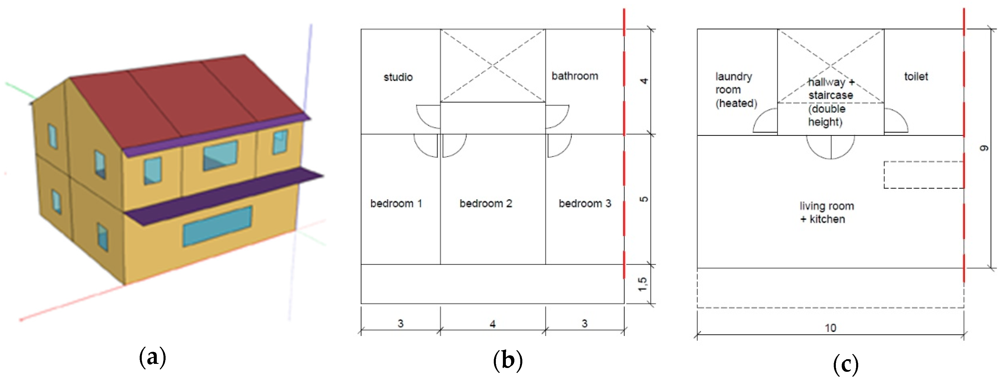
2.2.1. Geometry and Construction Type

The model consisted of nine thermal zones, one for each room (Figure 1) and one for the staircase. The living area is located on the ground floor while the sleeping area on the first floor. The building has a net floor area of 124 m2 and a floor-to-ceiling height of 2.7 m. The west façade was assumed to be adjacent to another similar building; thus, it was considered as adiabatic.
The characteristics of the construction elements are summarized in Table 2. The thermal performance of the construction elements is compliant with the current local building energy performance code and regulations.

2.2.2. Internal Gains

Schedules for occupancy, lighting, and electric equipment reported in the 2014 Building America House Simulation Protocol [20] were applied since it considers disaggregated schedules for living room and bedrooms, as well as for weekdays and weekends.
The total number of occupants in the building was assumed as being equal to four, and the occupancy profile was calculated considering their presence in the living area (ground floor) and sleeping area (first floor) over weekdays and weekends. The total heat gains related to occupants were calculated according to typical metabolic heat generation for domestic activities [16], namely 126 W/person for occupants in the living area, and 72 W/person for occupants in the sleeping area.
Lighting and electric equipment gains were scheduled according to the occupancy schedule. The electric lights in the living room were also dimmed according to the daylighting level. Two reference points were placed in the living room at 0.8 m above the floor. Daylighting illuminance levels at reference points were calculated and then used to determine how much the electric lighting can be reduced. The acceptable lighting level was set to 300 lux. Therefore, when the calculated lighting level was below 300 lux and the room was occupied, the lights were turned on. In the sleeping area, the electric lights were on between 7 a.m. and 8 a.m. in the morning and from 9 p.m. to 10 p.m. in the evening. The lighting power density was assumed to be equal to 2.7 W/m2. The electric equipment power density was assumed to be equal to 3 W/m2.

2.2.3. Solar Shading

The solar shading systems used in the model were exterior blinds with a fixed slat angle and a solar reflectance of 0.8. The system was activated if the outdoor air temperature was higher than 26 °C and there was direct solar radiation on the window. In addition, as fixed shading elements, the model included the roof overhang (north and south orientation) and a balcony on the south façade, as shown in Figure 1.

2.2.4. Ventilation

The ventilation rate, defined according to the analytical calculations described in Section 2.1.2, was used as input in the model as constant ventilation rates for the HE and LE building. For the VLE building case, ventilation rates were scheduled, and ventilation rates were increased in the case of high occupancy rates. Only the main occupied rooms of the house were ventilated (the living room and the three bedrooms). Table 3 reports the scheduled air change rates for the living room and the double bedroom as well as the calculated maximum hourly CO2 and formaldehyde concentrations.
A 70% efficient sensible heat recovery system was also included and was activated each time the temperature of the exhaust air was higher than the temperature of the incoming outdoor air.
The infiltrations were not directly defined as they were assumed to be negligible. The reference building represents a typical new residential building of the South Tyrol area, where the local legislation requires an envelope air tightness equal to or lower than 0.6 n50. Furthermore, the building was equipped with a balanced mechanical ventilation system that further reduces the infiltration rate.

2.2.5. Heating System

The heating system was modelled as an ideal system, with an infinite heating capacity that supplies conditioned air to the zone meeting all the load requirements. This allowed calculation of the overall heating load.
The heating system was available from 1 October until 15 May. A constant heating set-point of 20 °C was set during the day (6 a.m. to 20 p.m.) and a constant setback of 18 °C during the night (20 p.m. to 6 a.m.).
No cooling system nor ventilated cooling or night cooling strategies were included in the model.

2.3. Economic Evaluation

Analytical modelling of contaminants and emission rates was used to calculate the ventilation rates that were required to achieve the same chosen IAQ level assuming different emission rates from the pollution sources. The higher the emission rate is, the higher the energy used to supply fresh and heat up the space becomes. This means that switching to less-emitting materials leads to lower running costs as less energy is needed to achieve the same IAQ level.
The aim of the economic evaluation was to estimate the magnitude of the reduction in the running costs, and hence to understand whether an additional capital cost to purchase better materials (e.g., higher quality furniture) would be compensated by lower running costs. This means that the key energy figures for the economic analysis were the difference in energy consumption between a baseline value (i.e., “high-emitting” option) and two better options (i.e., “low-emitting” and “very low-emitting” options).
The following sections describe the different steps from the energy demand figures (input of the economic analysis) to the calculation of the economic indices.

2.3.1. From Heating Energy Demand to Heating Final Energy

Firstly, the energy demand for heating and ventilation must be converted into final energy. Assuming a common heating system installed in residential buildings in South Tyrol (Italy), the global efficiency of a heating system can be calculated considering the separate efficiencies for heat generation, distribution, regulation, and emission (Equation (4)) that are reported in the standard UNI/TS 11300-2:2019 [21]:
η t o t = η g e n · η d i s · η r e g · η e m .
Considering a gas-condensing boiler as the generation system (ηgen = 0.99), a stand-alone system for residential buildings as the distribution system (ηdis = 0.96), zonal thermal regulation (ηreg = 0.95), and a floor radiant system (ηem = 0.98), the overall efficiency of the heating system (ηtot) would be 0.88. The annual total final energy consumption for heating is therefore the annual heating energy demand divided by the overall efficiency of the heating system. However, in this study, to also include the scenario in which a non-condensing boiler is used and the possibility of a more efficient system, two values were used, namely 0.94 (highly efficient system) and 0.80 (older system).

2.3.2. Specific Fan Power

In addition to the heating energy consumption, the electricity absorbed by the mechanical ventilation system contributes to the annual operating costs. This was calculated considering a centralized mechanical ventilation system only, since a decentralized system would not deliver adequate airflow rates. For centralized systems, the specific fan power increases from 0.3 to 0.8 Wh/m3 [22]. Hence, in this study, three values were used, namely 0.4, 0.6, and 0.8 Wh/m3.

2.3.3. Energy Prices

Estimation of the annual costs for heating was done considering a unit price for natural gas of 0.08 €/kWh [23] while an evaluation of the annual operating costs for electricity was done considering a unit price for electricity of 0.21 €/kWh [24]. In this study, for both gas and electricity prices, three values were used, namely the figure from Eurostat, the Eurostat figure reduced by 20%, and the Eurostat figure increased by 20%.

2.3.4. Economic Parameters

The net present value (NPV) is a widely used metric for evaluating and comparing capital projects or financial products with cash flows spread over time. In this study, all future cash flows are positive (incoming as they are cost reductions) and the only outflow of cash is the purchase price at zero. Hence, the NPV is simply the present value (PV) of future regular annual cash flows minus the purchase price. In order to avoid the arbitrary choice of a purchase price, in this study, the problem was tackled from the opposite direction in order to calculate the purchase price that would have led to a zero NPV. In other words, the aim was to estimate the additional cost that could be paid to acquire low- or very low-emitting material that enables a reduction of the running costs.
In order to calculate the PV (and NPV), both a discount rate and a number of periods must be chosen (Equation (5)). In this project, three real discount rates (2%, 4%, and 6%) and three periods (2, 5, and 10 years) were considered. Inflation was not taken into consideration in this project, and the effect of this decision is discussed later in the paper:
P V = t = 1 n R t ( 1 + i ) t ,
where t: period (years); Rt is the cashflow at period t (€); i is the discount rate (%); and n is the total number of periods.

2.3.5. Scenarios and Calculations

The combination of the different parameters (summarized in Table 4) led to a total of 486 simulated scenarios. These then became 972 as the analysis was repeated twice considering the difference in energy consumption between (i) high-emitting and low-emitting, and (ii) high-emitting and very low-emitting materials. All calculations were performed using Python version 3.7.

3. Results

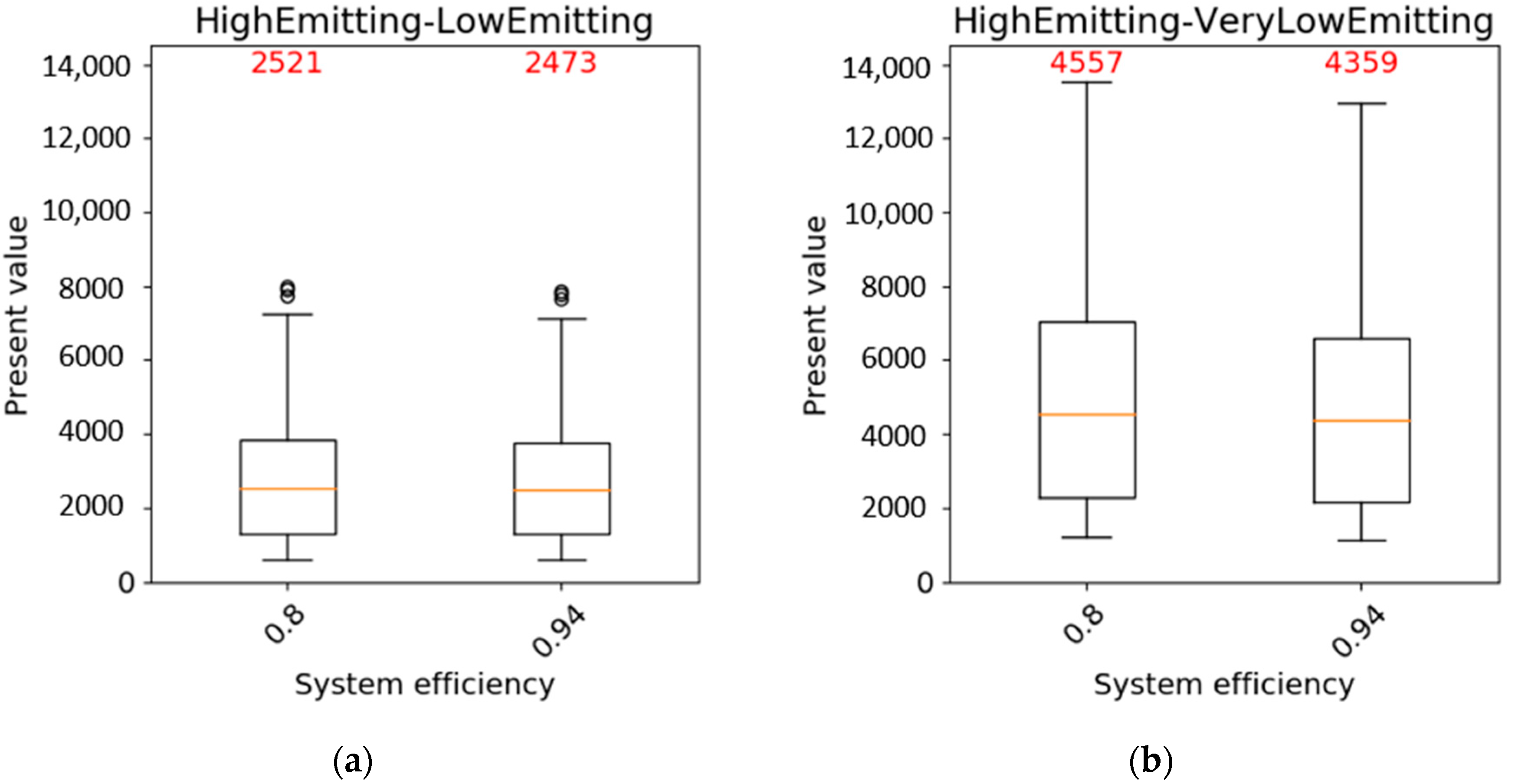
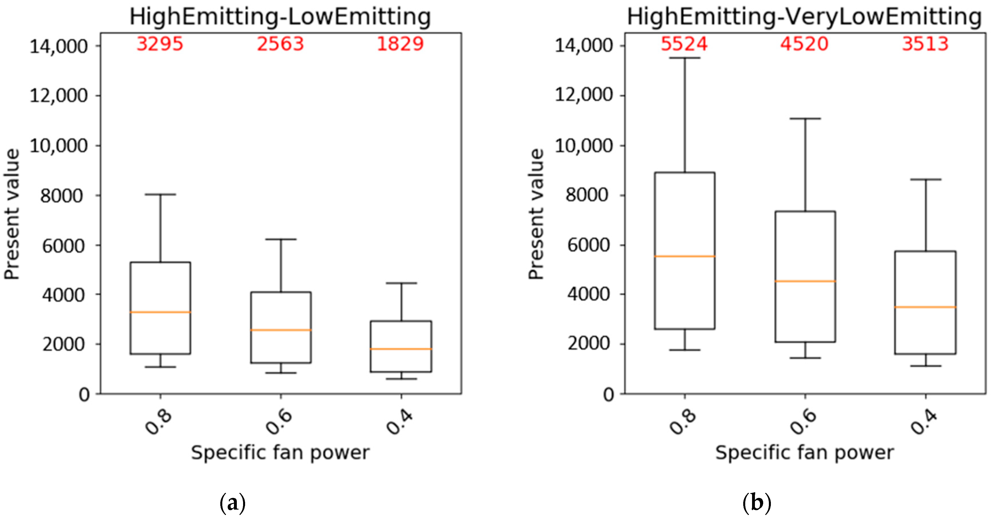
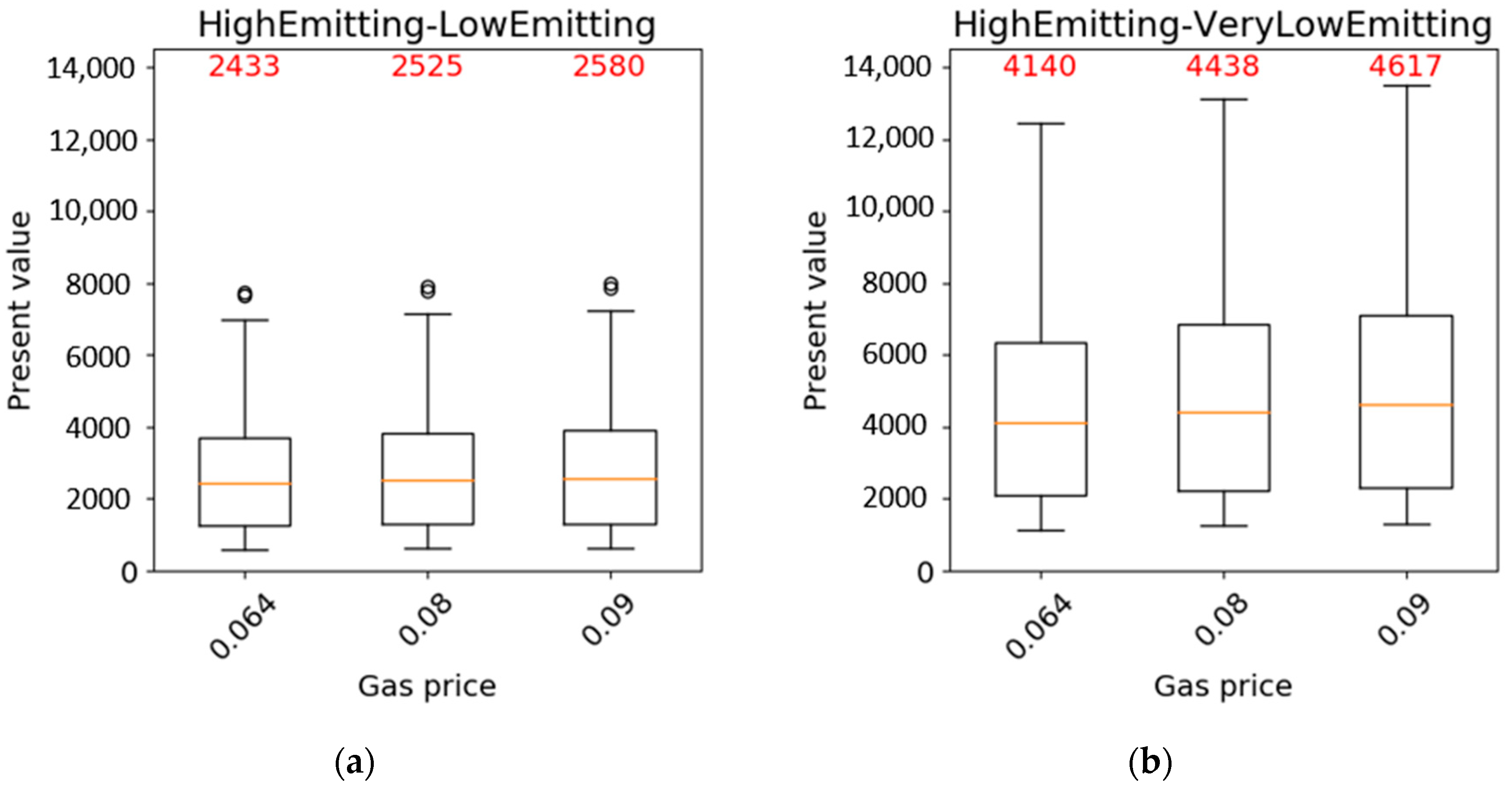
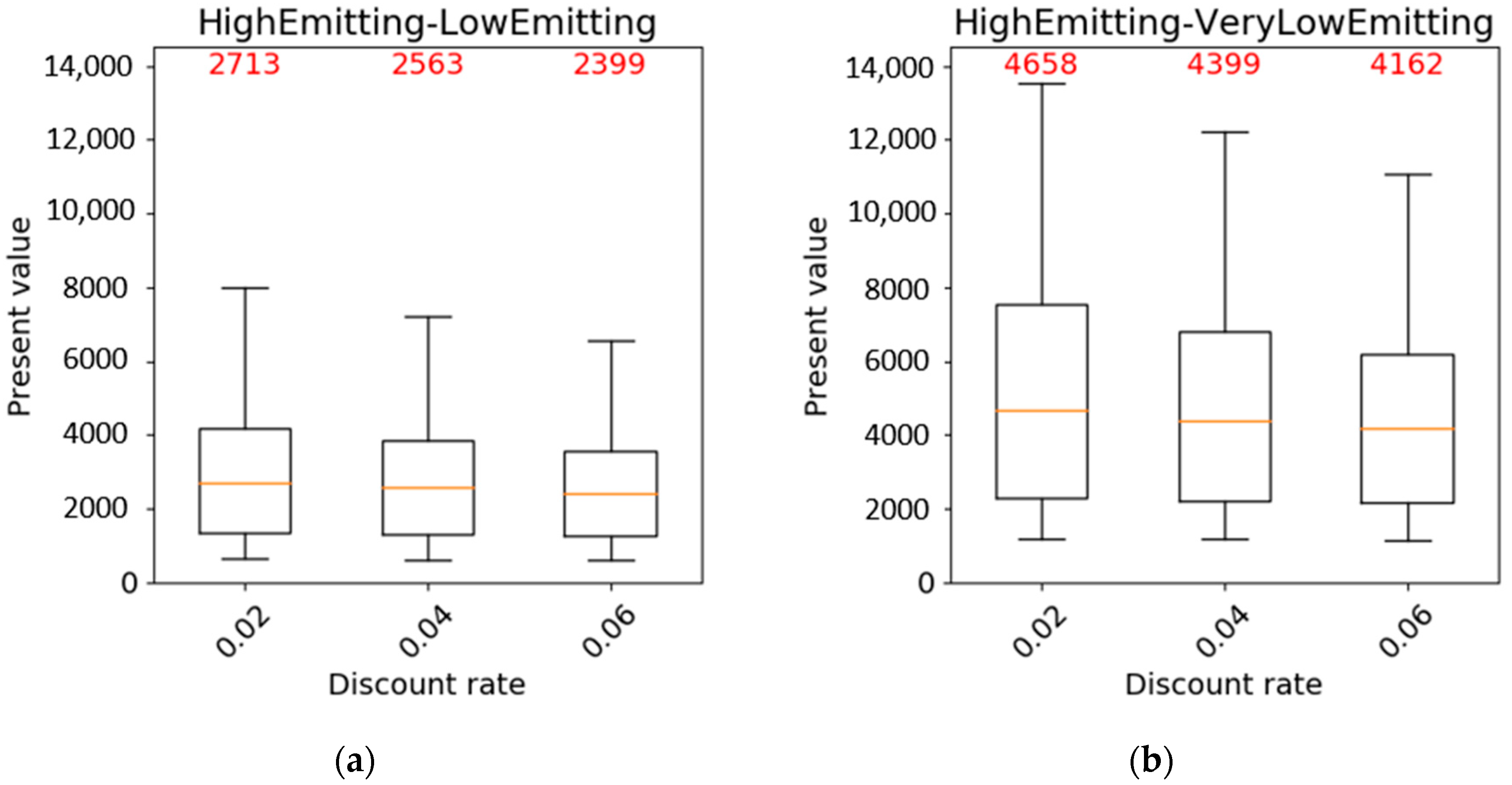
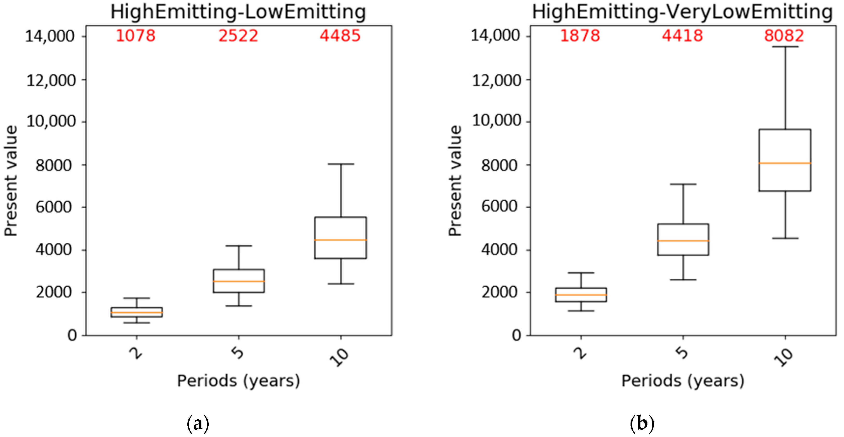
3.1. Results of the Cost–Benefit Analysis

The results are presented by comparing the output for the two scenarios depending on how the difference in energy consumption was calculated, namely (i) high emitting minus low emitting (HE − LE), and (ii) high emitting minus very low emitting (HE − VLE). Table 5 reports the different energy demand figures for the two scenarios.
Considering all possible 486 combinations for both HE − LE and HE − VLE options, the overall key economic results, namely the PV values, are presented in Table 6. As it can be seen from the table, the range is quite wide in both options, and the median is considerably lower than the maximum PV being closer to the minimum value. This suggests that, in general, savings are not negligible, but that the most relevant savings are achieved under a few configurations only.
The next step was an analysis of the disaggregated results to see the effect of the different input parameters on the present values. As shown in Figure 2, the efficiency of the heating system does not have a major impact on the PV. The difference between the two medians is lower than 2% and the distribution (displayed by means of boxplots) has a similar shape. Like the overall figures, in this case, there is also a significant difference between the HE − LE and HE − VLE scenario.
The specific fan power has a higher impact on the present value calculation compared to the heating system efficiency. As shown in Figure 3, more efficient fans lead to a 22% to 44% reduction in the median present value in the HE − LE scenario, and a 18% to 36% reduction in the HE − VLE scenario. In the latter, the percentage values are slightly lower, but the absolute difference is higher as the median values are higher. In general, the reasons for this higher impact are the fact that the difference between the three levels of specific fan power are proportionately wider than the difference between the efficiency levels used for the heating system, and the more elevated cost of electricity compared to gas.
Similarly, the present value is considerably less sensitive to variations (±20% variation in both cases) in the gas price (Figure 4) than in the electricity price (Figure 5) due to the fact that electricity is more expensive. For electricity, an increase in the unit price makes the median present value higher, but the distribution of the values also spreads, as shown by the increasing vertical dimension of the boxes (Figure 5) that encloses the values between the 25th and 75th percentiles for each distribution.
The two remaining variable parameters to be analyzed are the discount rate and the number of periods used for the PV calculation. Figure 6 shows that the higher the discount rate is, the lower the PV becomes. This is simply because the discount rate is used to move cashflows across a given time frame (i.e., the chosen number of periods) taking into account the fact that cashflows that happen in the far future have a lower value than cashflows nearer to the time of the analysis (i.e., time zero). As in this case all future cashflows are identical (sign and absolute value), an increase in the discount rate implies a decrease in their discounted sum, which is by definition the PV.
Lastly, Figure 7 highlights how the selection of a certain number of years is the most critical parameter. In the HE − LE scenario, the increase from 2 to 5 years leads to a median PV that is nearly 2.5 times higher (233% increase) while when considering 10 years, the PV becomes over 4 times higher (416%). A similar trend also happens in the HE − VLE scenario, although in this case, the absolute figures are more elevated. In both scenarios, the vertical dimension of the boxes (that shows how widely the values between the 25th and 75th percentile are spread) also grows with the number of years as the effect of the variations in the other parameters becomes increasingly relevant as more terms (i.e., annual cashflows) are added together.
To sum up, the PV calculation highlighted that the discounted value of the energy savings achieved by lower ventilation rates could potentially exceed 13,500€, which is money that could be spent at time zero to purchase low-polluting furniture or construction materials. The most critical and influencing parameter is the number of years followed by the variables linked to the electrical energy, namely its price and the specific fan power. On the other hand, variations in the variables related to gas consumption have very little impact on the final PV.

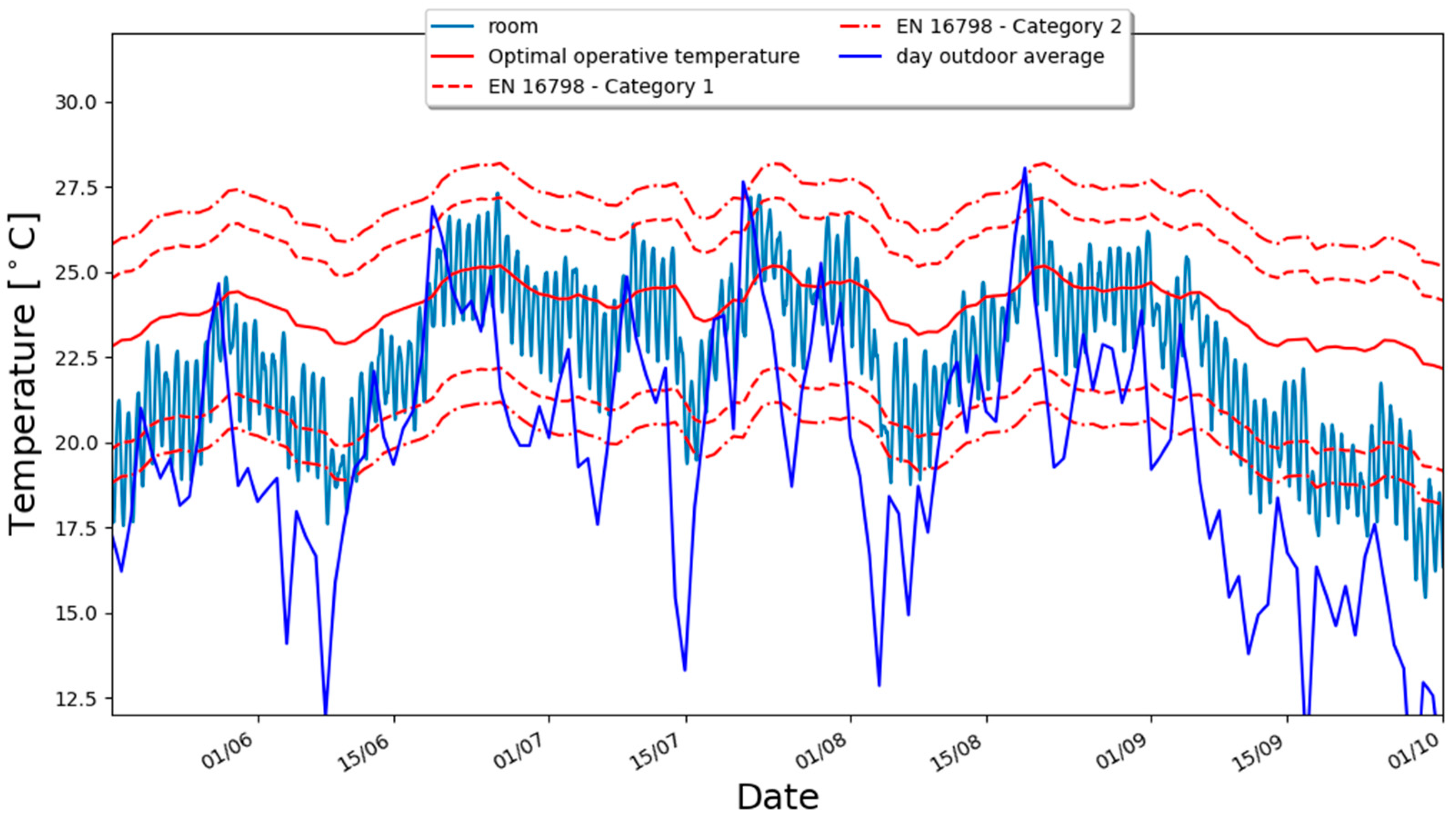
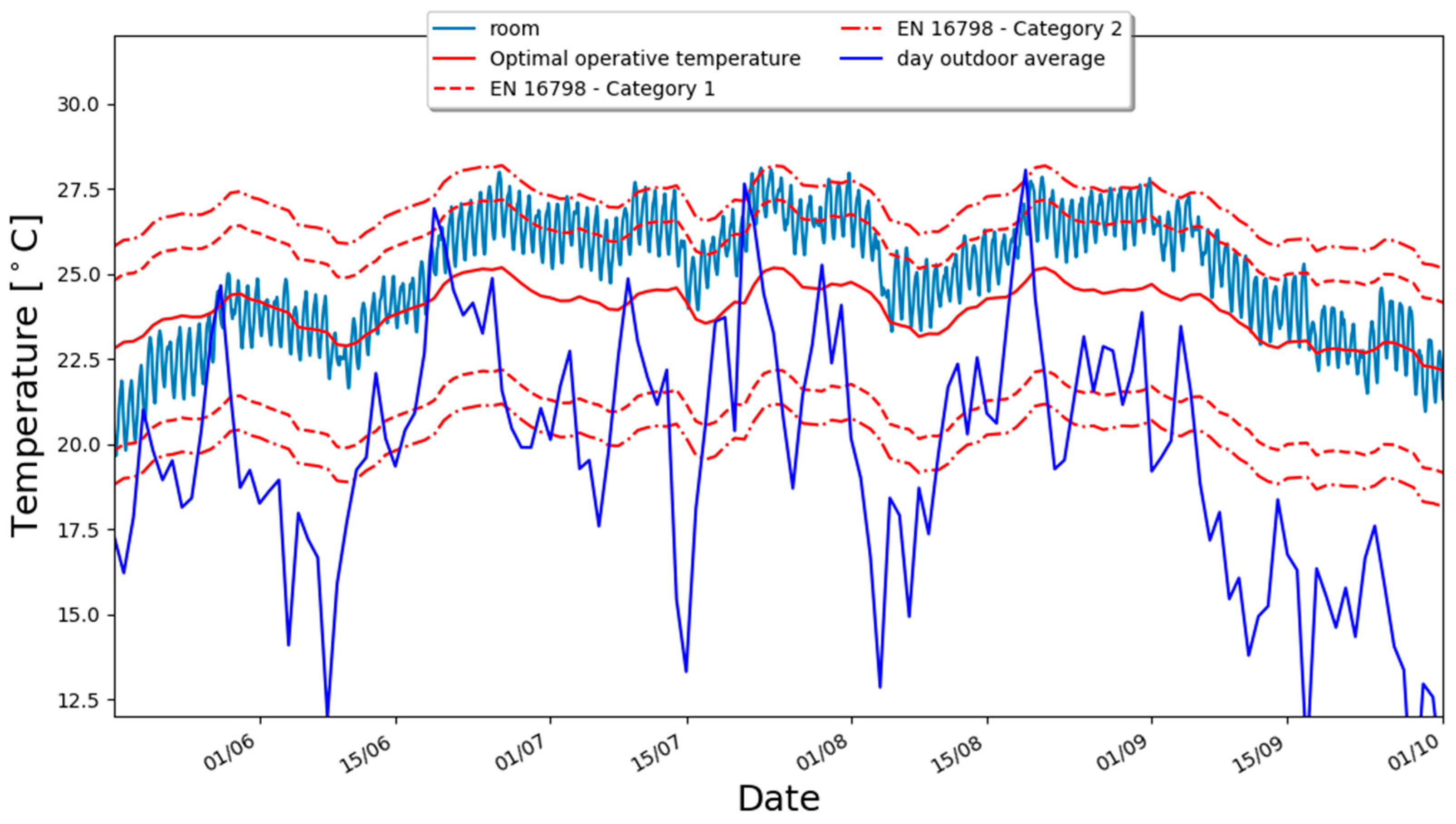
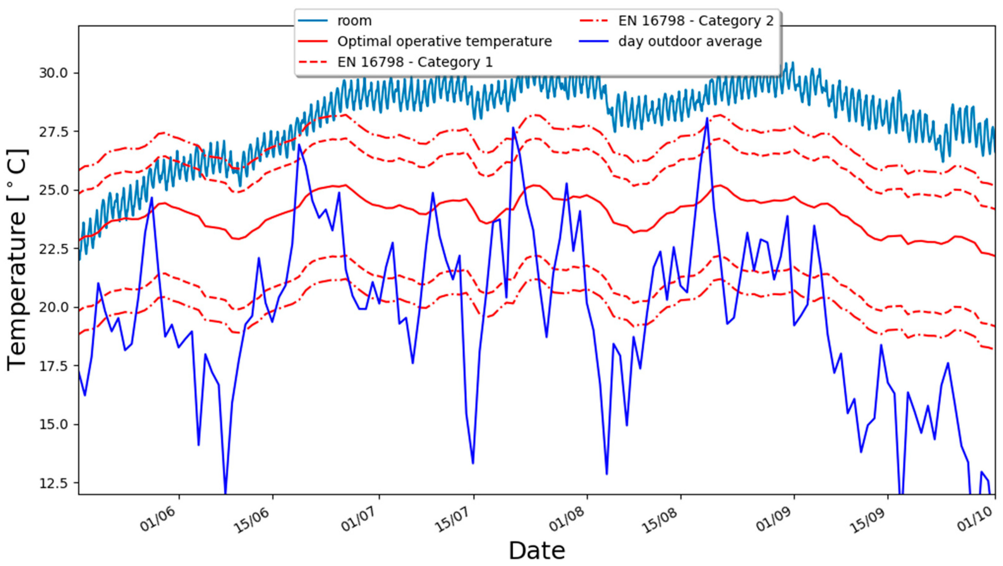
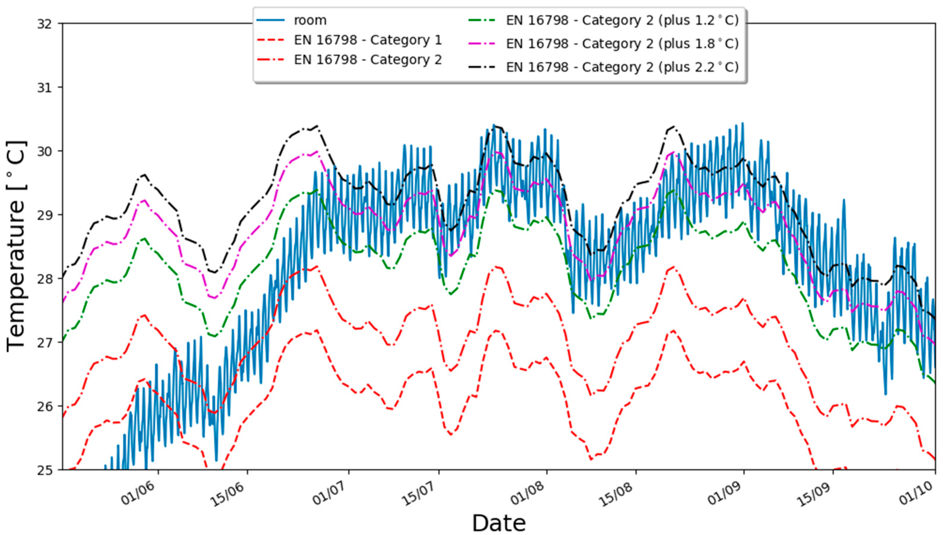
3.2. Thermal Comfort Analysis

The entire economic analysis was based on the assumption that the use of low-polluting materials enables a reduction of the ventilation rates, and this was converted into cashflows. Hence, the IAQ level in the three configurations (high emitting, low emitting, and very low emitting) was the same. However, this is not true for thermal comfort over the whole year. During the heating season, the variation in the ventilation rates resulted in a variation of the heating energy demand, but the level of thermal comfort is the same because of the ideal heating system and the same schedule setpoint. However, during the period from 15 May to 30 September, the simulation was run in free-floating mode and there was neither temperature control nor free cooling.
Figure 8, Figure 9 and Figure 10 show the temperature inside the living room in the three different configurations during the non-heating period, the outdoor temperature, and the temperature limits of category 1 and 2 of the standard EN16798:1 [17]. The closer the room temperature is to the optimal operative temperature, the higher the thermal comfort level is likely to be. For a residential building, the target limits suggested by the EN16798:1 are the category 2 limits.
As expected, the room temperature increases as the ventilation rates decrease. Considering the high-emitting and low-emitting configurations, this means that the room will usually be a little warmer, but the overall thermal comfort is enhanced. As shown in Figure 11 and Table 7, the number of hours in category 1 is nearly the same, with the difference being equal to 36 h (i.e., less than 1%), but the total number of hours in category 2 (lower plus upper parts) increases from 421 (12.8%) to 675 (20.5%). This is because in the low-emitting configuration, the total number of hours that are not in category 1 or 2 is reduced to 71 (2.2%). In other words, in none of the hours is the room too cold, and only in around 2% of the hours is it too warm. Moreover, Figure 9 shows that the category 2 upper limit is only slightly exceeded.
The very low-emitting scenario is instead considerably less comfortable. Without a cooling system, the reduction in the ventilation rates leads to a drop of the number of hours in category 1 down to 395 (12.0%), which is compensated by a spike in the number of hours above category 2 of over 80%. This means that for a large proportion of the time, the building is overheated, and Figure 10 highlights that the magnitude of this overheating is not negligible.

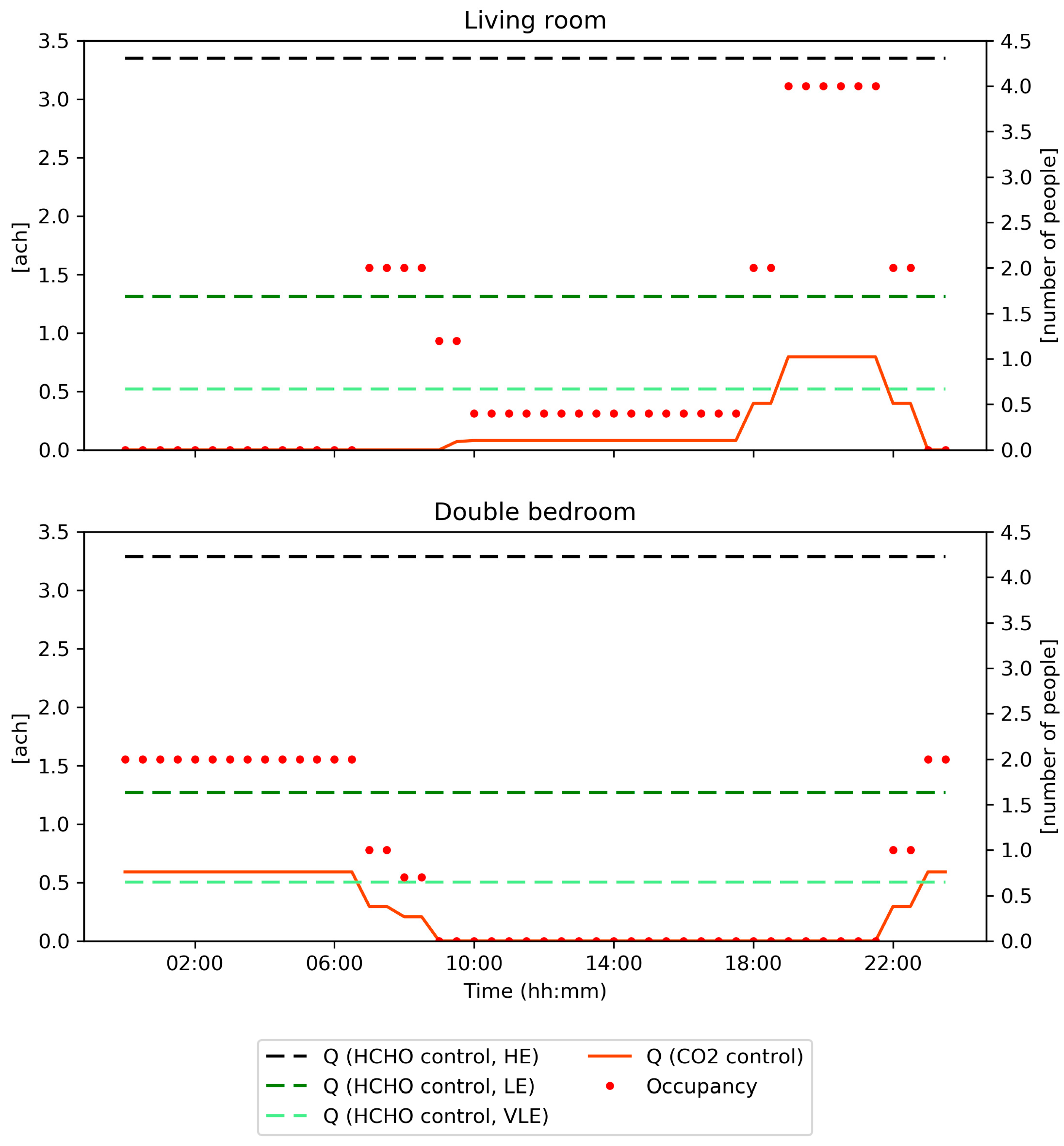
3.3. Comparison of the Required Ventilation Rates to Control Different Pollutants within the Room

In both standards and current practice, ventilation systems are sized and controlled on the basis of the CO2 concentration as the main indicator of all human-generated bio-effluents and indoor pollutants related to occupancy. However, this is very unlikely to be sufficient in several situations in which there are other pollutants not related to occupancy, such as formaldehyde. Figure 12 compares the ventilation rates needed to control the contaminant in the three building typologies (HE, LE, VLE), respectively, for the living room and the double bedroom. To keep the formaldehyde concentration below the guideline value, for the living room, 3.4 ach for HE, 1.3 ach for LE, and 0.5 ach for VLE are required, respectively, while lower and variable ventilation rates are needed to keep the CO2 concentration within the room below the guideline value. CO2-based ventilation rate requirements are zero or very low ventilation rates until 6 pm, where the living room’s occupancy is low, and reaches a maximum value of 0.8 ach when the room is occupied by four people. A similar behavior can be observed for the double bedroom. In this case, the air changes required to control the formaldehyde are 3.3 (HE), 1.3 (LE), and 0.5 ach (VLE) while the one needed to dilute the CO2 is lower due to the lower occupancy of the bedroom, and reaches a peak value of 0.6 ach when the room is occupied by two people. This gives evidence of the fact that the design and control of the ventilation rate based on the CO2 concentration only is usually not enough to guarantee a good air quality if other dominant pollutants, such as the formaldehyde, are present.

4. Discussion

The results of the cost–benefit analysis show that the potential savings range from a few hundred Euro to over 13,500€. This means that there could be a significant extra budget that could be spent at time zero to purchase less-emitting materials but that this would happen only under a few circumstances.
Considering the thermal comfort results during the warm season, the use of very low-emitting materials becomes less appealing. Unless a cooling system is installed, the building occupants would indeed experience a considerably overheated building. IAQ would be acceptable as the ventilation rates would be adequate to keep contaminants below harmful concentrations, but thermal comfort is not guaranteed for the largest part of the period from mid-May to the end of September.
Thermal comfort could be improved by adopting ventilated cooling strategies [25], which use the cooling capacity of outdoor air to reduce or even eliminate the cooling loads. This would result in temperature-controlled ventilation to increase the ventilation rate when the outdoor air has an effective cooling capacity.
A complementary solution to improve the thermal comfort is relying on air movement to improve thermal comfort during the warm season [26]. The EN16798:1 adaptive model does not include an explicit method for including air movement as done in other adaptive models, such as ASHRAE 55 [15] and the Indian model for adaptive comfort (IMAC) [27]. The former allows an increase of the acceptability upper limit according to the available air speed: 1.2 °C for 0.6 m/s, 1.8 °C for 0.9 m/s, and 2.2 °C for 1.2 m/s. The latter uses different equations in the presence of air movement. The ASHRAE 55 approach is explicit, and hence it might be applied to EN16798:1 limits as shown in Figure 13. However, this would not solve the thermal comfort issue for the whole period but would slightly increase both the capital cost and running costs, and it is questionable from a scientific perspective. The ASHRAE 55 and EN16798:1 equations are derived from different studies and based on different assumptions. Hence, further research is needed to assess whether the same set-point increases are valid for both models.
Another technically feasible solution is installing an air-conditioning system, such as a multi-split system, that would enable use of it only in a certain part of the building and when needed. However, this solution increases both the capital cost (to purchase the device) and the running costs, which are electivity costs, and hence would have a high impact on the PV calculation. Moreover, a major issue is the significant negative effect of this technology on global warming. Hence, the use of air conditioning should be discouraged from both a financial and environmental perspective.
If the VLE configuration is therefore not feasible for thermal comfort reasons, the maximum available extra budget at time zero (i.e., the maximum PV for the HE − LE scenario) is cut down to approximately 8000€. As a result, it seems that only the 10-year scenario has a median PV value of 4485€ (Figure 7), which enables a non-negligible upgrade of the materials. Considering furniture, there is an extremely wide range of products available on the market with very different prices. This extra budget might enable some improvements, but it is arguable that it is sufficient to use only low-emitting furniture for a house, such as this case study. This means that the total capital cost required to use only low-emitting materials is likely to be higher than 4485€ (and also than 8000€), and hence a pure cost–benefit analysis would not support this choice as the NPV would become negative.
However, the use of low-emitting materials leads to other benefits that are not considered in a cost–benefit analysis. Firstly, thermal comfort is enhanced and IAQ is similar to the HE scenario but using lower ventilation rates. This means that if, for any reasons, higher ventilation rates cannot be guaranteed, the house would still be thermally comfortable and healthy, being more resilient. This is a major advantage as the occupants of a comfortable and healthy house are more likely to be healthy too, generating a benefit for themselves and for society. Secondly, the use of a lower ventilation rate means less energy consumption, and hence a reduction of CO2 emissions, which is again a benefit for the whole society. Lastly, the disposal of low-emitting materials is also likely to be easier from an environmental point of view. All these points together can be classified as co-benefits, which could be monetized, but the methods to do so are complex and hence more studies are needed for an accurate evidence-based co-benefits analysis. This analysis would explain why and the extent to which people are willing to accept an extra cost for having a better indoor (IEQ) and outdoor (less CO2 emitted and fewer contaminants released from houses to the atmosphere) environment. Field studies are essential to build a robust framework for the co-benefits’ evaluation.
In South Tyrol, according to the database of the local energy certification agency Agenzia per l’Energia Alto Adige–CasaClima (this database is not public and it can be accessed via the agency only), over 60% of new buildings built in 2016 and 2017 were single- or double-family houses. Therefore, the study focused on this building typology. Due to the large floor area per person available in single-family houses, the results cannot be directly extended to other building typologies, such as apartments, since these are characterized by an elevated occupant density within the residential unit, and therefore by higher CO2 concentrations. However, the results of this study are applicable to recent and new single- and double-family houses located in the Mediterranean and continental climate with a number of degree days between 2100 and 3000 (called zone E in the Italian climatic zones’ definition).

5. Conclusions

This research presented a cost–benefit analysis of the IAQ in residential buildings using a case-study building, and three sets of materials with different pollution emission levels, namely high, low, and very low emitting. The main conclusions of this study are as follows.
  • Depending on the scenario, the use of low- and very low-emitting materials enables an up to 13,500€ running cost reduction over a 10-year period, which results in extra in the budget that could be used to purchase these higher quality materials.
  • In the cost–benefit analysis, the variables that have the largest effect on the present value are the number of periods (i.e., years) and those related to electricity (cost and efficiency).
  • In Bolzano climatic conditions, the use of a ventilation strategy based only on IAQ does not ensure the thermal comfort requirements are met during summer unless some cooling strategies are adopted.
  • An analysis of the co-benefits is essential to fully understand why and the extent to which people are willing to accept extra costs to have a better indoor and outdoor environment.
There are also some main limitations of this study. Firstly, the analysis could be conducted on a larger sample of building archetypes. Secondly, natural ventilation was not considered, but further work should consider this possibility as it is widely used in South Tyrol. Thirdly, in residential buildings, indoor and outdoor noise and sound also affect the use of ventilation devices and openings, but this aspect was not included in this research. Then, in the financial analysis, inflation was not considered as its value has been very low in recent years. This might not be true in longer term projects. Finally, in this study, it was assumed that materials have the same emission rates throughout their lifetime. Anecdotal evidence suggests that this is not the case, but further work is needed to characterize the long-term emission rate and the facts that modify it (e.g., time, direct sunlight exposure).

Author Contributions

Conceptualization, F.B. and I.D.; methodology, F.B, I.D. and A.B.; software, F.B., I.D., A.B. and F.A.; formal analysis, F.B. and I.D.; writing—original draft preparation, F.B., I.D., A.B. and F.A.; writing—review and editing, F.B.; visualization, F.B., I.D. and F.A.; supervision, F.B. and A.B.; project administration, F.B.; funding acquisition, F.B. All authors have read and agree to the published version of the manuscript.

Funding

The research leading to these results has received funding from the European Regional Development Fund POR FESR 2014–2020 of the Province of Bolzano, under Project number 1116, NEW-AIR: Nuovo approccio per una qualità degli ambienti interni energeticamente efficiente: ricerca e aziende fanno sistema in Alto Adige (In English: New approach for an energy efficient indoor environmental quality: research and firms make system in South Tyrol).

Acknowledgments

The authors would like to thank the Province of Bolzano for its financial support.

Conflicts of Interest

The authors declare no conflict of interest.

References

  1. Klepeis, N.; Nelson, W.C.; Ott, W.R.; Robinson, J.P.; Tsang, A.M.; Switzer, P.; Behar, J.V.; Hern, S.C.; Engelmann, W.H. The National Human Activity Pattern Survey (NHAPS): A Resource for Assessing Exposure to Environmental Pollutants. J. Expo. Sci. Environ. Epidemiol. 2001, 11, 231–252. [Google Scholar] [CrossRef] [PubMed] [Green Version]
  2. Eurostat. Manual for Statistics on Energy Consumption in Households; Publications office of the European Union: Luxembourg, 2013.
  3. ASHRAE. Standard 62.1—Ventilation for Acceptable Indoor Air Quality; ASHRAE: Atlanta, GA, USA, 2016. [Google Scholar]
  4. WHO Global Health Observatory (GHO) Data. Available online: https://www.who.int/gho/phe/en/ (accessed on 5 November 2019).
  5. Abadie, M.; Wargocki, P.; Rode, C.; Zhang, J. General rights Proposed metrics for IAQ in low-energy residential buildings. ASHRAE J. 2019, 61, 62–65. [Google Scholar]
  6. Abadie, M.O.; Wargocki, P.; Rode, C.; Rojas-Kopeinig, G.; Kolarik, J.; Laverge, J.; Cony, L.; Qin, M.; Blondeau, P. Indoor Air Quality Design and Control in Low-Energy Residential Buildings-Annex 68 | Subtask 1: Defining the Metrics in the Search of Indices to Evaluate the Indoor Air Quality of Low-Energy Residential Buildings; IEA-EBC: Birmingham, UK, 2017. [Google Scholar]
  7. Gibson, G.J.; Loddenkemper, R.; Lundbäck, B.; Sibille, Y. Respiratory health and disease in Europe: the new European Lung White Book. Eur. Respir. J. 2013, 42, 59–563. [Google Scholar] [CrossRef] [PubMed]
  8. Salthammer, T. Data on formaldehyde sources, formaldehyde concentrations and air exchange rates in European housings. Data Br. 2019, 22, 400–435. [Google Scholar] [CrossRef] [PubMed]
  9. WHO. WHO Guidelines for Indoor Air Quality: Selected Pollutants; Regional Office for Europe: Copenhagen, Denmark, 2010. [Google Scholar]
  10. Walker, I.; Sherman, M.; Jones, B. Economics of Indoor Air Quality. In Proceedings of the 39th AIVC Conference “Smart Ventilation for Buildings”, Antibes Juan-Les-Pins, France, 18–19 September 2018; pp. 1–9. [Google Scholar]
  11. Guyot, G.; Sherman, M.H.; Walker, I.S. Smart ventilation energy and indoor air quality performance in residential buildings: A review. Energy Build. 2018, 165, 416–430. [Google Scholar] [CrossRef] [Green Version]
  12. Rakennustietosäätiö RTS sr. M1 Emission Classification of Building Materials: Protocol for Chemical and Sensory Testing of Building Materials; Finnish Building Information Foundation RTS sr: Helsinki, Finland, 2017. [Google Scholar]
  13. NIST ContamLink | NIST. Available online: https://www.nist.gov/el/energy-and-environment-division-73200/nist-multizone-modeling/software-tools/contamlink (accessed on 10 October 2019).
  14. Brown, S.K. Chamber Assessment of Formaldehyde and VOC Emissions from Wood-Based Panels. Indoor Air 1999, 9, 209–215. [Google Scholar] [CrossRef] [PubMed]
  15. ASHRAE. Standard 55 - Thermal Environmental Conditions for Human Occupancy; ASHRAE: Atlanta, GA, USA, 2017. [Google Scholar]
  16. ASHRAE. Handbook of Fundamentals; ASHRAE: Atlanta, GA, USA, 2013. [Google Scholar]
  17. CEN. EN 16798-1 - Energy Performance of Buildings - Ventilation for Buildings - Part 1: Indoor Environmental Input Parameters for Design and Assessment of Energy Performance of Buildings Addressing Indoor Air Quality, Thermal Environment, Lighting and Acoustic; European Standard: Bruxelles, Belgium, 2019. [Google Scholar]
  18. CEN. CEN/TR 16798-2 - Energy Performance of Buildings - Ventilation for Buildings - Part 2: Interpretation of the Requirements in EN 16798-1; European Standard: Bruxelles, Belgium, 2019. [Google Scholar]
  19. IEE TABULA - Typology Approach for Building Stock Energy Assessment. Available online: https://ec.europa.eu/energy/intelligent/projects/en/projects/tabula (accessed on 1 September 2019).
  20. Wilson, E.; Engebrecht-Metzger, C.; Horowitz, S.; Hendron, R. 2014 Building America House Simulation Protocols; National Renewable Energy Lab (NREL): Denver, CO, USA, 2014.
  21. UNI UNI/TS 11300-2 - Prestazioni energetiche degli edifici - Parte 2: Determinazione del fabbisogno di energia primaria e dei rendimenti per la climatizzazione invernale, per la produzione di acqua calda sanitaria, per la ventilazione e per l’illuminazione in; UNI: Milano, Italy, 2019.
  22. Merzkirch, A.; Maas, S.; Scholzen, F.; Waldmann, D. Field tests of centralized and decentralized ventilation units in residential buildings – Specific fan power, heat recovery efficiency, shortcuts and volume flow unbalances. Energy Build. 2016, 116, 376–383. [Google Scholar] [CrossRef]
  23. Eurostat Natural Gas Price Statistics - Statistics Explained. Available online: https://ec.europa.eu/eurostat/statistics-explained/index.php?title=Natural_gas_price_statistics (accessed on 31 October 2019).
  24. Eurostat Electricity Price Statistics - Statistics Explained. Available online: https://ec.europa.eu/eurostat/statistics-explained/index.php?title=Electricity_price_statistics (accessed on 31 October 2019).
  25. Heiselberg, P.; O’Donnavan, A.; Belleri, A.; Flourentzou, F.; Zhang, G.-Q.; Carrilho da Graca, G.; Breesch, H.; Justo-Alonso, M.; Kolokotroni, M.; Pomianowski, M.; et al. Ventilative Cooling Design Guide - IEA Annex 62 Report; IEA-EBC: Birmingham, UK, 2018. [Google Scholar]
  26. Babich, F.; Cook, M.J.; Loveday, D.L.; Rawal, R.; Shukla, Y. A new methodological approach for estimating energy savings due to air movement in mixed mode buildings. In Proceedings of the IBPSA, San Francisco, CA, USA, 7–9 August 2017. [Google Scholar]
  27. Manu, S.; Shukla, Y.; Rawal, R.; Thomas, L.E.; De Dear, R. Field studies of thermal comfort across multiple climate zones for the subcontinent: India Model for Adaptive Comfort (IMAC). Build. Environ. 2016, 98, 55–70. [Google Scholar] [CrossRef] [Green Version]
Figure 1. The case-study building. (a) Tridimensional model; (b) first floor (north is on top); (c) ground floor. The red line indicates an adiabatic wall (adjacent building).
Atmosphere 11 00102 g001
Figure 2. Present values in Euros calculated with different heating system efficiency values: 0.80 indicates a less efficient system (e.g., traditional non-condensing boiler) while 0.94 a very efficient heating system (e.g., condensing boiler and state-of-the-art set-up). The red numbers indicate the median value. (a) Scenario HE − LE. (b) Scenario HE − VLE. High-emitting (HE), low-emitting (LE).
Atmosphere 11 00102 g002
Figure 3. Present values calculated with different specific fan power: the lower this value is, the more efficient the fans are. (a) Scenario HE − LE. (b) Scenario HE − VLE.
Atmosphere 11 00102 g003
Figure 4. Present values calculated with different gas prices. (a) Scenario HE − LE. (b) Scenario HE − VLE.
Atmosphere 11 00102 g004
Figure 5. Present values calculated with different electricity prices. (a) Scenario HE − LE. (b) Scenario HE − VLE.
Atmosphere 11 00102 g005
Figure 6. Present values calculated with different discount rates. (a) Scenario HE − LE. (b) Scenario HE − VLE.
Atmosphere 11 00102 g006
Figure 7. Present values calculated with different numbers of periods (in this case, years). (a) Scenario HE − LE. (b) Scenario HE − VLE.
Atmosphere 11 00102 g007
Figure 8. Temperature in the living room during the non-heating season; high-emitting configuration.
Atmosphere 11 00102 g008
Figure 9. Temperature in the living room during the non-heating season; low-emitting configuration.
Atmosphere 11 00102 g009
Figure 10. Temperature in the living room during the non-heating season; very low-emitting configuration.
Atmosphere 11 00102 g010
Figure 11. Distribution of the hours from 15 May to 30 September in the EN16798:1 categories for the three configurations: (a) high emitting, (b) low emitting, and (c) very low emitting.
Atmosphere 11 00102 g011
Figure 12. Required ventilation rates to maintain CO2 and formaldehyde concentration below the guideline values for the living room and the double bedroom.
Atmosphere 11 00102 g012
Figure 13. Temperature in the living room during the non-heating season with the category 2 limit extended to consider elevated air movement; very low-emitting configuration.
Atmosphere 11 00102 g013
Table 1. Formaldehyde emission rates for different emission classes. HE: high-emitting, LE: low-emitting, VLE: very low-emitting.
Building Material Emission ClassFormaldehyde EmissionUnits
HE building320µg/(m2h)
LE building125µg/(m2h)
VLE building50µg/(m2h)
Table 2. Characteristics of the construction element.
ElementsDescriptionThickness (m)U-Value (W/m2K)
exterior wallmassive wall with external insulation0.490.18
roofwooden roof isolated with wood fiber0.330.14
ground floorconcrete slab with insulation0.1650.165
windowtriple glazing window with argon and wooden frame0.0840.49
(Ug = 0.6 Uf = 1.2)
Table 3. Air change rate scheduled in each building model and the maximum CO2 and formaldehyde concentration calculated.
Case-Study BuildingLiving RoomDouble Bedroom
Air Change Rate (1/h)Max CO2 Concentration (ppm)Max HCHO Concentration (µg/m3)Air Change Rate (1/h)Max CO2 Concentration (ppm)Max HCHO Concentration (µg/m3)
HE3.4573283.353128
LE1.3822281.373928
VLE0.5–0.81126280.5–0.6117429
Table 4. Economic analysis input values.
ParametersValuesUnits
Heating system efficiency80, 94%
Specific fan power0.40, 0.60, 0.80Wh/m3
Electricity price0.17, 0.21, 0.25€/kWh
Gas price0.06, 0.08, 0.10€/kWh
Discount rate2, 4, 6%
Years2, 5, 10years
Table 5. Difference in energy demand.
VariableScenario HE − LEScenario HE − VLEUnits
Heating demand9133738kWh/year
Electricity demand39165392kWh/year
Table 6. Overall economic results.
Present ValueScenario HE − LEScenario HE − VLEUnits
Median24934418
Mean27814910
Maximum800913,524
Minimum5961130
Table 7. Number of hours from 15 May to 30 September in the EN16798 categories for the three configurations (absolute and percentage figures).
EN16798 CategoryHigh EmittingLow EmittingVery Low Emitting
Below category 2359 (10.9%)0 (0.0%)0 (0.0%)
Category 2-lower part381 (11.6%)7 (0.2%)0 (0.0%)
Category 12507 (76.2%)2543 (77.3%)395 (12.0%)
Category 2-upper part40 (1.2%)668 (20.3%)257 (7.8%)
Above Category 22 (0.1%)71 (2.2%)2637 (80.2%)

