Article

Evolution of Turbulence in the Kelvin–Helmholtz Instability in the Terrestrial Magnetopause

by
Francesca Di Mare
1,*,
Luca Sorriso-Valvo
2,3,
Alessandro Retinò
4,
Francesco Malara
5 and
Hiroshi Hasegawa
6
1
Department of Physics, University of Oslo, 1048 Blindern, 0316 Oslo, Norway
2
Departamento de Física, Escuela Politécnica Nacional, Av. Ladrón de Guevara E11–253, 170517 Quito, Ecuador
3
ISTP/CNR, U.O.S. di Bari, Via Amendola, 122/D 70126 Bari, Italy
4
Laboratoire de Physique des Plasmas, CNRS/Ecole Polytechnique/Sorbonne Université/Université Paris Sud/Observatoire de Paris, route de Saclay, F-91128 Palaiseau, France
5
Dipartimento di Fisica, Università della Calabria, Ponte P. Bucci, cubo 31C, 87036 Rende, Italy
6
Institute of Space and Aeronautical Science, JAXA, 3-1-1 Yoshinodai, Chuo, Sagamihara, Kanagawa 252-5210, Japan
*
Author to whom correspondence should be addressed.
Atmosphere 2019, 10(9), 561; https://doi.org/10.3390/atmos10090561
Submission received: 12 August 2019 / Revised: 10 September 2019 / Accepted: 11 September 2019 / Published: 18 September 2019

Abstract

:
The dynamics occurring at the terrestrial magnetopause are investigated by using Geotail and THEMIS spacecraft data of magnetopause crossings during ongoing Kelvin–Helmholtz instability. Properties of plasma turbulence and intermittency are presented, with the aim of understanding the evolution of the turbulence as a result of the development of Kelvin–Helmholtz instability. The data have been tested against standard diagnostics for intermittent turbulence, such as the autocorrelation function, the spectral analysis and the scale-dependent statistics of the magnetic field increments. A quasi-periodic modulation of different scaling exponents may exist along the direction of propagation of the Kelvin–Helmholtz waves along the Geocentric Solar Magnetosphere coordinate system (GSM), and it is visible as a quasi-periodic modulation of the scaling exponents we have studied. The wave period associated with such oscillation was estimated to be approximately 6.4 Earth Radii ( R E ). Furthermore, the amplitude of such modulation seems to decrease as the measurements are taken further away from the Earth along the magnetopause, in particular after X ( G S M ) 15 R E . The observed modulation seems to persist for most of the parameters considered in this analysis. This suggests that a kind of signature related to the development of the Kelvin–Helmholtz instabilities could be present in the statistical properties of the magnetic turbulence.

1. Introduction

Turbulence at the interface between the solar wind and the magnetosphere is an important subject in space physics. Properties of turbulence can help with understanding the transport of mass, momentum, and energy from the solar wind to the magnetosphere [1,2] and, more generally, the mechanisms of interaction between these two regions of the near-Earth space.
The Kelvin–Helmholtz Instability (KHI) can drive waves at the magnetopause. These waves can grow to form rolled-up vortices and facilitate transfer of plasma into the magnetosphere. This mechanism is considered one of the most important in the low-latitude boundary layer (LLBL) during periods of northward Interplanetary Magnetic Field (IMF) [3], when reconnection at the equatorial magnetopause is less effective [4,5]. The Kelvin–Helmholtz instability can grow at the low-latitude magnetopause, situated between the magnetosheath, characterized by an anti-sunward flow of shocked solar wind, and the outer plasma sheet characterized by stagnant or weak sunward flows [6]. When the IMF is northward, the equatorial component of the magnetic field can be negligible at low latitude and so the KHI can develop eventually producing fully rolled-up vortices. There is an extensive literature for understanding development of this instability along the inner edge of the LLBL [7,8]. The resulting waves or vortices are suggested to have some relation to aurorae with spatially periodic forms [9,10]. There are observational evidence of the KHI in the form of surface waves propagating anti-sunward along the magnetopause [7,11,12,13]. A shared point of view considers Kelvin–Helmholtz waves or vortices to be more frequent during northward IMF conditions than during southward IMF [13,14,15]. Those vortices are believed to be a key ingredient for the formation of the thick LLBL [3] and of the cold and dense plasma sheet (CDPS) [16,17], both encountered predominantly under northward IMF. Kelvin–Helmholtz waves are known to develop at a planetary magnetopause, where small scale perturbations gain energy from the velocity shear between the magnetospheric and magnetosheath plasma and thereby grow into large scale rolled up vortices [18]. When the waves reach a turbulent state, plasma and energy are transported from the dense magnetosheath into the more rarified magnetosphere [19]. There is a lot of observational evidence to demonstrate the presence of Kelvin–Helmholtz waves on both the dawn and dusk flank of the terrestrial magnetosphere spanning approximately from the dawn–dusk meridian to 30 Earth radii down the magnetotail [12,14,20,21,22,23,24,25]. It looks like that the events arise in the proximity of the equatorial plane, where the magnetopause is believed to be susceptible to the KHI [23,26].
The KHI can also drive the turbulence in the magnetosheath region [11,12,21,23,24,25,27]. It is therefore interesting to study the characteristics of turbulence in the KHI regions, trying to understand the relationship between the instability and the various characteristics of turbulence such as power-law spectra and intermittency. To this aim, we analyzed the statistical properties of turbulence from a collection of Geotail observations, spanning nine years from 1995 to 2003. These events have been previously selected and studied by Fairfield et al. [12], Hasegawa et al. [15], Fujimoto et al. [28], Stenuit et al. [29]. To enrich the dataset, two additional events from THEMIS observations during November 2008, previously studied by Lin et al. [30], have been investigated. All events are encountered along the flank magnetopause, most of which are behind the dawn–dusk terminator, showing quasi-periodic plasma and field fluctuations in the flank low-latitude boundary layer under northward IMF, associated with Kelvin–Helmholtz waves. In Section 2, we present the dataset used for the analysis; in Section 3, we analyse the properties of turbulence, such as the autocorrelation function, the spectrum and the scale-dependent statistics of the field increments; in Section 4, we study the evolution of turbulence along the KHI; finally, in Section 5, we comment on the results obtained.

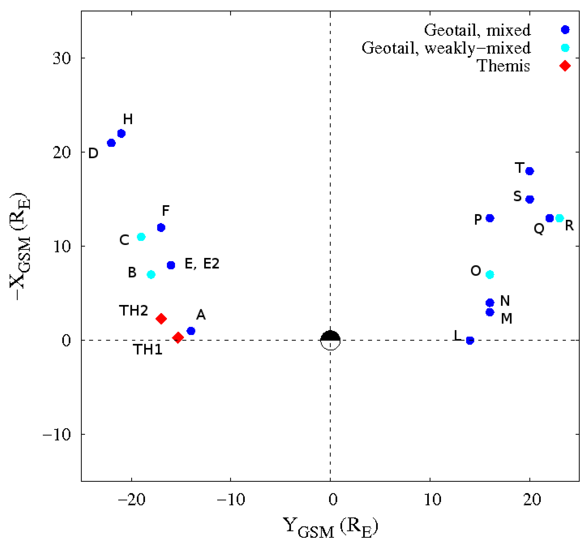
2. The Data: Geotail and THEMIS Magnetopause Crossing
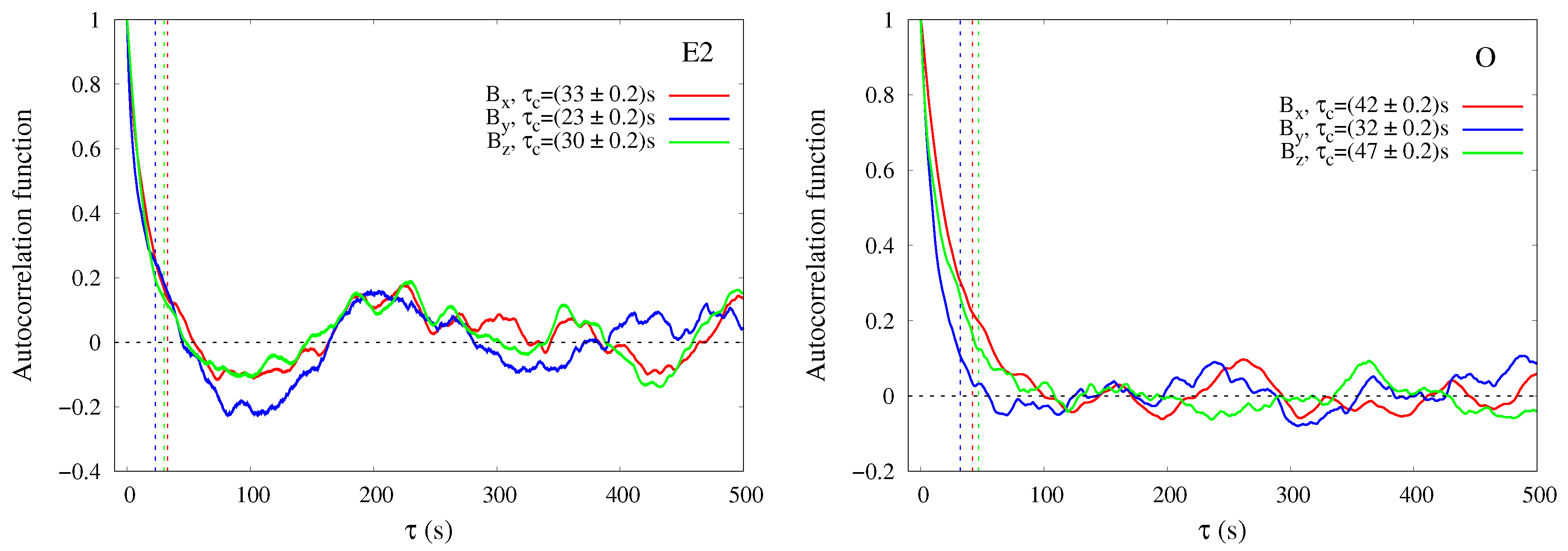
The description of the properties of turbulence is customarily performed through the high-order statistical analysis of the field increments. This requires that each interval should have a statistically significant number of measurements. As a rule of thumb, the correct estimate of the qth order moment requires 10 q measurements in order to ensure convergence. Based on this, in order to enable the computation of the fourth-order moments, we have selected a set of intervals each including a number of data points N 10 4 . Furthermore, we used intervals that are not affected by an excessive presence of data gaps, so that missing points are less than 10 % . According to these requirements, we have selected 17 Geotail events from the list of 19 reported by Hasegawa et al. [15]. Only two THEMIS events from the set of 14 reported by Lin et al. [30] have been chosen as the only ones with an interesting position for our analysis, i.e., behind the dawn–dusk terminator on the left-side where we have fewer Geotail events. The observed condition of all events are listed in Table 1 and in Table A1 in Appendix A. Table 1 shows the following information (from Hasegawa et al. [15]): date; time interval; GSM position measured in units of the Earth radius R E ; IMF condition; ion mixing status; fluctuation period, related to the rolled-up vortices; magnetosheath mean bulk velocity v m s ; wavelength λ , obtained multiplying the magnetosheath flow speed by the fluctuation period, and dividing by 1 R E . The ion mixing status is defined “mixed” if a significant amount of cool magnetosheath-like ions was present on the magnetospheric side of the magnetopause, where the density, evaluated using the full phase space distribution, is n > 1 /cm3; or “weakly-mixed”, when magnetosheath-like ions were found on magnetospheric side, with density lower than n < 1/cm3. The fluctuation period corresponds to the perturbations in the flow that are interpreted by Hasegawa et al. [15] as being due to vortical motions of plasma (e.g., Fujimoto et al. [14]), whereas those in the magnetic field are due to deformation of the field lines when those near the magnetopause are brought into rolled-up vortices [23,31]. The event recorded on 25 March 2002 (event F) is split into two different sets F a and F b because it presents a large gap in its central part.
The locations of all the selected events are presented in Figure 1. As can be seen, most of the events are behind the dawn–dusk terminator, and, more precisely: nine on the dawn-side (left-side in Figure 1) and nine on the dusk-side (right-side in Figure 1). Events E and E2 present the same X and Y (GSM) coordinates, so they are over-plotted on top of each other. From now on, we refer to the GSM coordinates with X, Y and Z in capital letters and for the magnetic field component in the same direction with x, y, z in lower case letters. Before proceeding to the analysis of the turbulence properties of the data, it is necessary to test the validity of the Taylor hypothesis, which allows the switch between time and space measurements [32]. In particular, the time series of a field can be assumed to be an instantaneous spatial scan of the field if the typical velocities associated with the dynamics are slower than the probe speed inside the medium. To be more precise, for a turbulent distribution of modes in wavevector space, the plasma-frame frequency term ω and spatial advection term k · v ms , (where v m s is the mean speed of each sample and the subscript “ms” indicates “magnetosheath” region, where our dataset is located), both contribute to the spacecraft-frame frequency [33], according to the relation [32]:
ω s c = ω + k · v ms .
As stated above, assuming ω k v A , and for a super-Alfvénic flow, v m s v A , then Equation (1) would imply ω s c k · v m s , thereby relating the spacecraft-frame frequency directly to the wavenumber of spatial fluctuations. This would correspond to the Taylor hypothesis [32,34].
In order to test the validity of the Taylor hypothesis in the samples studied here, values of the magnetosheath mean bulk speed and of the Alfvén speed were estimated for each interval under study. Unfortunately, their values are of the same order for almost all of the samples, so that the Taylor hypothesis does not hold, as shown in Table 2. However, it is possible to invoke a phenomenological approximation as an alternative to the Taylor hypothesis, previously presented by Stawarz et al. [35], and utilized in other magnetospheric studies of turbulence [36,37]. These authors assume that fluctuations are mainly Alfvénic (at least in the large-scale domain), so that their frequency in the plasma frame can be estimated as ω k · v A = k v A cos θ , where θ is the angle between k and B 0 . Indicating by ϕ the angle between k and v m s , the advection term is k · v m s = k v m s cos ϕ . Since in our samples v m s v A , the advection term dominates over the frequency term (thus allowing space-time conversion in the time series) only when cos θ cos ϕ , it is well known that, in magnetohydrodynamic (MHD) turbulence, the energy cascade tends to develop in the directions perpendicular to the mean magnetic field B 0 , so that perpendicular wave-vectors k dominate over parallel wave-vectors k | | . Thus, we can expect that θ is close to π / 2 . Examining our data, we verified that the mean magnetic field B 0 is mainly oriented in the z-direction (in GSM coordinates), therefore k is essentially in the x y plane. Instead, the plasma bulk velocity v m s is in the x-direction, i.e., mainly perpendicular to B 0 . This is confirmed by calculating the angle α between B 0 and v m s as
α = arccos B 0 · v ms | B 0 | | v ms | ,
which is consistently close to 90 for all samples (Table 2). This implies that the condition cos θ cos ϕ is satisfied in our database, so that the argument given by Stawarz et al. [35] holds, and the time series can be interpreted in terms of spatial measurements.
For the present analysis, we used the magnetic field time series sampled at d t = 0.0625 s obtained by the ASCII listings of Geotail MGF (Magnetic Field Measurement) high resolution magnetic field data (1/16 s sampling), where we got the data of magnetic field. Instead, the ASCII listings of Geotail LEP ion moment data (12 s sampling) was adopted to get the data of density and plasma velocity. The official website http://themis.ssl.berkeley.edu provides THEMIS data. We have worked with magnetic field data by an FGM (flux gate magnetometer) instrument at high resolution (1/128 s sampling), density and plasma velocity data taken by MOM (on-board moments) instrument at low resolution (3 s sampling). The frame of reference is the Geocentric Solar Magnetospheric (GSM) that has its X-axis towards the Sun and its Z-axis is the projection of the Earth’s magnetic dipole axis (positive North) on to the plane perpendicular to the X-axis. The direction of the geomagnetic field near the nose of the magnetosphere is well ordered by this system. Thus, it is considered the best system to study the effects of interplanetary magnetic field components (e.g., B z ) on magnetospheric and ionospheric phenomena (see Hapgood [38], Russell [39]).

3. Analysis

In order to characterize the properties of the fluctuations, any event was analyzed using the standard diagnostics for intermittent turbulence. For each event, we have obtained: the autocorrelation function, which gives useful information about the correlation scale of the field; the associated energy power spectrum, whose power-law scaling exponent has to be compared with Kolmogorov-like spectrum observed at MHD scales, while a steeper power law is suggested below proton scales; the Probability Distribution Functions (PDFs) of the scale-dependent increments, whose deviation from Gaussian will qualitatively illustrate the presence of intermittency, and finally the kurtosis with its scaling exponent.

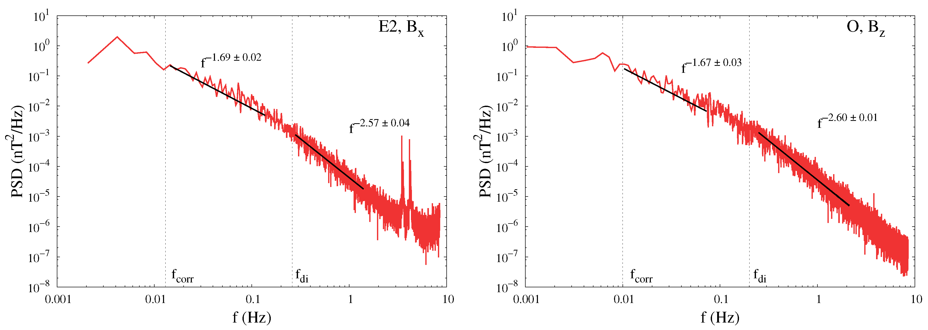
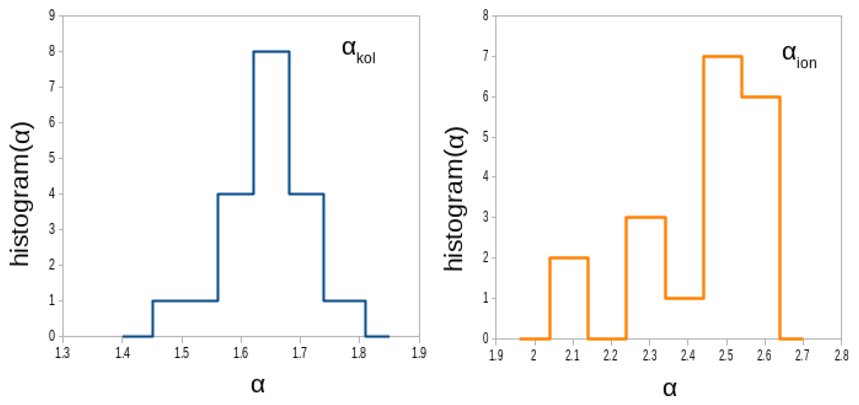
3.1. Magnetic Field Spectral Properties
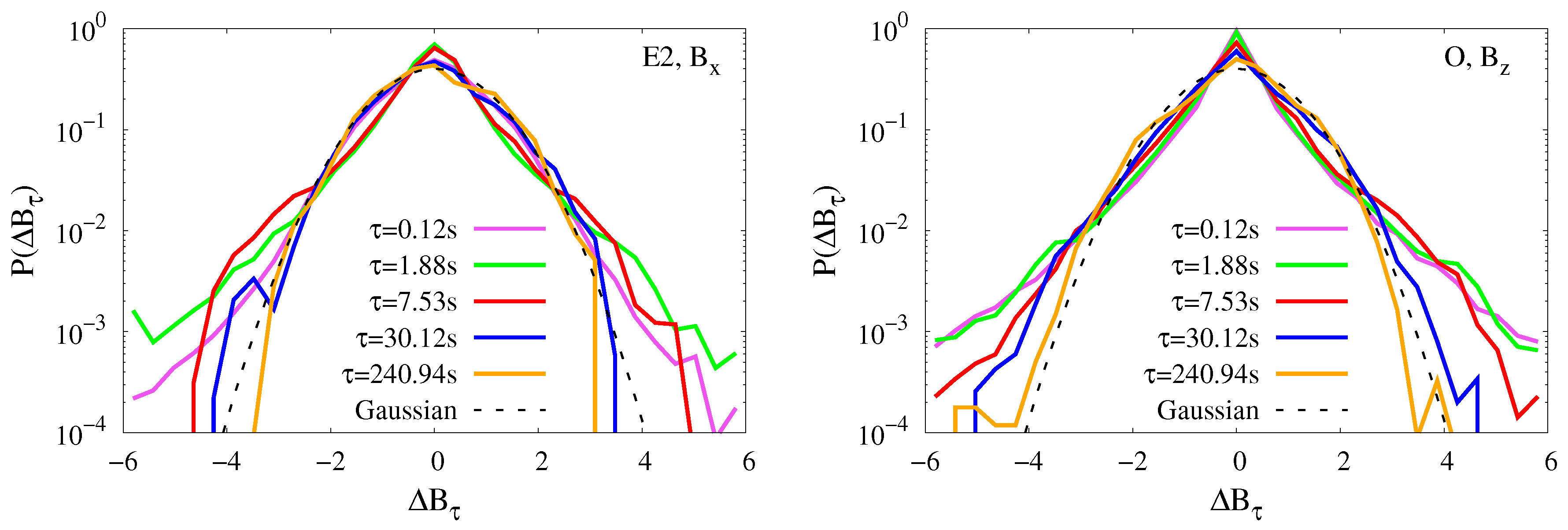
Figure 2 shows examples of the autocorrelation function versus time scale, for two different samples of the whole collection, one chosen among the mixed status (E2) and the other one among the weakly-mixed status (O). The behaviour of the autocorrelation function is typical of turbulent fields, i.e., with roughly parabolic shape near the origin, indicating the field smoothness in the “dissipative” range, followed by a slower decay to zero, indicative of the inertial range of turbulence [40]. For the example of Figure 2, the values of the time-scale at which the autocorrelation function approaches zero, are the following. Event E2: τ c o r r ( x ) = ( 33 ± 0.2 ) s , τ c o r r ( y ) = ( 23 ± 0.2 ) s , τ c o r r ( z ) = ( 30 ± 0.2 ) s ; Event O: τ c o r r ( x ) = ( 42 ± 0.2 ) s , τ c o r r ( y ) = ( 32 ± 0.2 ) s , τ c o r r ( z ) = ( 47 ± 0.2 ) s .
The values obtained for the three magnetic field components for all the intervals under study vary between 13 s and 58 s, in agreement with the typical values in this region [35,41].
The magnetic energy power spectra provide information about the scaling properties of the field fluctuations. Two examples are given in Figure 3 where we show two characteristic frequencies: the frequency related to the correlation time f c o r r = 1 / τ c o r r and the frequency f d i , related to the ion inertial length of a thermal ion d i = c / ω p i , i.e., the ratio between light speed and ion plasma frequency. The latter has been estimated assuming the validity of the argument given by Stawarz et al. [35].
Specifically, using the Taylor approximation of relation ω s c k · v ms and replacing the angular frequency ω with the spatial frequency f ω = 2 π f , we obtain 2 π f k v m s , and being the wave vector k = 1 / the inverse of a typical length (in this work, we use d i ), we have: 2 π f v m s d i f v m s 2 π d i . At large scales, the correlation frequency very well represents the large-scale boundary of the spectral inertial range. Similarly, the inertial range clearly breaks around the frequency associated with the ion inertial scale f d i , where kinetic plasma effects start being non-negligible, and in agreement with the usual observations of solar-wind and magnetosheath turbulence [42].
In the MHD range of scales, i.e., above the ion inertial length, the spectrum is well represented by a power law. We report even for the spectra, the measurements of the two selected events, E2 chosen among the mixed status and O for the weakly-mixed status. For the example, in the left panel of Figure 3, we obtain a scaling exponent 1.69 , while, for the right panel 1.67 . Both values are close to the Kolmogorov value 5 / 3 . The average exponent for the three magnetic field component PSDs for all the intervals is α k o l = 1.64 ± 0.08 , where the error is the standard deviation. Below the typical proton scales, the spectrum is compatible with a steeper power law with exponent which we find, for the examples presented in Figure 3, to be 2.57 for the B x component in sample E2, and 2.60 for the B z component in sample O. The exponents found for all components and all intervals lie in the range between 1.89 and 2.76 , with a mean value α i o n = 2.44 ± 0.19 .
The observed spectra seem to indicate that the typical behaviour of space plasma is retrieved in these samples, and that the turbulence might be developing as a consequence of, or superimposed to, the Kelvin–Helmholtz instability. Figure 4 shows how the spectral exponent α k o l and the exponent α i o n are distributed around the typical expected values.
The histograms, collecting the exponents for all magnetic components and for all events, show clearly that the inertial range exponent distribution is sharply peaked around the expected Kolmogorov value α k o l 5 / 3 . On the contrary, and in agreement with solar wind observations [43], the small-scale exponents are more broadly distributed around their mean α i o n 2.44 .

3.2. Intermittency

The statistical properties of turbulent fields cannot be fully described by spectra, and the intermittency in particular requires a more accurate statistical treatment of the fluctuations. For this reason, we have estimated the PDF for all components of the magnetic field increments at different scales, for all samples here considered. For each scale, the magnetic field increments were standardized by normalizing to their standard deviation to allow the comparison between the different scales. PDFs were thus computed as histograms normalized to the total number of field increments and to the equally spaced bin size, so that the integral of the whole PDF is one. Figure 5 shows two examples of the increment PDFs at five different scales, for the same two intervals and components already shown in previous figures. The black dashed line represents a reference Gaussian distribution. The probability distribution functions are characterized by the increasing deviation from Gaussian towards smaller scales [44,45,46], typical of intermittent turbulence. At small scales, the distributions show heavy tails indicating the presence of particularly intense magnetic field fluctuations, usually related to the presence of intermittent structures. Similar results were found for all intervals and for all magnetic field components.
A way to quantify the deviation from a Gaussian distribution is the normalized fourth-order moment of the increments, the kurtosis K. In all the intervals under study, the kurtosis of all magnetic field components has the typical Gaussian value K = 3 at large scales, roughly down to the correlation scale, and then increases toward small scales as a power law K ( l ) l κ . For all cases, the power-law fitting range was approximately located between the correlation time (at large time scales) and the time associated with the ion-inertial scale, via the Taylor hypothesis (at small time scale). This range is mostly consistent with the observed spectral inertial range, although in some occasions a small shift towards small scales is present. The scaling exponent κ gives a quantitative estimate of the intermittency, i.e., of the anomalous scaling of the magnetic fluctuations [47].
In Navier–Stokes turbulence, it is often observed that κ 0.1 [48]. In Figure 6, the scaling exponent of kurtosis is larger, consistent with a more efficient intermittency, for both datasets E2 and O.
Note that at small scales a saturation and decrease of the kurtosis is observed in about half of the cases, as shown in Figure 6 for the E2 event on the left side. For the other cases, the kurtosis keeps its increasing trend or shows a saturation (Figure 6 event O on the right side). The first behaviour, i.e., a saturation and decrease at small scales, is typical of the solar-wind magnetic fluctuations, while it was not usually observed in the magnetosheath (e.g., [35,49]). Although we can exclude instrumental noise effects (the observed scales are sufficiently far from the noise level, as also seen from the spectra), the reason for this behaviour is not fully understood, and it is outside of the scope of the present paper.

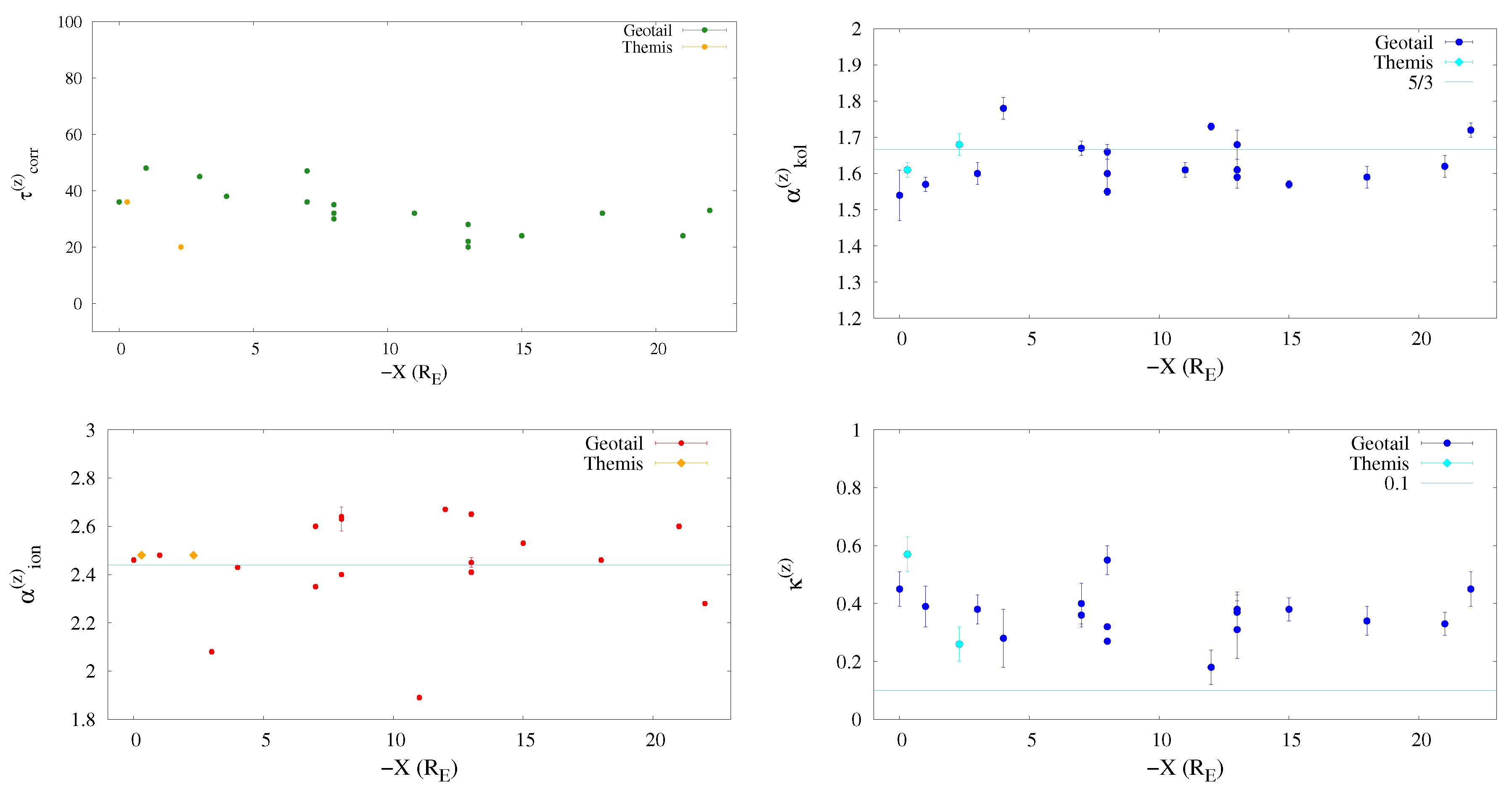
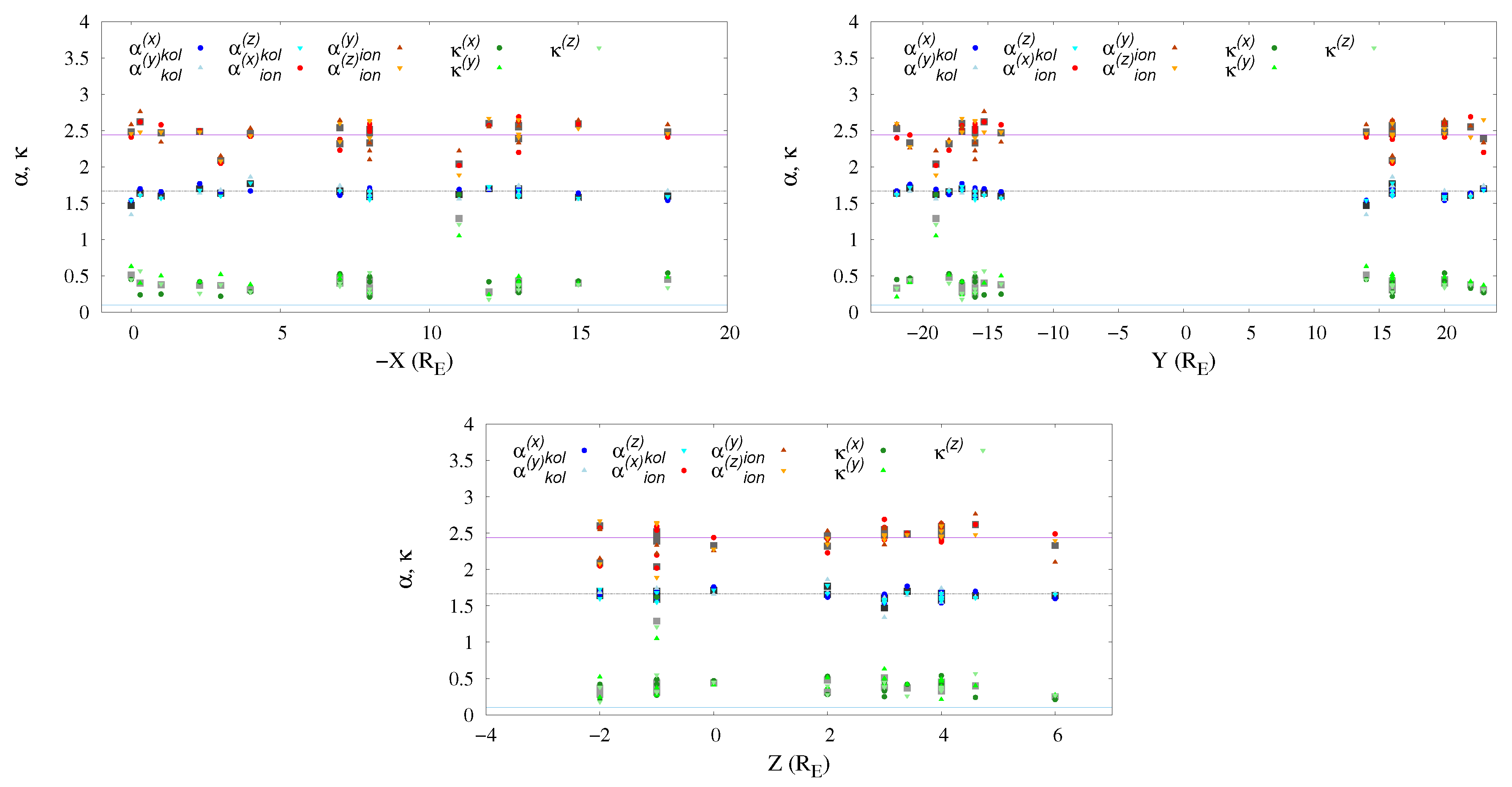
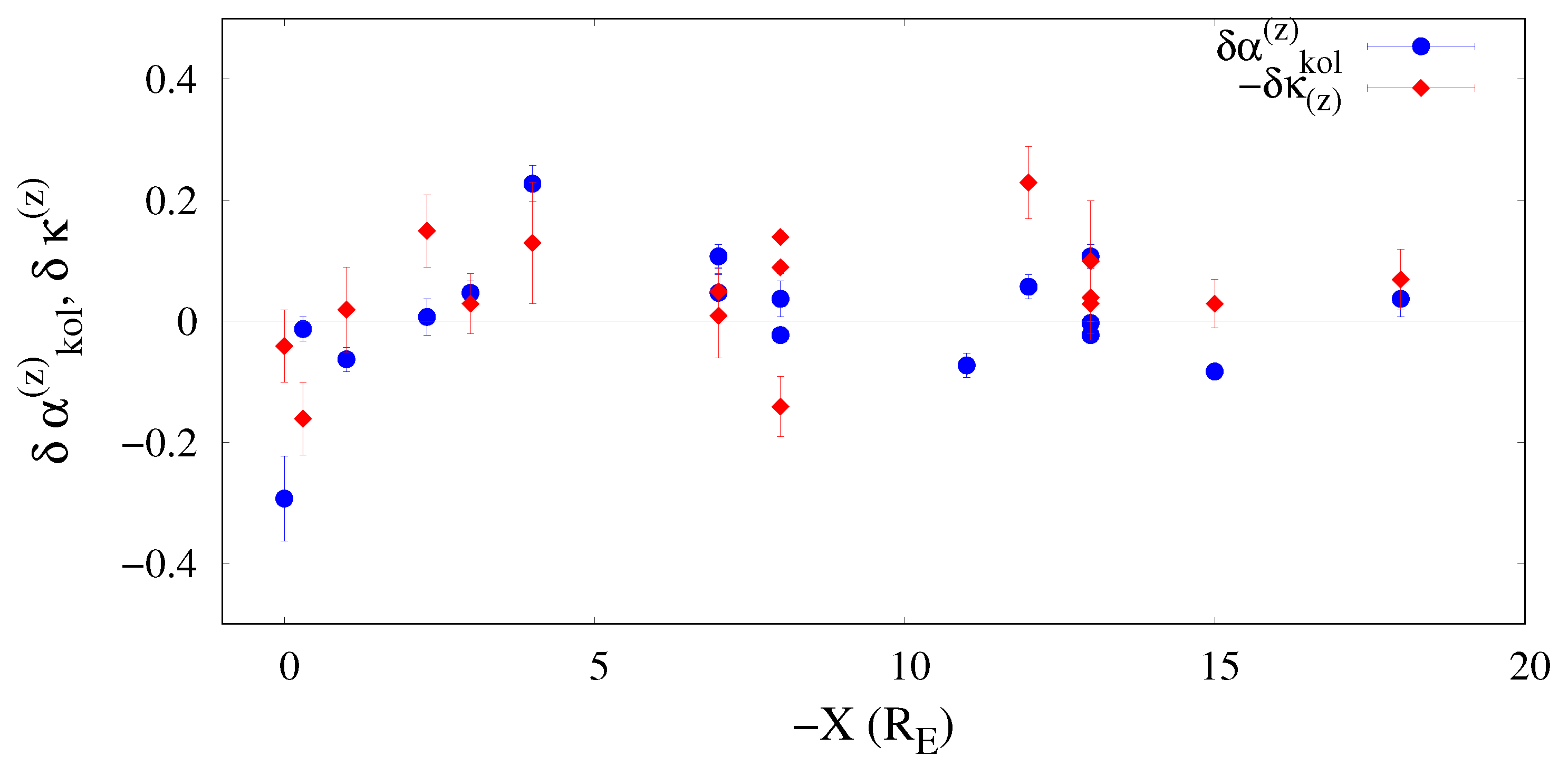
4. Evolution of the Turbulence along the Flank Magnetopause

Following the analysis of the properties of turbulence in each individual event, we now focus on the possibility to identify signatures of its evolution along the flank magnetopause by comparing the different samples under study. The position along the magnetopause likely corresponds to different stages of the KH evolution, whose possible influence on the turbulence characteristics will be discussed. Turbulence in the dayside magnetopause region is usually strong, and can have several sources besides the KHI [50,51]. These include for example magnetic reconnection poleward of the cusp [16,17,52,53,54,55,56], or kinetic Alfvén waves mode converted in the non-uniform magnetopause region from compressional fluctuations present in the dayside magnetosheath [36,37]. The turbulence observed in our sample could thus be either generated by the identified KHI, or pre-existent, due to other drivers, and modulated by the KHI.
We are interested in understanding if the statistical properties of the field fluctuations, which may be used as an indicator of the state of turbulence, evolve following the development of the KHI along the magnetopause. The majority of the intervals selected for this work were identified as collected in the mixing region of the KHI. This makes our database roughly homogeneous in terms of the macroscopic KHI geometry and of the spacecraft position within the instability structures in the shear direction (approximately corresponding to X in our reference frame). The upstream wind conditions were relatively similar for most of the intervals, as specified in Table A1 in Appendix A. Furthermore, all samples present comparable roll-up period of 2–4 minutes. Using the tailward flow speed listed in Table 1 to transform the period in wavelength, the resulting average KH wavelength is 6.4 R E , consistent with that reported in the literature [6,12,13,15,23]. In this approximation, the different intervals are thus samples of turbulence at different distances from the instability region, along KHI structures of comparable scale, allowing to study the modulation of turbulence caused by the instability.
Therefore, we will show the variation of the turbulence and intermittency parameters estimated in previous sections as a function of the spacecraft position in the magnetosheath. In Figure 7, the z-component magnetic field correlation scale τ (top left), the fitted spectral power-law index α k o l ( z ) of the z magnetic field component (in the Kolmogorov inertial range) (top right), the spectral index α i o n ( z ) (in the sub-ion range, i.e., for scales smaller than the typical ion scales) (bottom left), and the kurtosis scaling exponent κ are plotted as a function of the -X coordinate. The figure suggests a possible fluctuating behaviour of the parameters as the spacecraft position spans the X-coordinate, visible as a quasi-periodic modulation of the spectral exponents. Although such behaviour does not fit a periodic function, the approximate wavelength associated with such oscillation can be roughly estimated as 6 7 R E .
The amplitude of such modulation seems to decrease as the measurements are taken further away from the dusk-dawn line, and for X 15 R E the parameters seem to become more stabilized. Note that the fluctuations of the power-law index are typically larger than the estimated fitting error on each value (as clearly visible from the figures).
This result suggests that, for the observed KHI events, the vortex roll-up periodicity provides a modulation of the associated turbulence at all times, possibly due to the quasi-periodic alternation of dominating plasma (i.e., on both sides of the KHI interface) along the flanks. Eventually, turbulence converges towards a fully developed state, i.e., with a stabilized spectral index, after about 15 R E , where the two regions are finally mixed. Note that this type of evolution was also recently observed in numerical simulations of turbulence in the KHI [60].
This interpretation is corroborated by the fact that the observed modulation is persistent for most of the parameters obtained in this analysis. Indeed, the scaling exponent of kurtosis κ ( z ) , also shown in the bottom panel of Figure 7, also presents the same modulation, with similar periodicity. For a more comprehensive overview of our observation, the fitted power-law indexes α k o l , α i o n and the kurtosis scaling index κ are plotted together as a function of the -X, Y, Z coordinate (Figure 8), in order to better visualize the overall behavior which characterizes the KH vortices.
The spectral index α k o l at MHD scales is indicated by different shades of blue symbols for his three field components; similarly, α i o n is described by different red symbols for the three component, and the index κ of the kurtosis is indicated by green symbols. We have also plotted the mean of three component for each sample as grey squares. Moreover, reference lines at 5 / 3 , 2.44 and 0.101 are plotted for each exponent, respectively. The fluctuating behaviour is seen for all three indexes. This confirms the possible signature of transition to turbulence in the region downstream of the KH instability, with spectral and intermittency properties evolving while the KHI vortices roll-up. This interpretation requires the assumption that all KHI events studied here might be originated at the same distance from the dusk–dawn line, e.g., at magnetosphere nose, and that the development of the KHI under similar conditions is characterized by a similar evolution of turbulence.
It is noteworthy that the emergence of a clear anti-correlation between the κ and the two spectral indexes, although it is more evident between κ and α k o l . In order to look for correlations between the variations in the turbulence parameters, we directly compare the fluctuations around their means of the inertial range spectral exponent and of the kurtosis scaling exponent, as shown in Figure 9 as a function of -X for the z-component of the field. There is a hint of some correlation in the trend of the two indexes.
To quantitatively measure the amount of such correlations between all parameters, we computed the (linear) Pearson and (rank) Spearman correlation coefficients (respectively, C P and C S ) for all pairs of turbulent indexes. As also visualized in the scatter plots in Figure 10, the most correlated parameters are α k o l ( z ) and κ ( z ) (left panel at the top), α i o n ( z ) and κ ( z ) (right panel at the top), and the mean magnetosheath speed v m s vs κ (left bottom panel). The correlation timescale τ also is moderately correlated with the kurtosis scaling exponent for the z-component of the magnetic field (right bottom panel), while no significant correlation is observed with the other parameters. The presence of correlations, although moderate, strengthens the observation of the spatial structure along the KHI. The bulk plasma velocity correlation with the kurtosis scaling exponent could suggest a role of the velocity in modulating the turbulence. However, no correlation is observed with the spectral exponents, so that this possibility should be disregarded.

5. Conclusions

We have studied and characterized the properties of plasma turbulence and intermittency, along the tail-flank magnetopause and its boundary layer, when Kelvin–Helmholtz instability was reported. We have surveyed the Geotail and THEMIS data, recognized as rolled-up vortices by Fairfield et al. [12], Hasegawa et al. [15], Fairfield et al. [21], Fujimoto et al. [28], Stenuit et al. [29], Lin et al. [30], taken during satellite magnetopause crossings. Firstly, we have applied time-series analysis techniques to the collection of 20 samples, in order to obtain the autocorrelation function, the power spectrum, the probability distribution functions of the field increments and their kurtosis. The behaviour of the autocorrelation functions is standard, with values of the correlation scales τ c o r r that vary between 13 and 58 s, in agreement with typical values observed in this region. In the MHD range of scales, the spectrum is well represented by a power law with exponent 1.69 , not far from the Kolmogorov value 5 / 3 . Below the typical proton scales, the spectrum is instead compatible with a steeper power law with exponent which we find in the range between 1.89 and 2.76 , with a mean value α i o n = 2.44 . The inertial range clearly breaks around the frequency associated with the ion inertial scale f d i , where kinetic plasma effects start being non-negligible, and in agreement with the usual observation of solar-wind and magnetosheath turbulence [42]. Probability distribution functions are characterized by high tails and the deviation from Gaussian increases towards smaller scales [44,45,46]. The fat tails are due to particularly intense magnetic field fluctuations, usually related to the presence of structures. Finally, we have analysed the behaviour of the kurtosis. The range of scales where we showed the presence of a power-law is generally consistent with the spectral inertial range, and the scaling exponent κ gives a quantitative estimate of the intermittency [47]. In light of the results obtained, we have investigated the behaviour of several parameters as a function of the progressive departure along the Geocentric Solar Magnetosphere coordinates, which roughly represent the direction in which we expect the KHI vortices to evolve towards fully developed turbulence. It appears that a fluctuating behaviour of the parameters exist, visible as a decreasing, quasi-periodic modulation with an associated periodicity, estimated to correspond to approximately 6.4 R E . Such observed wavelength is consistent with the estimated vortices roll-up wavelength reported in the literature for these events [6,12,13,15,23]. The observed modulation seems robust, as it exists for most of the parameters considered in this analysis, which also present moderate correlations among each other. If the turbulence is pre-existent, it is possible that the KHI modulates its properties along the magnetosheath, as we observed.
On the other hand, if we assume that the KHI has been initiated near the magnetospheric nose and develops along the flanks, then the different intervals we study may be sampling the plasma at different stages of evolution of the KH-generated turbulence, after the instability has injected energy in a cascading process as large-scale structures.
Of course, a possible role of the KH boundaries (i.e., of the actual mixing conditions) cannot be excluded, although in that case more random fluctuations of the parameters would be expected. Instead, the presence of a modulation suggests that the KHI events are initiated at the nose, and their structure is relatively similar for all the events studied here. The initial injection scale is persistent as the scale of the modulation of the transition to turbulence. The evolving nature of turbulence is represented by the initially broad, then decreasing fluctuations of the spectral and intermittency indexes. Such regime could be associated with the transient competition between linear dynamics and the emergence of secondary instabilities, which later evolves to fully developed turbulence. In our sample, the observed parameters roughly converge to the typical values of fully developed turbulence at a distance 15 R E from the dusk–dawn line, corresponding to a factor of 2–3 in terms of the KHI vortex roll-up. This observation might be an indication of the typical distance for the observation of fully developed turbulence initiated by a KH instability. If this behaviour is general, it could be of relevance for KHI near interplanetary shocks, in the solar corona, and in the magnetotail, providing useful information for currently operating and future space missions, such as MMS, the Parker Solar Probe and Solar Orbiter.

Author Contributions

Conceptualization, F.D.M., A.R. and L.S.-V.; methodology, F.D.M., L.S.-V. and F.M.; software, F.D.M.; validation, F.D.M., L.S.-V., A.R. and H.H.; formal analysis, F.D.M. and L.S.-V.; investigation, F.D.M.; resources, A.R., F.M. and H.H.; data curation, F.D.M.; writing—original draft preparation, F.D.M., L.S.-V., and A.R.; writing—review and editing, F.D.M., L.S.-V., A.R., F.M. and H.H.

Funding

This research received no external funding.

Acknowledgments

Geotail magnetic field and plasma data were provided by T. Nagai (H. Hayakawa and/or Y. Saito) through DARTS at Institute of Space and Astronautical Science, JAXA in Japan. L.S.-V. and A.R. acknowledge support from the Consiglio Nazionale delle Ricerche (CNR) Short Term Mobility program 2014, and from the MCF Visiting Professor programme 2014–2015 of Université Paris Sud.

Conflicts of Interest

The authors declare no conflict of interest. The funders had no role in the design of the study; in the collection, analyses, or interpretation of data; in the writing of the manuscript, or in the decision to publish the results.

Appendix A. Additional Information about Daily Conditions of the Upstream Solar Wind

By using the OMNI database provided by NASA (see the internet address https://omniweb.gsfc.nasa.gov), we have checked the solar wind (SW) conditions relative to the intervals used for each event described. The daily conditions are listed in Table A1, collecting the magnetic field magnitude | B s w | and components, the average values of bulk speed | V s w | and velocity components, the density n s w and temperature T s w . Conditions are generally similar in terms of bulk speed, with some differences in field magnitude and temperature. However, we have checked that these are basically uncorrelated with the turbulence parameters, with correlation coefficients 0.1 .
Table A1. Event List of rolled-up vortices detected by Geotail over nine years from 1995 to 2003, adapted from Hasegawa et al. [15]. The last two events were detected by THEMIS probe C, adapted by Lin et al. [30]. We collected the daily conditions of solar wind: the magnetic field magnitude | B s w | , the mean values of three components of the field B x s w , B y s w , B z s w , the average values of bulk speed | V s w | , the mean values of three components of the velocity V x s w , V y s w , V z s w , the values of the proton density n s w and proton temperature T s w .
Geotail Mission
EventInterval
(UT)
| B sw |
(nT)
B x sw , B y sw , B z sw
(nT)
| V sw |
(km/s)
V x sw , V y sw , V z sw
(km/s)
n sw
(1/cm3)
T sw
(K)
S1995-03-24 0600-08009.71.4; −4.5; 8.3332−332; 12.3; −6,318.118,018
O1997-01-10 2050-240013.7−2.5; −11.8; 5.7414−414; 3.4; −13.920.611,343
P1997-01-11 0400-050022.2−7.5; −3.8; 20.3454−453; −19.0; 16.014.1116,348
Q1997-02-12 1430-16003.5−0.7; −0.3; 3.3382−382; −4.1; −2.55.422,156
T1998-04-13 0315-04308.84.5; −2.9; 6.7390−390; −5.5; 4.83.823,776
L1998-08-01 0530-07309.7−2.6; 7.8; 8.9404−404; −7.9; −8.28.335,023
D1998-12-27 1800-21005.2−1.8; 6.2; 4.7371−370; −10.1; −29.34.434,764
N1999-02-15 1445-15158.2−2.0; 3.9; 5.2600−599; 25.5; −8.03.7187,717
M1999-07-20 0630-07306.3−2.1; 0.2; 5.9303−303; 3.2; −5.015.425,486
E2000-11-01 1030-12006.64.5; −0.2; 4.5443−443; −8.7; −11.66.286,515
H2001-01-25 1330-16303.41.5; −1.7; 1.8372−372; 10.4; −13.14.510,762
B2001-11-16 1900-20008.9−3.6; 5.4; 2.9379−378; 1.6; −14.54.059,474
C2001-12-07 2000-21305.42.3; −2.0; 3.4462−461; 19.3; 9.13.1101,406
E22002-03-25 0530-090017.05.7; −13.1; 9.0444−443; 6.5; 17.95.737,541
F2002-03-25 1000-130014.85.2; −11.0; 8.2435−435; −9.2; 12.16.720,890
A2002-10-15 2100-230014.92.7; 8.6; 5.5532−525; 49.8; −61.14.1812,629
R2003-07-17 0330-05003.92.7; −1.3; 1.8632−632; 11.5; 13.52.6190,142
THEMIS Mission
TH12008-11-06 0850-09202.72.1; −0.8; 1.5288−288; −8.7; 3.16.514,542
TH22008-11-18 0720-07303.4-0.9; −1.1; 3.1347−346; −15.1; 9.94.531,423

References

  1. Pucci, F.; Malara, F.; Perri, S.; Zimbardo, G.; Sorriso-Valvo, L.; Valentini, F. Energetic particle transport in the presence of magnetic turbulence: influence of spectral extension and intermittency. Mon. Not. R. Astron. Soc. 2016, 459, 3395–3406. [Google Scholar] [CrossRef]
  2. Zimbardo, G.; Greco, A.; Veltri, P.; Voros, Z.; Taktakishvili, A.L. Magnetic turbulence in and around the Earth’s magnetosphere. Astrophys. Space Sci. Trans. 2008, 4, 35–40. [Google Scholar] [CrossRef]
  3. Mitchell, D.G.; Kutchko, F.; Williams, D.J.; Eastman, T.E.; Frank, L.A.; Russell, C.T. An extended study of the low-latitude boundary layer on the dawn and dusk flanks of the magnetosphere. J. Geophys. Res. 1987, 92, 7394–7404. [Google Scholar] [CrossRef]
  4. Bavassano Cattaneo, M.B.; Marcucci, M.F.; Bogdanova, Y.V.; Réme, H.; Dandouras, I.; Kistler, L.M.; Lucek, E. Global reconnection topology as inferred from plasma observations inside Kelvin–Helmholtz vortices. Ann. Geophys. 2010, 28, 893–906. [Google Scholar] [CrossRef]
  5. Johnson, J.R.; Wing, S.; Delamere, P.A. Kelvin Helmholtz Instability in Planetary Magnetospheres. Space Sci. Rev. 2014, 184, 1–31. [Google Scholar] [CrossRef]
  6. Hasegawa, H. Comment on "Evolution of Kelvin–Helmholtz activity on the dusk flank magnetopause" by Foullon et al. J. Geophys. Res. 2009, 114, A03205. [Google Scholar] [CrossRef]
  7. Sckopke, N.; Paschmann, G.; Haerendel, G.; Sonnerup, B.U.; Bame, S.J.; Forbes, T.G.; Hones, E.W.; Russell, C.T. Structure of the low-latitude boundary layer. J. Geophys. Res. 1981, 86, 2099–2110. [Google Scholar] [CrossRef]
  8. Sonnerup, B. Theory of the low-latitude boundary layer. J. Geophys. Res. 1980, 85, 2017–2026. [Google Scholar] [CrossRef]
  9. Lui, A.T.Y.; Venkatesan, D.; Murphree, J.S. Auroral bright spots on the dayside oval. J. Geophys. Res. 1989, 94, 5515. [Google Scholar] [CrossRef]
  10. Yamamoto, T. A linear analysis of the hybrid Kelvin-Helmholtz/Rayleigh-Taylor instability in an electrostatic magnetosphere-ionosphere coupling system. J. Geophys. Res. 2008, 113, A06206. [Google Scholar] [CrossRef]
  11. Chen, S.H.; Kivelson, M.G. On nonsinusoidal waves at the Earth’s magnetopause. Geophys. Res. Lett. 1993, 20, 2699–2702. [Google Scholar] [CrossRef]
  12. Fairfield, D.H.; Otto, A.; Mukai, T.; Kokubun, S.; Lepping, R.P.; Steinberg, J.T.; Lazarus, A.J.; Yamamoto, T. Geotail observations of the Kelvin–Helmholtz instability at the equatorial magnetotail boundary for parallel northward fields. J. Geophys. Res. 2000, 105, 21159–21173. [Google Scholar] [CrossRef]
  13. Kivelson, M.G.; Chen, S.H. The Magnetopause: Surface Waves and Instabilities and Their Possible Dynamical Consequences; Geophys. Monogr. Ser., 90; Song, P., Sonnerup, B.U.Ö., Thomsen, M.F., Eds.; American Geophysicsl Union: Washington, DC, USA, 1995; Volume 20, pp. 257–268. [Google Scholar]
  14. Fujimoto, M.; Tonooka, T.; Mukai, T. Vortex-Like Fluctuations in the Magnetotail Flanks and Their Possible Roles in Plasma Transport; Geophys. Monogr. Ser. 133; Newell, P.T., Onsager, T., Eds.; American Geophysicsl Union: Washington, DC, USA, 2003; pp. 241–251. [Google Scholar]
  15. Hasegawa, H.; Fujimoto, M.; Takagi, K.; Saito, Y.; Mukai, T.; Réme, H. Single-spacecraft detection of rolled-up Kelvin–Helmholtz vortices at the flank magnetopause. J. Geophys. Res. 2006, 111, A09203. [Google Scholar]
  16. Terasawa, T.; Fujimoto, M.; Mukai, T.; Shinohara, I.; Saito, Y.; Yamamoto, T.; Machida, S.; Kokubun, S.; Lazarus, A.J.; Steinberg, J.T.; et al. Solar wind control of density and temperature in the near-Earth plasma sheet: Wind/Geotail collaboration. Geophys. Res. Lett. 1997, 24, 935–938. [Google Scholar] [CrossRef]
  17. Wing, S.; Newell, P.T. 2D plasma sheet ion density and temperature profiles for northward and southward IMF. Geophys. Res. Lett. 2002, 29, 9. [Google Scholar] [CrossRef]
  18. Sundberg, T.; Boardsen, S.A.; Slavin, J.A.; Anderson, B.J.; Korth, H.; Zurbuchen, T.H.; Raines, J.M.; Solomon, S.C. MESSENGER orbital observations of large-amplitude Kelvin-Helmholtz waves at Mercury’s magnetopause. J. Geophys. Res. 2012, 117, A04216. [Google Scholar] [CrossRef]
  19. Nakamura, T.K.M.; Hasegawa, H.; Daughton, W.; Eriksson, S.; Li, W.Y.; Nakamura, R. Turbulent mass transfer caused by vortex induced reconnection in collisionless magnetospheric plasmas. Nat. Commun. 2017, 8, 1582. [Google Scholar] [CrossRef] [PubMed]
  20. Chen, S.H.; Kivelson, M.G.; Gosling, J.T.; Walker, R.J.; Lazarus, A.J. Anomalous aspects of magnetosheath flow and of the shape and oscillations of the magnetopause during an interval of strongly northward interplanetary magnetic field. J. Geophys. Res. 1993, 98, 5727–5742. [Google Scholar] [CrossRef] [Green Version]
  21. Fairfield, D.H.; Kuznetsova, M.M.; Mukai, T.; Nagai, T.; Gombosi, T.I.; Ridley, A.J. Waves on the dusk flank boundary layer during very northward interplanetary magnetic field conditions: Observations and simulation. J. Geophys. Res. 2007, 112, A08206. [Google Scholar] [CrossRef]
  22. Farrugia, C.J.; Gratton, F.T.; Torbert, R.B. Viscous-type processes in the solar wind-magnetosphere interaction. Space Sci. Rev. 2001, 95, 443–456. [Google Scholar]
  23. Hasegawa, H.; Fujimoto, M.; Phan, T.D.; Réme, H.; Balogh, A.; Dunlop, M.W.; Hashimoto, C.; Tandokoro, R. Transport of solar wind into Earth’s magnetosphere through rolled-up Kelvin–Helmholtz vortices. Nature 2004, 430, 755–758. [Google Scholar] [CrossRef] [PubMed]
  24. Kokubun, S.; Yamamoto, T.; Acuna, M.H.; Hayashi, K.; Shiokawa, K.; Kawano, H. The GEOTAIL magnetic field experiment. J. Geomag. Geo-Electr. 1994, 46, 7–21. [Google Scholar] [CrossRef]
  25. Otto, A.; Fairfield, D.H. Kelvin-Helmholtz instability at the magnetotail boundary: MHD simulation and comparison with Geotail observations. J. Geophys. Res. 2000, 105, 17521. [Google Scholar] [CrossRef]
  26. Foullon, C.; Farrugia, C.J.; Fazakerley, A.N.; Owen, C.J.; Gratton, F.T.; Torbert, R.B. Evolution of Kelvin-Helmholtz activity on the dusk flank magnetopause. J. Geophys. Res. 2008, 113, A11203. [Google Scholar] [CrossRef]
  27. Fairfield, D.H.; Farrugia, C.J.; Mukai, T.; Nagai, T.; Federov, A. Motion of the dusk flank boundary layer caused by solar wind pressure changes and the Kelvin-Helmholtz instability: 10–11 January 1997. J. Geophys. Res. 2003, 108, 1460–1471. [Google Scholar] [CrossRef]
  28. Fujimoto, M.; Terasawa, T.; Mukai, T. The Low-Latitude Boundary Layer in the Tail-Flanks; Geophysical Monograph 105; Nishida, A., Baker, D.N., Cowley, S.W.H., Eds.; American Geophysical Union: Washington, DC, USA, 1998; pp. 33–44. [Google Scholar]
  29. Stenuit, H.; Fujimoto, M.; Fuselier, S.A.; Sauvaud, J.A.; Wing, S.; Fedorov, A.; Budnik, E.; Savin, S.P.; Trattner, K.J.; Angelopoulos, V.; et al. Multispacecraft study on the dynamics of the dusk-flankmagnetosphere under northward IMF: 10–11 January 1997. J. Geophys. Res. 2002, 107, 1333. [Google Scholar] [CrossRef]
  30. Lin, D.; Wang, C.; Li, W.; Tang, B.; Guo, X.; Peng, Z. Properties of Kelvin–Helmholtz waves at the magnetopause under northward interplanetary magnetic field: Statistical study. J. Geophys. Res. 2014, 119, 7485–7494. [Google Scholar] [CrossRef]
  31. Takagi, K.; Hashimoto, C.; Hasegawa, H.; Fujimoto, M.; TanDokoro, R. Kelvin-Helmholtz instability in a magnetotail flank-like geometry: Three-dimensional MHD simulations. J. Geophys. Res. 2006, 111, A08202. [Google Scholar] [CrossRef]
  32. Taylor, G.I. The Spectrum of Turbulence. Proc. R. Soc. Lond. A 1938, 164, 476–490. [Google Scholar] [CrossRef] [Green Version]
  33. Klein, K.G.; Howes, G.G.; TenBarge, J.M. The violation of the Taylor hypothesis in measurements of solar wind turbulence. Astrophys. J. Lett. 2014, 790, L20. [Google Scholar] [CrossRef]
  34. Fredricks, R.W.; Coroniti, F.V. Ambiguities in the deduction of rest frame fluctuation spectra from spectra computed in moving frames. J. Geophys. Res. 1976, 81, 5591–5595. [Google Scholar] [CrossRef]
  35. Stawarz, J.E.; Eriksson, S.; Wilder, F.D.; Ergun, R.E.; Schwartz, S.J.; Pouquet, A.; Burch, J.L.; Giles, B.L.; Khotyaintsev, Y.; Contel, O.L.; et al. Observations of turbulence in a Kelvin–Helmholtz event on 8 September 2015 by the Magnetospheric Multiscale mission. J. Geophys. Res. 2016, 121, 11021–11034. [Google Scholar] [CrossRef]
  36. Chaston, C.C.; Wilber, M.; Mozer, F.S.; Fujimoto, M.; Goldstein, M.L.; Acuna, M.; Réme, H.; Fazakerley, A. Mode Conversion and Anomalous Transport in Kelvin–Helmholtz Vortices and Kinetic Alfvén Waves at the Earth’s Magnetopause. Phys. Rev. Lett. 2007, 99, 175004. [Google Scholar] [CrossRef] [PubMed]
  37. Chaston, C.C.; Bonnell, J.W.; Clausen, L.; Angelopoulos, V. Energy transport by kinetic-scale electromagnetic waves in fast plasma sheet flows. J. Geophys. Res. 2012, 117, A09202. [Google Scholar] [CrossRef]
  38. Hapgood, M.A. Space physics coordinate transformations-A user guide. Planet Space Sci. 1992, 40, 711–717. [Google Scholar] [CrossRef]
  39. Russell, C.T. Geophysical Coordinate Transformations. Cosmic Electrodyn. 1971, 2, 184–196. [Google Scholar]
  40. Pope, S. Turbulent Flows; Cambridge University Press: Cambridge, UK, 2000. [Google Scholar]
  41. Gutynska, O.; Šafránková, J.; Němeček, Z. Correlation length of magnetosheath fluctuations: Cluster statistics. Ann. Geophys. 2008, 26, 2503–2513. [Google Scholar] [CrossRef] [Green Version]
  42. Leamon, R.J.; Smith, C.W.; Ness, N.F.; Matthaeus, W.H.; Wong, H.K. Observational constraints on the dynamics of the interplanetary magnetic field dissipation range. J. Geophys. Res. 1998, 103, 4775–4787. [Google Scholar] [CrossRef]
  43. Sahraoui, F.; Belmont, G.; Rezeau, L.; Cornilleau-Wehrlin, N.; Pinçon, J.L.; Balogh, A. Anisotropic Turbulent Spectra in the Terrestrial Magnetosheath as Seen by the Cluster Spacecraft. Phys. Rev. Lett. 2006, 96, 075002. [Google Scholar] [CrossRef]
  44. Frisch, U. Turbulence. The Legacy of A. N. Kolmogorov; Cambridge University Press: Cambridge, UK, 1995. [Google Scholar]
  45. Sorriso-Valvo, L.; Carbone, V.; Veltri, P.; Consolini, G.; Bruno, R. Intermittency in the solar wind turbulence through probability distribution functions of fluctuations. Geophys. Res. Lett. 1999, 26, 1801–1804. [Google Scholar] [CrossRef] [Green Version]
  46. Bruno, R.; Carbone, V. The Solar Wind as a Turbulence Laboratory. Living Rev. Sol. Phys. 2005, 2, 4. [Google Scholar] [CrossRef]
  47. Sreenivasan, K.R.; Antonia, R.A. The phenomenology of small-scale turbulence. Ann. Rev. Fluid Mech. 1997, 29, 435–472. [Google Scholar] [CrossRef]
  48. Anselmet, F.; Gagne, Y.; Hopfinger, E.J.; Antonia, R.A. High-order velocity structure functions in turbulent shear flows. J. Fluid Mech. 1984, 140, 63–89. [Google Scholar] [CrossRef]
  49. Chhiber, R.; Chasapis, A.; Bandyopadhyay, R.; Parashar, T.N.; Matthaeus, W.H.; Maruca, B.A.; Moore, T.E.; Burch, J.L.; Torbert, R.B.; Russell, C.T.; et al. Higher-order turbulence statistics in the Earth’s magnetosheath and the solar wind using Magnetospheric Multiscale observations. J. Geophys. Res. 2018, 123, 9941–9954. [Google Scholar] [CrossRef]
  50. Book, D.L.; Sibeck, D.G. Plasma transport through the magnetopause turbulent interchange processes. J. Geophys. Res. 1995, 100, 9567–9573. [Google Scholar] [CrossRef]
  51. Labelle, J.; Treumann, R.A. Plasma waves at the dayside magnetopause. Space Sci. Rev. 1988, 47, 175–202. [Google Scholar] [CrossRef]
  52. Bavassano Cattaneo, M.B.; Marcucci, M.F.; Retinò, A.; Pallocchia, G.; Réme, H.; Dandouras, I.; Kistler, L.M.; Klecker, B.; Carlson, C.W.; Korth, A.; et al. Kinetic signatures during a quasi-continuous lobe reconnection event: Cluster Ion Spectrometer (CIS) observations. J. Geophys. Res. 2006, 111, A09212. [Google Scholar] [CrossRef]
  53. Frey, H.U.; Phan, T.D.; Fuselier, S.A.; Mende, S.B. Continuous magnetic reconnection at Earth’s magnetopause. Nature 2003, 426, 533–537. [Google Scholar] [CrossRef]
  54. Phan, T.D.; Dunlop, M.W.; Paschmann, G.; Klecker, B.; Bosqued, J.M.; Réme, H.; Balogh, A.; Twitty, C.; Mozer, F.S.; Carlson, C.W.; et al. Cluster observations of continuous reconnection at the magnetopause under steady interplanetary magnetic field conditions. Ann. Geophys. 2004, 22, 2355–2367. [Google Scholar] [CrossRef] [Green Version]
  55. Retinò, A.; Bavassano Cattaneo, M.B.; Marcucci, M.F.; Vaivads, A.; André, M.; Khotyaintsev, Y.; Phan, T.; Pallocchia, G.; Réme, H.; Möbius, E.; et al. Cluster multispacecraft observations at the high-latitude duskside magnetopause: Implications for continuous and component magnetic reconnection. Ann. Geophys. 2005, 23, 461–473. [Google Scholar]
  56. Song, P.; Russell, C.T. A model of the formation of the low-latitude boundary layer. J. Geophys. Res. 1992, 97, 1411. [Google Scholar] [CrossRef]
  57. Breuillard, H.; Yordanova, E.; Vaivads, A.; Alexandrova, O. The effects of kinetic instabilities on small-scale turbulence in Earth’s magnetosheath. Astrophys. J. 2016, 829, 54–60. [Google Scholar] [CrossRef]
  58. Zimbardo, G.; Greco, A.; Sorriso-Valvo, L.; Perri, S.; Vöros, Z.; Aburjania, G.; Chargazia, K.; Alexandrova, O. Magnetic turbulence in the geospace environment. Space Sci. Rev. 2010, 156, 89–134. [Google Scholar] [CrossRef]
  59. Alexandrova, O.; Chen, C.H.K.; Sorriso-Valvo, L.; Horbury, T.S.; Bale, S.D. Solar Wind Turbulence and the Role of Ion Instabilities. Space Sci. Rev. 2013, 178, 101–139. [Google Scholar] [CrossRef] [Green Version]
  60. Rossi, C.; Califano, F.; Retinò, A.; Sorriso-Valvo, L.; Henri, P.; Servidio, S.; Valentini, F.; Chasapis, A.; Rezeau, L. Two-fluid numerical simulations of turbulence inside Kelvin–Helmholtz vortices: Intermittency and reconnecting current sheets. Phys. Plasmas 2015, 22, 122303. [Google Scholar] [CrossRef]
Figure 1. Locations of rolled-up Kelvin–Helmholtz events identified from Geotail (light-blue/blue dot) and THEMIS (red diamond).
Atmosphere 10 00561 g001
Figure 2. The autocorrelation function for three component of magnetic field, related to the event E2 in the left panel and the event O at the right.
Atmosphere 10 00561 g002
Figure 3. Two examples of the one-dimensional power spectral density (PSD) of the magnetic field. We show here the PSD of B x for the dataset E2 (left panel) and of B z for the dataset O (right panel). A Kolmogorov-like spectrum is observed at the MHD scale, while a steeper power law is suggested below ion scales. The vertical black dashed lines indicate the frequency f d i related to the ion inertial length d i , and the frequency related to the correlation time f c o r r .
Atmosphere 10 00561 g003
Figure 4. Histograms of the total number of events with the spectral exponent α k o l , distributed around the Kolmogorov value 5/3 and the exponent α i o n , distributed around the value 2.44 . The exponents refer to all three components of the field.
Atmosphere 10 00561 g004
Figure 5. Probability distribution functions of the normalized increments Δ B τ ( x ) are shown in the left panel for sample E2 and in the right panel for sample O. The black dashed line is a Gaussian distribution used as reference.
Atmosphere 10 00561 g005
Figure 6. The scaling dependence of the kurtosis K for two samples, E2 on the left and O on the right. The Gaussian value K = 3 is indicated, as well as power-law fit in the inertial range for the two cases. The vertical black dashed lines indicate the inertial period τ d i related to the frequency f d i , and the correlation time τ c o r r .
Atmosphere 10 00561 g006
Figure 7. The correlation scale of the component B z (left-top panel), the fitted power-law index (component z of magnetic field), at MHD scales (right-top panel) and below ion scale of energy spectra (left-bottom panel), as a function of -X coordinate. The value expected for a Kolmogorov-like spectrum is –5/3 that corresponds to the horizontal green line in the top panel. The small-scale reference value is 2.44 [43,57,58,59]. A modulation is suggested, during the departure along -X coordinate, consistently because the error that affect measures are significantly smaller than the α -index values. In the right-bottom panel, the fitted power-law index of the kurtosis is plotted as a function of -X coordinate. The reference value is κ = 0.101 , which is typical value observed in Navier–Stokes turbulence [48].
Atmosphere 10 00561 g007
Figure 8. All fitted power-law index, i.e., α k o l m at MHD scales (blue symbols), α i o n at ion scales (red symbols) and κ scaling exponent of the kurtosis (green symbols), as a function of -X, Y, Z coordinate. Different shades of color and symbol shape refer to the different component (see legend). The mean value of each sample is reported as grey or black square. The overall fluctuating behaviour is seen for all three indexes.
Atmosphere 10 00561 g008
Figure 9. The fluctuation of the fitted power-law index for component z of energy spectra at MHD scales, i.e., α k o l m (blue dots) and the fluctuation of the power-law index for component z of the scaling exponent κ of the kurtosis (red dots) as a function of -X coordinate.
Atmosphere 10 00561 g009
Figure 10. Top left panel: the z-component of the scaling exponent κ as a function of the same component of the scaling exponent α k o l . Top right panel: the z-component of the scaling exponent κ as a function of the same component of the scaling exponent α i o n . Bottom left panel: the x-component of the scaling exponent κ as a function of the same component of the velocity field. Bottom right panel: the z-component of the scaling exponent κ as a function of the magnetic field correlation timescale τ . For each pair of parameters, the largest correlation coefficients, Pearson’s ( C P ) or Spearman’s ( C S ), is indicated in the corresponding panel.
Atmosphere 10 00561 g010
Table 1. Event List of rolled-up vortices detected by Geotail over nine years from 1995 to 2003, adapted from Hasegawa et al. [15]. The last two events were detected by THEMIS probe C, adapted by Lin et al. [30].
GEOTAIL MISSION
EventIntervalGSM PositionIMF ConditionMixing StatusPeriod v ms λ
S1995-03-24 0600-0800(−15, 20, 4)ES1 NBZ2Mixed2–32275.3
O1997-01-10 2050-2400(−7, 16, 4)ND3 NBZ after N-t4Weakly mixed2–31694.0
P1997-01-11 0400-0500(−13, 16, 4)ES NBZMixed∼ 32196.2
Q1997-02-12 1430-1600(−13, 22, 3)ES NBZMixed∼ 22815.3
T1998-04-13 0315-0430(−18, 20, 4)ES NBZMixed2–33127.3
L1998-08-01 0530-0730( 0, 14, −3)ES NBZMixed∼ 3922.6
D1998-12-27 1800-2100(−21, −22, −4)ES NBZMixed3–42478.1
N1999-02-15 1445-1515( −4, 16, 2)NBZ after N-tMixed∼ 22795.3
M1999-07-20 0630-0730( −3, 16, −2)ES NBZMixed2–32305.4
E2000-11-01 1030-1200( −8, −16, 6)ES NBZMixed2-32987.0
H2001-01-25 1330-1630(−22, −21, 0)ES NBZMixed∼ 51828.6
B2001-11-16 1900-2000(−7, −18, 2)Extended NBZ (often ND)Weakly mixed2–31834.3
C2001-12-07 2000-2130(−11, −19, −1)SNBZ5 after N-tWeakly mixed∼ 32577.3
E22002-03-25 0530-0900(−12, −17, −2)ES NBZMixed2–32997.0
F2002-03-25 1000-1300(−8, −16, −1)ES NBZMixed2–3299, 3477.0, 8.2
A2002-10-15 2100-2300(−1, −14, 3)Extended NBZMixed2–33327.8
R2003-07-17 0330-0500(−13, 23, −1)ND NBZ after N-tWeakly mixed∼ 24197.9
THEMIS MISSION
TH12008-11-06 0850-0920(−0.3, −15.3, 4.6)ES NBZMixed∼ 22883.3
TH22008-11-18 0720-0730(−2.3, −17, 3.4)ES NBZMixed∼ 33483.5
E S 1 : extended strong; N B Z 2 : northward IMF; N D 3 : non dominant; N t 4 : N-turning; S N B Z 5 : strong NBZ; Mixed/Weakly mixed means that a significant/small amount of magnetosheath ions was identified, i.e., n>/</1/cm3, in the BL.
Table 2. Values of the magnetosheath mean bulk velocity v m s , the Alfvén speed v A and the angle α between B 0 and v m s estimated for each interval.
v A (km/s) v ms (km/s) α (deg)
A547332104,34
B31518380,83
C345257117,32
D20424768,41
E26829899,1
E240029960,69
F34434776,15
H18218265,2
L2869272,58
M20023092,84
N23427985,41
O23216971,98
P26821964,57
Q18128190,8
R260419110,54
S17322799,84
T45631255,97
TH121928872,76
TH2307348139,23

