Added Value of Atmosphere-Ocean Coupling in a Century-Long Regional Climate Simulation


Abstract
:1. Introduction
- How sensitive is the atmosphere, namely the precipitation and 2 m temperature, to SST changes in the model system?
- Does the interactive coupling of atmosphere and ocean have an effect over the continental areas?
- Is there any large-scale added skill in the precipitation and in the 2 m temperature variables in the coupled simulation compared to the uncoupled one?
2. Data
2.1. Uncoupled Simulation
2.2. Coupled Simulation
2.3. Observations
3. Methods
3.1. Sensitivity Studies
3.2. Mean Square Error Skill Score
4. Results
4.1. Sensitivity of CCLM to SST
4.2. Precipitation
4.3. 2 m Temperature
5. Discussion and Conclusions
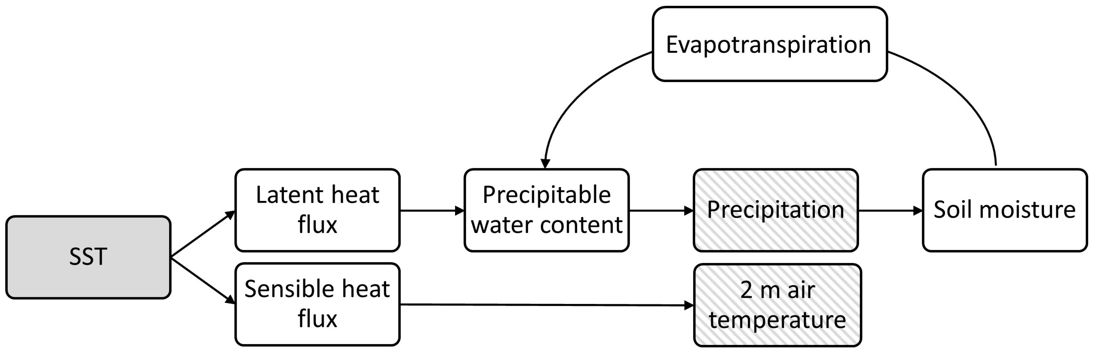
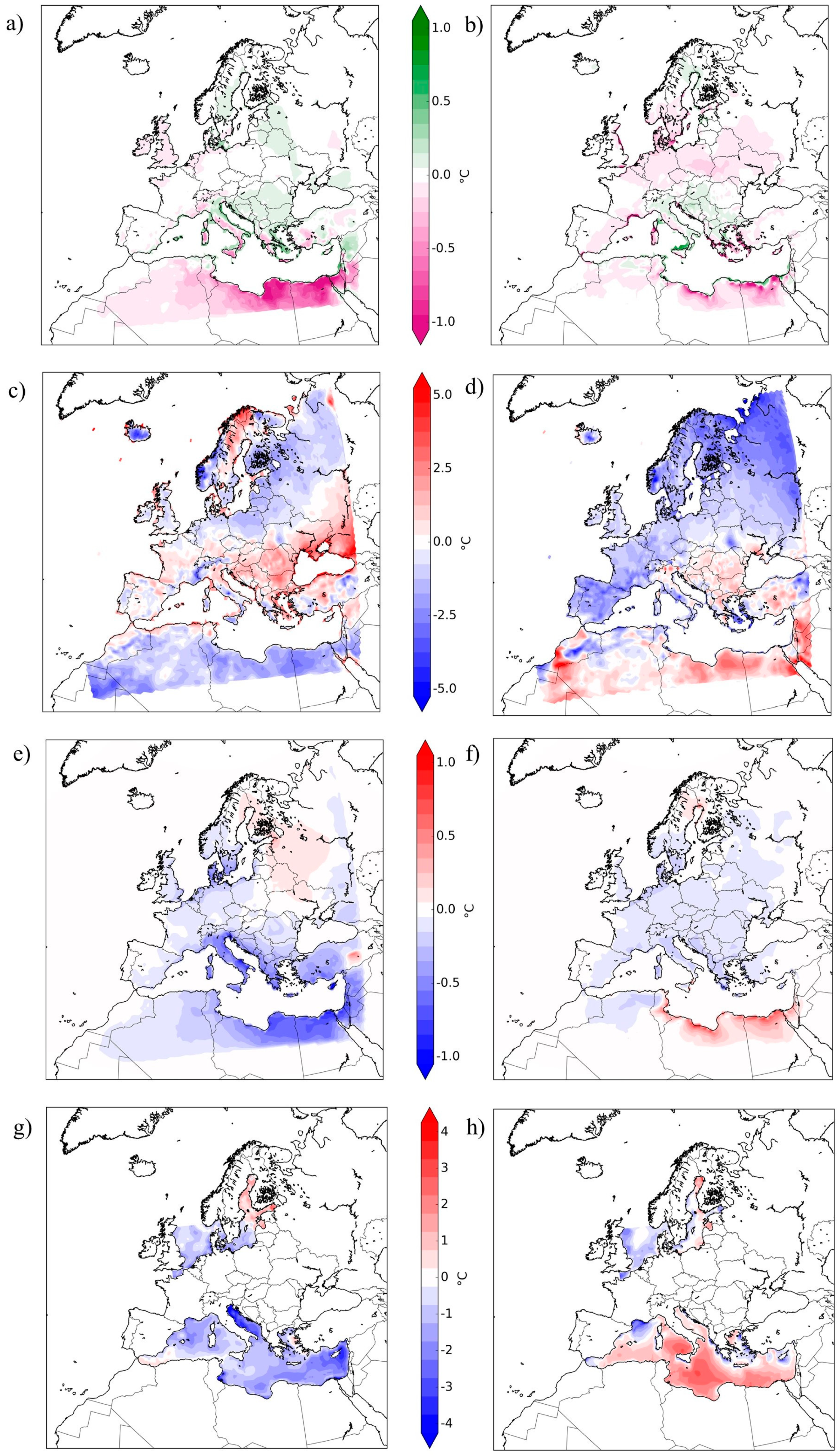
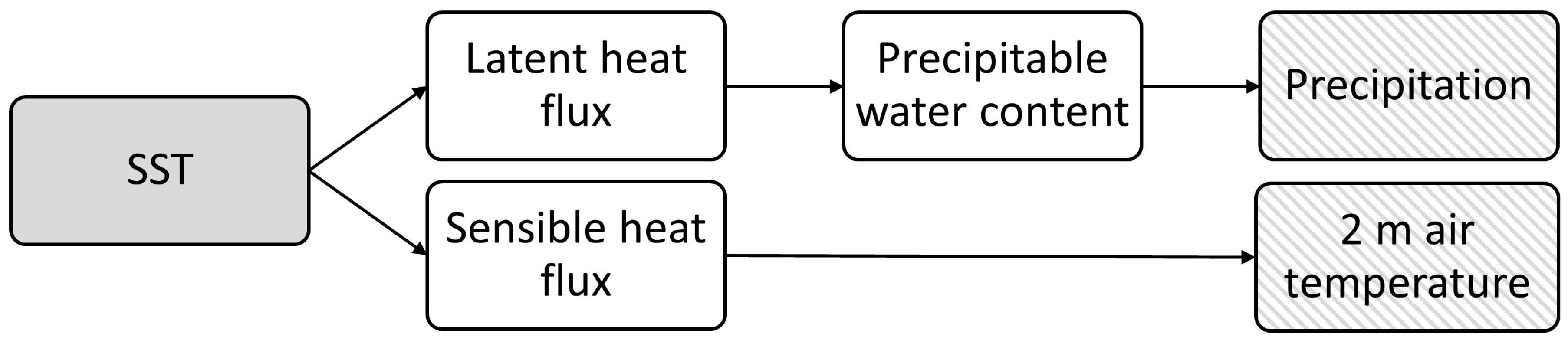
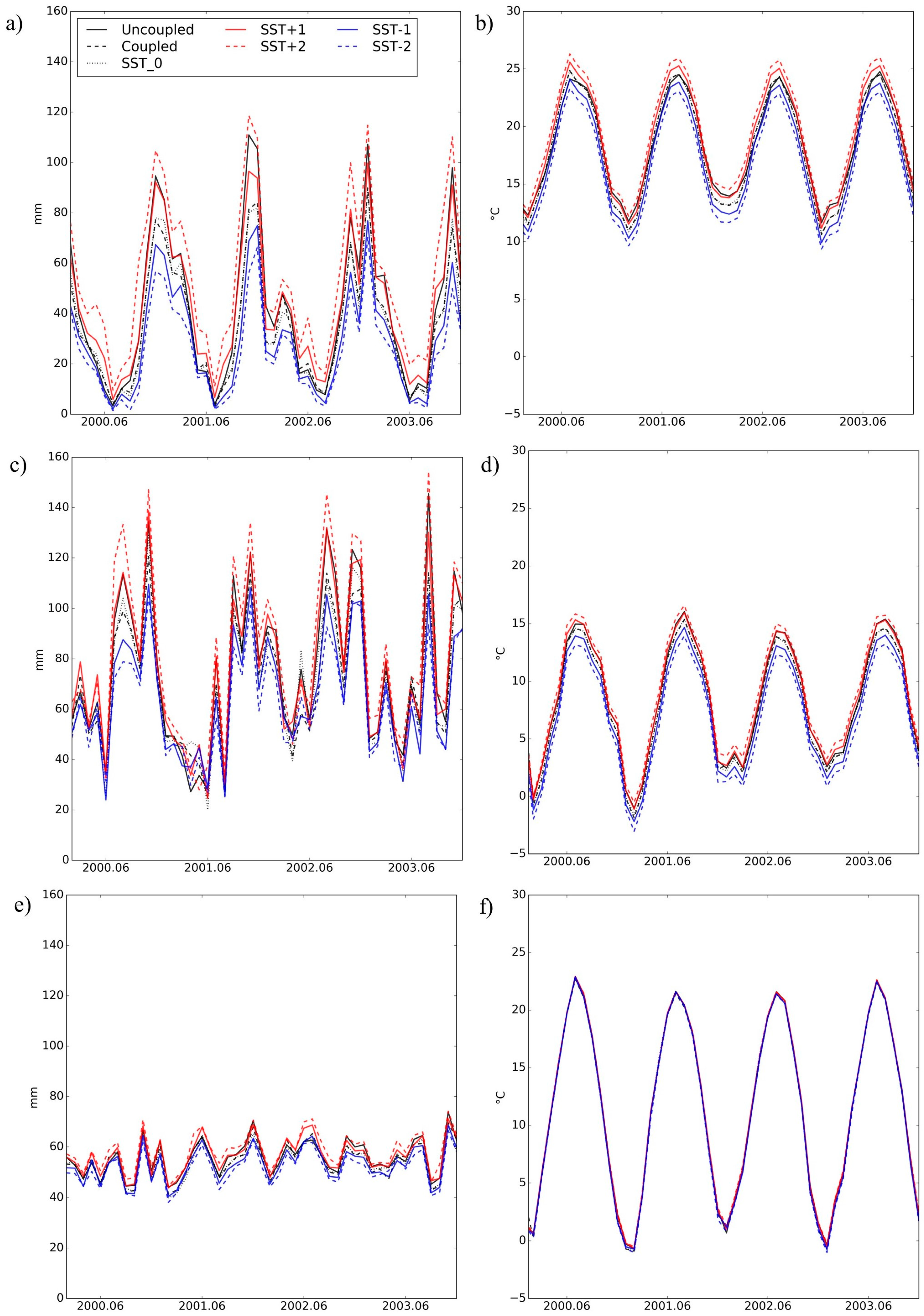
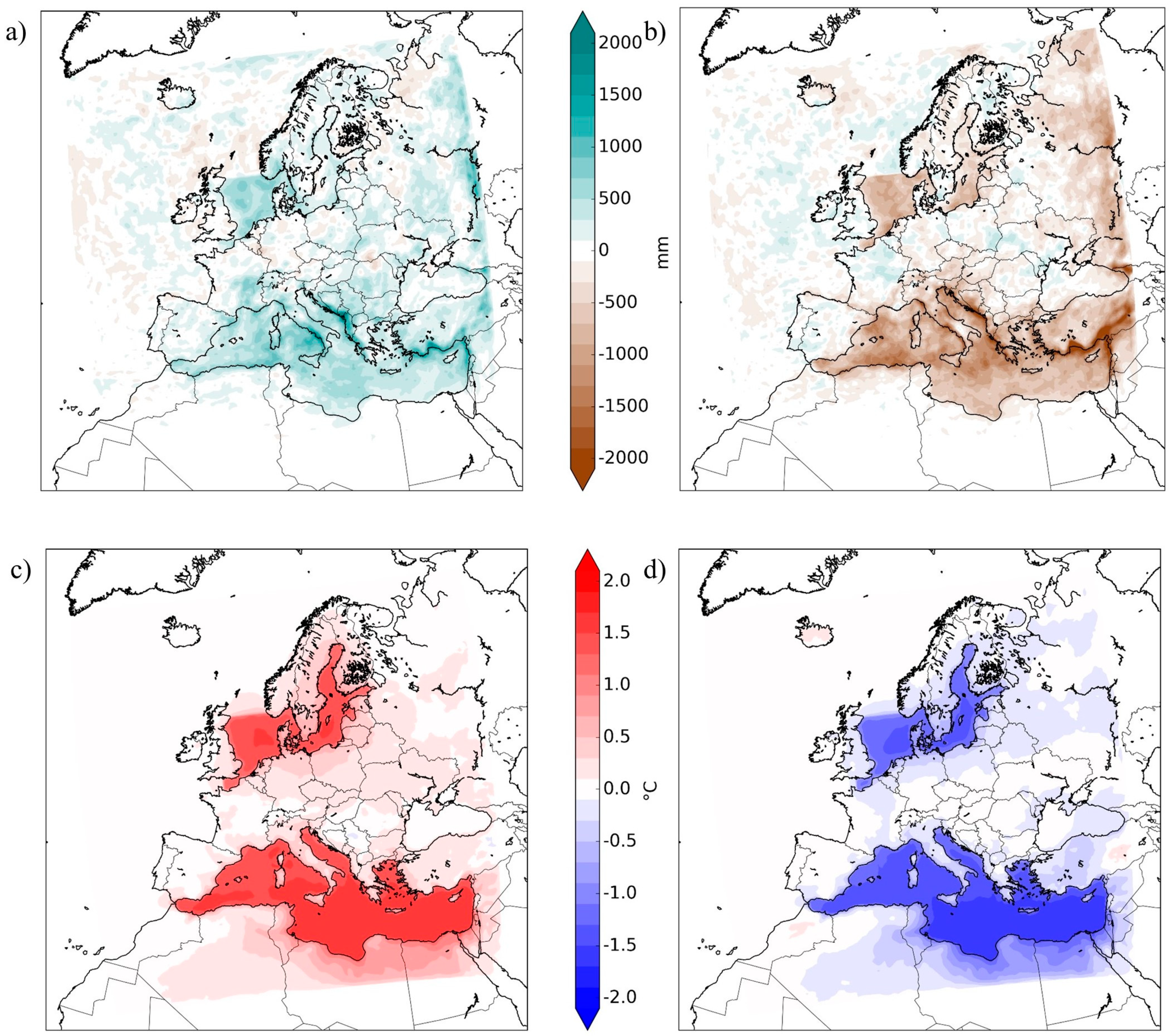
- How sensitive is the atmosphere, namely the precipitation and 2 m temperature, to SST changes in the model system?Based on our sensitivity experiments with altered SST values, we conclude that both precipitation and 2 m temperature react to SST changes. The changes are mostly over the sea areas, but some differences appear over land as well. Additionally, over continental areas precipitation seems to be more affected than 2 m temperature.
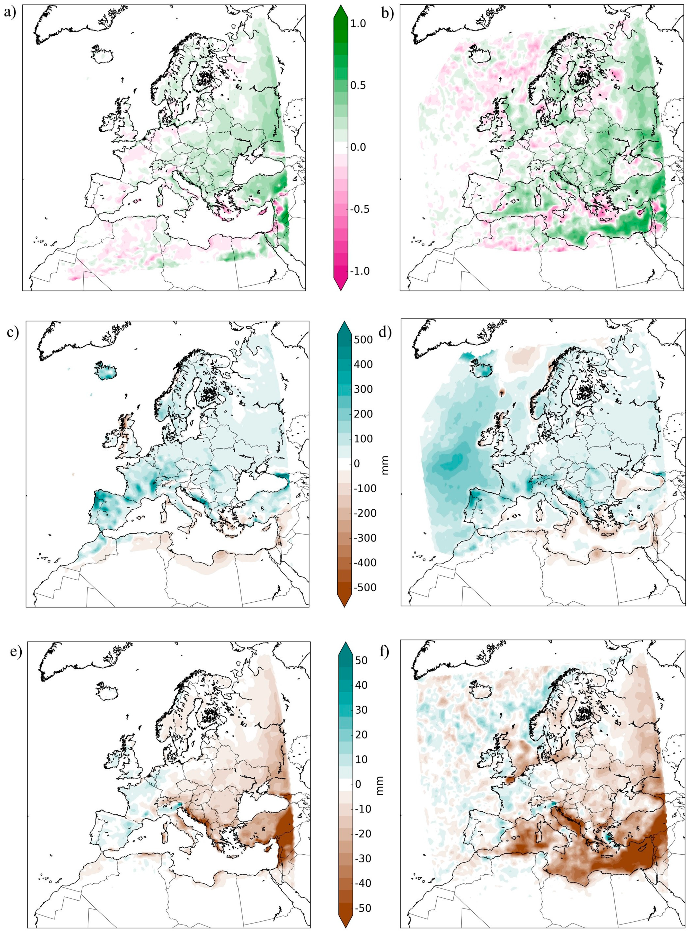
- Has the interactive coupling of atmosphere and ocean an effect over the continental areas?Yes, it has. As expected from the sensitivity experiments, precipitation is influenced by the coupling. Nevertheless, it is unclear if the difference over continental regions is due to the model’s specific feature or the result of the length of the simulation, since the century-long simulation enables the slow parts of the system to evolve and show their effect on the results. This is also an important finding to prove the importance of marginal seas further away from the coasts.
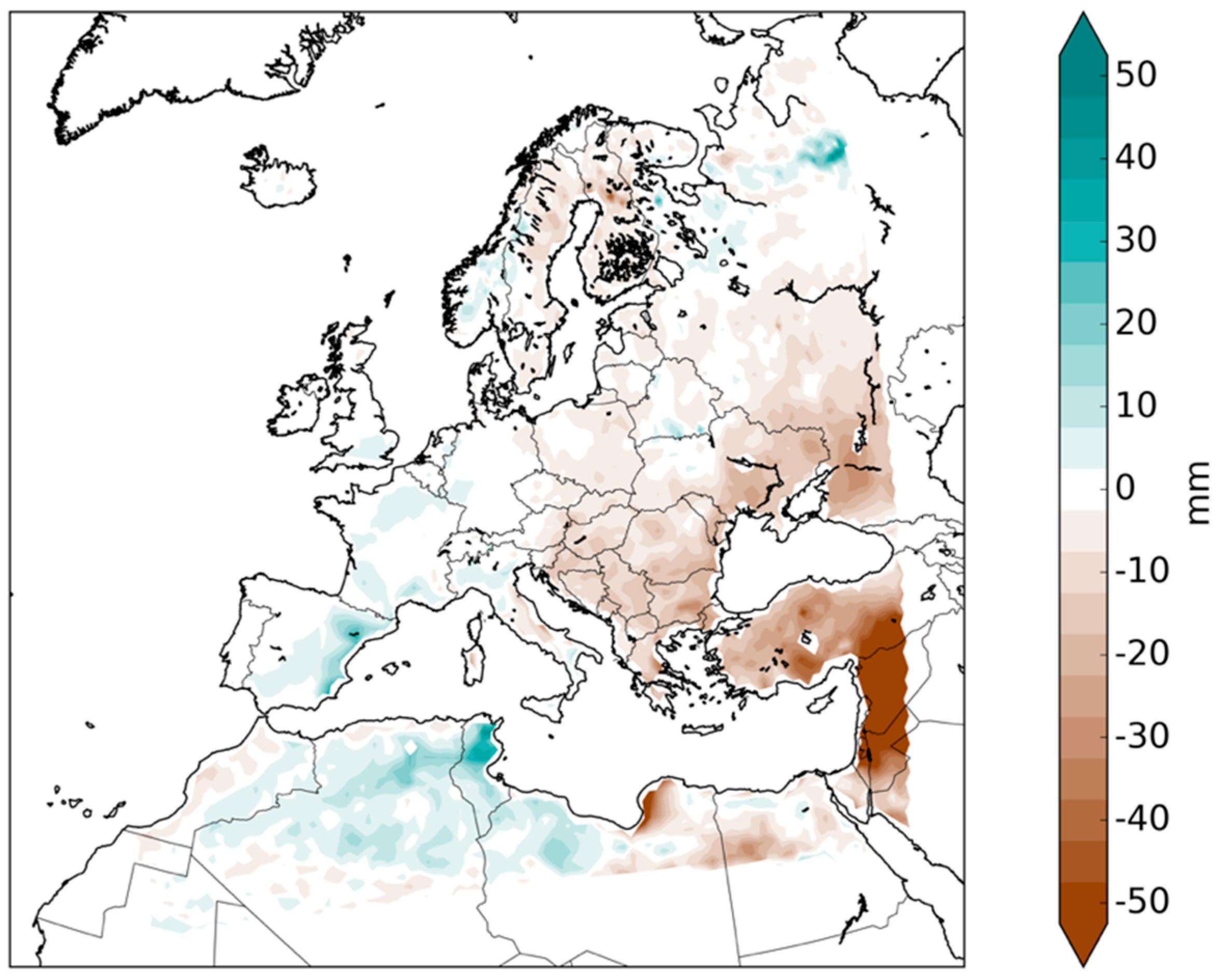
- Is there any large scale added skill in the precipitation and in the 2 m temperature variables in the coupled simulation compared to the uncoupled one?Yes, during winter the precipitation has positive skill over the eastern part of the domain. We found that the coupled system has in average a bit colder SST values than the atmosphere-only version. This leads to less precipitation, meaning smaller wet bias during winter over the eastern part of the domain. This, together with a soil moisture-evapotranspiration-precipitation positive feedback loop results in a homogenous increase in skill over a large area. In terms of 2 m temperature, we found only moderate skill in Europe.
Author Contributions
Funding
Acknowledgments
Conflicts of Interest
References
- Giorgi, F.; Mearns, L.O. Approaches to the simulation of regional climate change: A review. Rev. Geophys. 1991, 29, 191–216. [Google Scholar] [CrossRef]
- Feser, F.; Rrockel, B.; Storch, H.; Winterfeldt, J.; Zahn, M. Regional climate models add value to global model data a review and selected examples. Bull. Am. Meteorol. Soc. 2011, 92, 1181–1192. [Google Scholar] [CrossRef]
- Li, L.; Bozec, A.; Somot, S.; Beranger, K.; Bouruet-Aubertot, P.; Sevault, F.; Crepon, M. Regional atmospheric, marine processes and climate modelling. In Mediterranean Climate Variability; Lionello, P., Malanotte, R., Eds.; Elsevier B.V: Amsterdam, The Netherlands, 2006; pp. 373–397. [Google Scholar]
- Somot, S.; Sevault, F.; Déqué, M.; Crépon, M. 21st century climate change scenario for the Mediterranean using a coupled atmosphere-ocean regional climate model. Glob. Planet. Change 2008, 63, 112–126. [Google Scholar] [CrossRef]
- Van Pham, T.; Brauch, J.; Dieterich, C.; Frueh, B.; Ahrens, B. New coupled atmosphere-ocean-ice system COSMO-CLM/NEMO: Assessing air temperature sensitivity over the North and Baltic Seas. Oceanologia 2014, 56, 167–189. [Google Scholar] [CrossRef]
- Rinke, A.; Gerdes, R.; Dethloff, K.; Kandlbinder, T.; Karcher, M.; Kauker, F.; Frickenhaus, S.; Köberle, C.; Hiller, W. A case study of the anomalous Arctic sea ice conditions during 1990: Insights from coupled and uncoupled regional climate model simulations. J. Geophys. Res. Atmos. 2003, 108, 4275. [Google Scholar] [CrossRef]
- Akhtar, N.; Brauch, J.; Dobler, A.; Béranger, K.; Ahrens, B. Medicanes in an ocean-atmosphere coupled regional climate model. Nat. Hazards Earth Syst. Sci. 2014, 14, 2189–2201. [Google Scholar] [CrossRef]
- Giorgi, F. Climate change hot-spots. Geophys. Res. Lett. 2006, 33, 1–4. [Google Scholar] [CrossRef]
- Artale, V.; Calmanti, S.; Carillo, A.; Dell’Aquila, A.; Herrmann, M.; Pisacane, G.; Ruti, P.M.; Sannino, G.; Struglia, M.V.; Giorgi, F.; et al. An atmosphere-ocean regional climate model for the Mediterranean area: Assessment of a present climate simulation. Clim. Dyn. 2010, 35, 721–740. [Google Scholar] [CrossRef]
- Drobinski, P.; Anav, A.; Brossier, C.L.; Samson, G.; Stéfanon, M.; Bastin, S.; Baklouti, M.; Béranger, K.; Beuvier, J.; Bourdallé-Badie, R.; et al. Model of the Regional Coupled Earth system (MORCE): Application to process and climate studies in vulnerable regions. Environ. Model. Softw. 2012, 35, 1–18. [Google Scholar] [CrossRef]
- Lebeaupin Brossier, C.; Drobinski, P.; Béranger, K.; Bastin, S.; Orain, F. Ocean memory effect on the dynamics of coastal heavy precipitation preceded by a mistral event in the northwestern Mediterranean. Q. J. R. Meteorol. Soc. 2013, 139, 1583–1597. [Google Scholar] [CrossRef]
- Lebeaupin Brossier, C.; Béranger, K.; Deltel, C.; Drobinski, P. The Mediterranean response to different space-time resolution atmospheric forcings using perpetual mode sensitivity simulations. Ocean Model. 2011, 36, 1–25. [Google Scholar] [CrossRef]
- Sevault, F.; Somot, S.; Alias, A.; Dubois, C.; Lebeaupin-Brossier, C.; Nabat, P.; Adloff, F.; Déqué, M.; Decharme, B. A fully coupled Mediterranean regional climate system model: design and evaluation of the ocean component for the 1980–2012 period. Tellus A Dyn. Meteorol. Oceanogr. 2014, 66, 23967. [Google Scholar] [CrossRef]
- Döös, K.; Meier, H.E.M.; Döscher, R. The Baltic Haline Conveyor Belt or The Overturning Circulation and Mixing in the Baltic. AMBIO A J. Hum. Environ. 2009, 33, 261–266. [Google Scholar] [CrossRef]
- Daewel, U.; Schrum, C. Simulating long-term dynamics of the coupled North Sea and Baltic Sea ecosystem with ECOSMO II: Model description and validation. J. Mar. Syst. 2013, 119–120, 30–49. [Google Scholar] [CrossRef]
- Schrum, C.; Hübner, U.; Jacob, D.; Podzun, R. A coupled atmosphere/ice/ocean model for the North Sea and the Baltic Sea. Clim. Dyn. 2003, 21, 131–151. [Google Scholar] [CrossRef]
- Doscher, R.; Willén, U.; Jones, C.; Rutgersson, A.; Meier, H.M.; Hansson, U.; Graham, L.P. The development of the regional coupled ocean-atmosphere model RCAO. Boreal Environ. Res. 2002, 7, 183–192. [Google Scholar]
- Dieterich, C.; Wang, S.; Schimanke, S.; Gröger, M.; Klein, B.; Hordoir, R.; Samuelsson, P.; Liu, Y.; Axell, L.; Höglund, A.; et al. Surface Heat Budget over the North Sea in Climate Change Simulations. Atmosphere (Basel). 2019, 10, 272. [Google Scholar] [CrossRef]
- Primo, C.; Kelemen, F.D.; Feldmann, H.; Ahrens, B. A regional atmosphere-ocean climate system model over Europe including three marginal seas: On its stability and performance. Geosci. Model Dev. 2019, 1–33. [Google Scholar] [CrossRef]
- Akhtar, N.; Brauch, J.; Ahrens, B. Climate modeling over the Mediterranean Sea: impact of resolution and ocean coupling. Clim. Dyn. 2018, 51, 933–948. [Google Scholar] [CrossRef]
- Gröger, M.; Dieterich, C.; Meier, M.H.E.; Schimanke, S. Thermal air-sea coupling in hindcast simulations for the North Sea and Baltic Sea on the NW European shelf. Tellus Ser. A Dyn. Meteorol. Oceanogr. 2015, 67, 1. [Google Scholar] [CrossRef]
- Rockel, B.; Castro, C.L.; Pielke, R.A.; von Storch, H.; Leoncini, G. Dynamical downscaling: Assessment of model system dependent retained and added variability for two different regional climate models. J. Geophys. Res. 2008, 113, 1–9. [Google Scholar] [CrossRef]
- Doms, G.; Förstner, J.; Heise, E.; Herzog, H.J.; Mironov, D.; Raschendorfer, M.; Reinhardt, T.; Ritter, B.; Schrodin, R.; Schulz, J.P.; et al. A Description of the Nonhydrostatic Regional COSMO Model Part II: Physical Parameterization. In Consortium for Small-Scale Modelling; Deutscher Wetterdienst: Offenbach, Germany, 2011; p. 154. [Google Scholar]
- Giorgi, F.; Jones, C.; Asrar, G.R. Addressing climate information needs at the regional level: the CORDEX framework. World Meteorol. Organ. Bull. 2009, 58, 175–183. [Google Scholar]
- Müller, W.A.; Pohlmann, H.; Sienz, F.; Smith, D. Decadal climatepredictions for theperiod1901–2010 with a coupled climate model. Geophys. Res. Lett. 2014, 41, 2100–2107. [Google Scholar] [CrossRef]
- Müller, W.A.; Matei, D.; Bersch, M.; Jungclaus, J.H.; Haak, H.; Lohmann, K.; Compo, G.P.; Sardeshmukh, P.D.; Marotzke, J. A twentieth-century reanalysis forced ocean model to reconstruct the North Atlantic climate variation during the 1920s. Clim. Dyn. 2015, 44, 1935–1955. [Google Scholar] [CrossRef]
- Compo, G.P.; Whitaker, J.S.; Sardeshmukh, P.D.; Matsui, N.; Allan, R.J.; Yin, X.; Gleason, B.E.; Vose, R.S.; Rutledge, G.; Bessemoulin, P.; et al. The Twentieth Century Reanalysis Project. Q. J. R. Meteorol. Soc. 2011, 137, 1–28. [Google Scholar] [CrossRef]
- Rayner, N.A. Global analyses of sea surface temperature, sea ice, and night marine air temperature since the late nineteenth century. J. Geophys. Res. 2003, 108, 4407. [Google Scholar] [CrossRef]
- Beuvier, J.; Brossier, C.L.; Béranger, K.; Arsouze, T.; Bourdallé-Badie, R.; Deltel, C.; Drillet, Y.; Drobinski, P.; Ferry, N.; Lyard, F.; et al. MED12, oceanic component for the modeling of the regional Mediterranean earth system. Mercat. Ocean Q. Newsl. 2012, 46, 60–66. [Google Scholar]
- Hordoir, R.; Axell, L.; Höglund, A.; Dieterich, C.; Fransner, F.; Groger, M.; Liu, Y.; Pemberton, P.; Schimanke, S.; Andersson, H.; et al. Nemo-Nordic 1.0: A NEMO-based ocean model for the Baltic and North seas - Research and operational applications. Geosci. Model Dev. 2019, 12, 363–386. [Google Scholar] [CrossRef]
- Vancoppenolle, M.; Fichefet, T.; Goosse, H.; Bouillon, S.; Madec, G.; Maqueda, M.A.M. Simulating the mass balance and salinity of Arctic and Antarctic sea ice. 1. Model description and validation. Ocean Model. 2009, 27, 33–53. [Google Scholar] [CrossRef]
- Craig, A.; Valcke, S.; Coquart, L. Development and performance of a new version of the OASIS coupler, OASIS3-MCT-3.0. Geosci. Model Dev. 2017, 10, 3297–3308. [Google Scholar] [CrossRef]
- Harris, I.; Jones, P.D.; Osborn, T.J.; Lister, D.H. Updated high-resolution grids of monthly climatic observations - the CRU TS3.10 Dataset. Int. J. Climatol. 2014, 34, 623–642. [Google Scholar] [CrossRef]
- Andersson, A.; Ziese, M.; Dietzsch, F.; Schröder, M.; Becker, A.; Schamm, K. HOAPS/GPCC European daily precipitation data record with uncertainty estimates using satellite and gauge based observations at 0.5°. Glob. Precip. Climatol. Cent. Dtsch. Wetterd. 2016. [Google Scholar] [CrossRef]
- Murphy, A.H. Skill scores based on the mean square error and their relationships to the correlation coefficient. Mon. Weather Rev. 1988, 116, 2417–2424. [Google Scholar] [CrossRef]
- Schär, C.; Lüthi, D.; Beyerle, U.; Heise, E. The soil-precipitation feedback: A process study with a regional climate model. J. Clim. 1999, 12, 722–741. [Google Scholar] [CrossRef]
- Panthou, G.; Vrac, M.; Drobinski, P.; Bastin, S.; Li, L. Impact of model resolution and Mediterranean sea coupling on hydrometeorological extremes in RCMs in the frame of HyMeX and MED-CORDEX. Clim. Dyn. 2018, 51, 915–932. [Google Scholar] [CrossRef]


| Experiment Name | Uncoupled | Coupled | SST_0 | SST + 1 | SST – 1 | SST + 2 | SST – 2 |
|---|---|---|---|---|---|---|---|
| Model | CCLM | CCLM-NEMO | CCLM | CCLM | CCLM | CCLM | CCLM |
| SST (marginal seas) | MPI-ESM-LR as20ncep08 | SST from NEMO (CPL SST) | CPL SST | CPL SST + 1 | CPL SST – 1 | CPL SST + 2 | CPL SST – 2 |
© 2019 by the authors. Licensee MDPI, Basel, Switzerland. This article is an open access article distributed under the terms and conditions of the Creative Commons Attribution (CC BY) license (http://creativecommons.org/licenses/by/4.0/).
Share and Cite
Kelemen, F.D.; Primo, C.; Feldmann, H.; Ahrens, B. Added Value of Atmosphere-Ocean Coupling in a Century-Long Regional Climate Simulation. Atmosphere 2019, 10, 537. https://doi.org/10.3390/atmos10090537
Kelemen FD, Primo C, Feldmann H, Ahrens B. Added Value of Atmosphere-Ocean Coupling in a Century-Long Regional Climate Simulation. Atmosphere. 2019; 10(9):537. https://doi.org/10.3390/atmos10090537
Chicago/Turabian StyleKelemen, Fanni Dóra, Cristina Primo, Hendrik Feldmann, and Bodo Ahrens. 2019. "Added Value of Atmosphere-Ocean Coupling in a Century-Long Regional Climate Simulation" Atmosphere 10, no. 9: 537. https://doi.org/10.3390/atmos10090537
APA StyleKelemen, F. D., Primo, C., Feldmann, H., & Ahrens, B. (2019). Added Value of Atmosphere-Ocean Coupling in a Century-Long Regional Climate Simulation. Atmosphere, 10(9), 537. https://doi.org/10.3390/atmos10090537