Article

Added Value of Atmosphere-Ocean Coupling in a Century-Long Regional Climate Simulation

1
Institute for Atmospheric and Environmental Sciences, Goethe University, 60438 Frankfurt am Main, Germany
2
Institute of Meteorology and Climate Research, Karlsruhe Institute of Technology, 76021 Karlsruhe, Germany
*
Author to whom correspondence should be addressed.
Atmosphere 2019, 10(9), 537; https://doi.org/10.3390/atmos10090537
Submission received: 1 July 2019 / Revised: 6 September 2019 / Accepted: 8 September 2019 / Published: 11 September 2019
(This article belongs to the Special Issue Regional Climate Modeling: Ocean–Atmosphere Coupling)

Abstract

:
A twentieth century-long coupled atmosphere-ocean regional climate simulation with COSMO-CLM (Consortium for Small-Scale Modeling, Climate Limited-area Model) and NEMO (Nucleus for European Modelling of the Ocean) is studied here to evaluate the added value of coupled marginal seas over continental regions. The interactive coupling of the marginal seas, namely the Mediterranean, the North and the Baltic Seas, to the atmosphere in the European region gives a comprehensive modelling system. It is expected to be able to describe the climatological features of this geographically complex area even more precisely than an atmosphere-only climate model. The investigated variables are precipitation and 2 m temperature. Sensitivity studies are used to assess the impact of SST (sea surface temperature) changes over land areas. The different SST values affect the continental precipitation more than the 2 m temperature. The simulated variables are compared to the CRU (Climatic Research Unit) observational data, and also to the HOAPS/GPCC (Hamburg Ocean Atmosphere Parameters and Fluxes from Satellite Data, Global Precipitation Climatology Centre) data. In the coupled simulation, added skill is found primarily during winter over the eastern part of Europe. Our analysis shows that, over this region, the coupled system is dryer than the uncoupled system, both in terms of precipitation and soil moisture, which means a decrease in the bias of the system. Thus, the coupling improves the simulation of precipitation over the eastern part of Europe, due to cooler SST values and in consequence, drier soil.

1. Introduction

High-resolution climatological data is essential for studying the climate system’s features and its changes—both in the past and in the future. Thus, a significant effort is taken into improving climate models, which can provide us with the sufficient data. One way of improvement in climate research is the development and usage of regional climate models (RCM), or limited area models [1]. These models enable us to increase the spatial resolution of simulations without being as expensive as global models on the same high resolution. Moreover, RCMs are able to resolve more regional scale climate processes, due to their high resolution [2]. One further step in the improvement is the use of regional climate system models (RCSM). This means that not only the atmosphere and land surface, but also other parts of the climate system are modelled in detail by numerical models and coupled together in an interactive way. Depending on the focus of a study, the coupled system could include several elements of the climate system. Since the changes undergoing in the ocean have great relevance on the climate timescale, the coupling of an atmosphere and an ocean model is one often-used combination.
The advantage of a regional atmosphere-ocean coupled climate model is that it is physically more consistent with the natural system than an atmosphere-only climate model. The ocean model has the resolution to better represent the regional features of the marginal seas (such as the Mediterranean or the Baltic Sea) than an uncoupled RCM, which uses SST (sea surface temperature) data either from the driving model or from a reanalysis to represent the ocean [3,4]. The interactive coupling also enables a more realistic dynamical response to perturbations regarding the ocean atmosphere heat balance. Thus, we expect that a coupled model system can better adapt to changes or feedback mechanisms, which is favorable in both hindcast simulations and in future projections. With a coupled marginal sea, an RCSM is also more independent from its driving global model and its biases. Nevertheless, the coupling extends the complexity, and also the cost of calculations, so the more diverse system might not always improve all variables.
Chronologically, coupling atmosphere and ocean global circulation models (AOGCMs) have started among the global climate models, due to the increasing need in climate science to take into consideration more aspects of the climate system, especially those having longer memory (decades or centuries). The Coupled Model Intercomparison Project (CMIP) began in 1995 under the auspices of the Working Group on Coupled Modelling (WGCM). Since then, the sixth phase of the project has already been engaged, and coupled AOGCMs are considered the state-of-the-art climate models. The application of coupling among the regional climate models is also increasing, focusing over regions where marginal seas influence the local climate, e.g., the Baltic Sea, the Arctic or the Mediterranean [5,6,7].
In Europe, the biggest marginal sea is the Mediterranean Sea, which has a great influence on its environment. It is an important moisture and heat source. The Mediterranean climate is characterized by a dry summer and a wet winter as it is affected by the downdraft part of the Hadley cell during summer and the mid-latitude Westerlies during winter. The dry summer, projected to be even dryer in the future, lets the Mediterranean region to be considered as a climate change ‘hot spot’ [8]. Thus, the successful modelling of its climate is crucial for climate change projections. Furthermore, the regional characteristics of the Mediterranean basin also leads to the formation of high impact weather phenomena, such as topographically-induced strong winds, intense cyclogenesis or heavy precipitation, which are all also influenced by the interaction between air and sea. To better resolve the interaction between the atmosphere and the Mediterranean Sea, Reference [4] coupled a global atmosphere model (ARPEGE) locally to a regional ocean model (OPAMED) over the Mediterranean. There are also studies coupling regional atmosphere and regional ocean models, such as the work from Reference [9], where the atmosphere component is the RegCM3, and the Mediterranean Sea is represented by MITgcm. Reference [10] created a regional coupled earth system model with the components: WRF (atmosphere) and NEMO (Nucleus for European Modelling of the Ocean)(ocean), which was also used to examine the air-sea interactions and the role of the general ocean circulation in two intense weather events in the Mediterranean [11]. The NEMO ocean model has a regional configuration over the Mediterranean Sea, NEMO-MED12 [12], which was coupled to the atmosphere model COSMO-CLM (Consortium for Small-Scale Modeling, Climate Limited-area Model) to study medicanes, where the coupled system showed improvements compared to the atmosphere-only simulations [7]. Reference [13] coupled NEMO with a different atmosphere model (CNRM-ALADIN52) and even included a river routing model (TRIP) into the regional climate system.
Another semi-enclosed marginal sea in Europe is the Baltic Sea, which connects to the North Sea. The Baltic Sea has different characteristics from the Mediterranean, but they both have a notable influence on the weather and the climate of their surroundings. The Baltic Sea has a strongly stratified characteristic, which is influenced by freshwater and nutrient input from continental rivers and has a residence time of the order of 25–30 years [14]. In addition, the sea ice formation is significant over the Baltic Sea, a process that does not have to be considered in the Mediterranean Sea. The Baltic Sea is directly connected to the North Sea, which in contrast to the Baltic Sea, is a dynamical region. Neither the oceanographical, nor the biogeochemical characteristics of the Baltic and the North Seas are similar, but they are closely linked to each other. Reference [15] showed that modelling them together gives a better representation of the seas than trying to assess the in- and outflow separately. Similarly to the Mediterranean region, in this area, it is potentially favorable to use a coupled atmosphere ocean regional model. Reference [16] coupled regional atmosphere/ice/ocean models (REMO and HAMSOM) in the Baltic and North Sea region. They found that the system is stable over a full seasonal cycle. Moreover, its results showed improvements compared to the results of the uncoupled, atmospheric model. Reference [17] coupled different regional models (RCO and RCA) only for the Baltic Sea, but focus on a multi-year simulation to analyze the possibility of climate studies. Reference [5] downscaled 20 years of ERA-Interim reanalysis with a coupled atmosphere-ocean-ice system (COSMO-CLM for atmosphere and NEMO for the ocean with the sea ice module LIM3), where both the Baltic and the North Seas were included in the coupling. Recently, Reference [18] investigated future scenarios of the North Sea with the coupled atmosphere–ice–ocean model RCA4-NEMO.
In this study, we evaluate the added value of a coupled atmosphere-ocean-ice simulation, where three marginal seas, namely the Mediterranean, the Baltic and the North Seas are calculated dynamically. Moreover, the simulation has been calculated for more than 100 years including the whole twentieth century. With the coupling of three marginal seas, which means the majority of the ocean grid points in our domain, one expects the model to become better in describing the dynamical system. The motivation for a twentieth century simulation is that it gives the opportunity to study longer trends and extremes with large return periods. Modelled data is needed for this, since observational data is not always available for this time range, or it has only low resolution, as well as available only over land. The stability of the simulation during the twentieth century is evaluated in Reference [19], where the authors present that the climate system is stable, and it does not have any continuous drift. Nevertheless, it is not free from biases. In coupled simulations, the differences and added value are mainly located close to the coupled sea, along the coast or over islands [20,21]. Despite this, a transient century-long simulation might show some improvements also over the continental region, since the system has a long time to adapt and progress with the more complex climate system dynamics. Reference [19] analyze the effect of coupling regarding extremes with the help of daily observations from Germany stations. They found, that in Germany the coupled system improves the values of the climate change indices related to extreme temperatures compared to the uncoupled version, while for related precipitation indices the uncoupled simulation is more skillful. In this study, we extend their analysis by focusing on the added value over all land areas in Europe, while, due to the lack of adequate observations, we do not analyze extremes. Our focus is on the atmospheric side of the climate variables, namely on precipitation and 2 m temperature on a seasonal timescale.
The research questions, we want to answer in this study are:
  • How sensitive is the atmosphere, namely the precipitation and 2 m temperature, to SST changes in the model system?
  • Does the interactive coupling of atmosphere and ocean have an effect over the continental areas?
  • Is there any large-scale added skill in the precipitation and in the 2 m temperature variables in the coupled simulation compared to the uncoupled one?
The next section describes the uncoupled and coupled simulations, together with the observations used as reference data. Section 3 introduces the sensitivity studies, designed to answer our first research question, and explains the skill score used to quantify the added value. Section 4 presents the results from our sensitivity studies and from the analysis of the century-long simulations. The last section discusses and summarizes the work and concludes the results presented in this paper.

2. Data

In this study, we compare the results of a coupled atmosphere-ocean regional climate model to its uncoupled counterpart. The atmosphere-only simulation dynamically resolves the processes in the atmosphere and uses boundary conditions from a global earth system model to gain information regarding the status of the ocean and seas. On the other hand, the coupled atmosphere-ocean simulation resolves the dynamical processes also in the Mediterranean, the Baltic and the North Seas. Both the coupled and the uncoupled simulations are calculated for the twentieth century. To evaluate the results, observations are used as reference data.

2.1. Uncoupled Simulation

The atmosphere model used in the uncoupled/standalone simulation is the climate version of the non-hydrostatic limited-area atmospheric prediction model COSMO-CLM (CCLM, Consortium for Small-Scale Modeling, Climate Limited-area Model) [22] developed by the German Weather Service (Deutscher Wetterdienst, DWD). For the simulation, CCLM v5.0 clm7 was used. The model uses the primitive thermo-hydrodynamical equations describing compressible flow in a moist atmosphere. In our simulations with CCLM, the interaction between the atmosphere and the underlying surface is modelled by a soil and vegetation Model, TERRA [23].
The domain, EURO-CORDEX, is defined within the CORDEX framework (Coordinated Regional climate Downscaling Experiment) [24], and, in our case, the spatial resolution is 0.22° × 0.22° (~25 km) with 40 vertical levels. The twentieth century simulation covers the period between 1 January 1900 and 31 December 2009.
For the regional simulation, global driving data is needed. The driving data is taken 6-hourly from the Max Planck Institute Earth System Model used in the low-resolution configuration (MPI-ESM-LR). The simulation used in our study is called an assimilation experiment (as20ncep08) [25], because the model state is nudged towards three dimensional daily ocean temperature and salinity anomalies coming from an ocean only model simulation [26]. The ocean only simulation is calculated with the Max Planck Institute Ocean Model (MPIOM) forced with a twentieth century reanalysis of the atmosphere (20CR) [27]. In MPI-ESM-LR the horizontal resolution of the atmosphere is approximately 200 km at 47 layers, and the ocean varies from 12 to 150 km at 40 layers. In the Mediterranean region, the ocean model’s resolution is around 100 km, and it becomes denser around the poles, thus, at the North and Baltic Sea region it has higher resolution than at the Mediterranean Sea. For our study, it is important to keep in mind what kind of SST data is used in the uncoupled experiment, since that is one of the main differences between the coupled and uncoupled simulations. So, we follow the information flow to show the origin of the uncoupled regional simulation’s SST boundary conditions. The SST boundary conditions consist of the MPI-ESM-LR model climatology plus the anomalies coming from the MPIOM 20CR assimilation experiment. The ocean model is forced by a number of different parameters to obtain fluxes of heat, momentum and freshwater [26]. Particularly, for the calculation of latent and heat fluxes, the MPIOM uses surface and 2 m temperature from 20CR. The SST values in the 20CR reanalysis are taken from the UK Met Office HadISST1.1 (Hadley Centre sea ice and sea surface temperature) dataset [28], as the atmosphere-land model system, creating the reanalysis needed lower boundary conditions. Thus, the SST values used in our uncoupled experiment are in the end originated from the HadISST dataset, but as our previous study [19] shows, the SST values in the global and uncoupled system have a cold bias compared to the observations. Nevertheless, they are not independent from the observed data.

2.2. Coupled Simulation

The coupled simulation evaluated in our study consist of three main models, CCLM responsible for the atmosphere and land surface, NEMO-MED12 [29] for the Mediterranean Sea and NEMO-NORDIC [30] for the Baltic and North Seas. Moreover, NEMO-NORDIC also includes a sea ice model named LIM3 (Louvain-la-Neuve sea ice model) [31]. The different models are coupled with the OASIS3-MCT (Ocean Atmosphere Sea Ice Soil Model Coupling Toolkit; [32]), which coordinates the technical part of the coupling. One of the challenges of the coupling, which is handled by OASIS3-MCT, is that the three models have different spatial resolutions: CCLM has the same resolution (~25km) as the uncoupled simulation, NEMO-MED12 has a spatial resolution of 1/12° (~9km), and NEMO-NORDIC is integrated on the highest resolution (~3 km). The coupling means that variables are interchanged between the models every 3 h. In our case, the atmosphere model receives the SST and in the case of the Baltic and North Seas region also the sea ice fraction from the ocean models. On the other hand, the atmosphere model transmits to the ocean models the flux densities of water (precipitation-evaporation), momentum, solar radiation, non-solar energy and in the case of the Baltic and North Seas region also the sea level pressure. The coupled system gets its driving data at the boundaries from the same assimilation experiment of MPI-ESM-LR as the uncoupled simulation. To illustrate the computational side of running a coupled system, Reference [19] calculated for how long does the coupled and the uncoupled system run when using the same resources (same amount of nodes for the whole system), and they found that the coupled system needs ca. five times more time for the integration. For more details on the coupled system, we also refer to Reference [19], who investigated the stability of the same simulations.

2.3. Observations

As our objective is to evaluate the added value in the century-long simulation, we need a comparably long observational dataset all over Europe for reference. This requirement is filled by the high resolution gridded dataset of the Climatic Research Unit (CRU TS) [33]. The CRU TS4.01 dataset is available between 1901 and 2016, but we used the data only until 2009, when our simulations end. The CRU high resolution dataset is a gridded dataset constructed from monthly meteorological station observations. It covers the land areas worldwide with a 0.5° latitude/longitude grid. The dataset contains six climate variables; from which we used only precipitation and daily mean temperature.
The disadvantage of the CRU dataset is that it is land-only, since it contains century-long station data, which are not available over marine areas. Nevertheless, for a coupled simulation’s evaluation, the over the sea areas are particularly interesting. To have measurements over large sea areas, one needs to rely on remote sensing, which is on the other hand not available for such a long time as ground-based measurements. Thus, to be able to check the results of the coupled system over the sea, we included in our study a dataset containing precipitation observations also over the sea, but with the constraint that this analysis is only for the last decades of the century. The dataset is called HOAPS/GPCC (Hamburg Ocean Atmosphere Parameters and Fluxes from Satellite Data, Global Precipitation Climatology Centre) global daily precipitation data based on satellite and gauge based observations [34]. It is available between 1988 and 2008 over Europe on a 0.5° grid.

3. Methods

3.1. Sensitivity Studies

Our previous analysis [19] showed that the SST values in the coupled and the uncoupled system differ. Their temporal evolution through the century is similar, but their distribution and the average SST values are different in the range of 0.5 K. To put this into perspective, we calculate the spread of an 8-member ensemble of CMIP5 global models’ SST field means. We found that the ensemble spread over the Mediterranean and the Baltic and North Seas is in the range of 1–1.5 K. In addition, during the coupling process, one of the main variables given from NEMO to CCLM is SST. So, the SST variation is an important factor in the simulations. Therefore, we planned a few sensitivity experiments with perturbed SST values in the uncoupled system, to assess the response of the atmosphere to variations in SST values. This assessment helps us to put the results of the coupled system into perspective, and it gives an estimate of the atmosphere’s answer to a robust SST change. Since the model is such a complex system, we use the sensitivity experiments as a tool to enlighten the connection between SST, precipitation and 2 m temperature. They help us to define the processes taking place in the model, due to the different SST values (Figure 1). We assume that a change in SST will cause a change in the same direction in the surface sensible and latent heat fluxes. The sensible heat flux is directly connected to the 2 m air temperature values, so we would expect the air temperature to rise when the sea is warmer and vice versa. The latent heat flux describes how much water is evaporated from the surface; thus, it is in relation to the precipitable water content of the air column, which is connected to precipitation. Thus, with warmer SST, we expect that the hydrological cycle becomes more active, resulting in more precipitation, and with cooler SST that it slows down, which would mean dryer conditions. Nevertheless, the coupled system is more complex than the sensitivity experiments designed here. Other processes and feedback mechanisms related to air-sea interactions might not be considered in the offline set-up of the sensitivity experiments. Hence, the results of the coupled system cannot be explained based on these sensitivity experiments alone.
For the sensitivity experiments, the uncoupled system (CCLM standalone simulation) is restarted in 2000. For the experiments, we choose to run the model until 2003 to give time for the perturbances to evolve and to have several seasons to evaluate. The SST values are the lower boundary conditions of the model. In our sensitivity studies, we altered these boundary conditions. Five different SST conditions are prepared for the uncoupled sensitivity runs: One with the SST values from the coupled simulation and four with the coupled SST ±1 and ±2 K (see Table 1). We change the SST only in the region of the coupled marginal seas, to be consistent with the coupled system. The discontinuity can be a concern over the northern border of the North Sea, but this issue also arises in the coupled system. The SST_0 study is very close to the coupled simulation, since it uses the SST values from it, but there are two differences between the two runs. First, the frequency of SST update is higher in the coupled simulation, namely 3 h; while in the SST_0 study, we use 6 hourly boundary conditions. The other difference is that in the SST_0 study, the sea does not react to the atmosphere, since the SST is prescribed from a different set up with a different atmospheric forcing. Thus, in the SST_0 simulation, there are no two-way interactions between sea and atmosphere.
The atmospheric answer is studied through precipitation and 2 m temperature changes.

3.2. Mean Square Error Skill Score

To quantify the added value of coupling a dynamic ocean model to the RCM, we choose a skill score, namely the mean square error skill score (MSESS) [35]:
M S E S S = 1 M S E i M S E r
MSEi and MSEr are the mean square error of the simulation of interest and reference, in our case, the coupled and the uncoupled simulation, respectively. MSEi and MSEr are calculated based on observations, in our case, the CRU TS4.01 dataset. This skill score concentrates the coupled, the uncoupled and the observation data. It shows, when positive, if the coupled simulation gives better results than the uncoupled, compared to observations. On the other hand, negative skill means that the uncoupled simulation represents the variable better than the coupled simulation, compared to observations. The equation shows that the best possible MSESS value is 1, which would mean a perfect simulation, and that the minimum is not constrained.

4. Results

4.1. Sensitivity of CCLM to SST

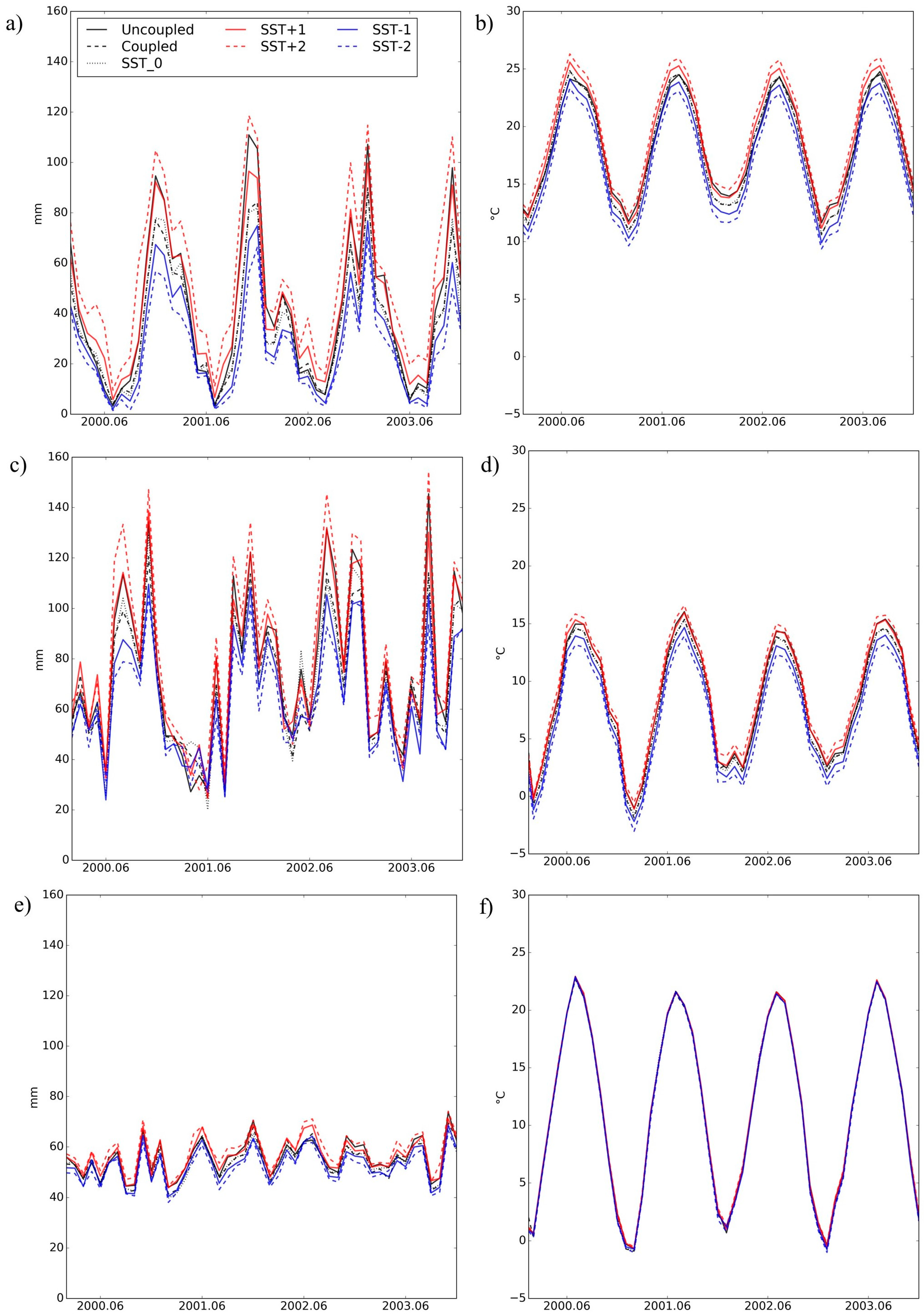
To analyze the changes in the sensitivity experiments, we investigate the time evolution of the field means for precipitation and 2 m temperature over the Mediterranean Sea, the North and Baltic Seas and over the continental areas (Figure 2). The changes are bigger over the seas than over land, which is expected, since we altered one important variable in the air-see interaction process. Nevertheless, we found that over land precipitation is more sensitive to the SST changes than the 2 m temperature, which shows very subtle differences in the sensitivity experiments. The changes in the precipitation and 2 m temperature fields are directly proportional to the SST values, when the SST values rise (decrease), the precipitation and 2 m temperature rises (decreases). Thus, they prove that our assumptions regarding the connection between SST and precipitation and 2 m temperature were right. It is also worth mentioning that the precipitation and 2 m temperature values are not identical in the coupled and in the SST_0 sensitivity experiment, which is the experiment where the uncoupled model uses the six hourly SST results from the coupled simulation. This means, that in the coupled simulation, the two-way interaction between atmosphere and ocean, and the frequent, three hourly coupling has an effect on the simulation. The results from the SST + 1 experiment are close to the results from the uncoupled simulation, which is in accordance with the warmer SST values in Reference [19]. In our previous analysis, we found that the annual mean SST values are on average a 0.5K warmer in the uncoupled simulation compared to the coupled.
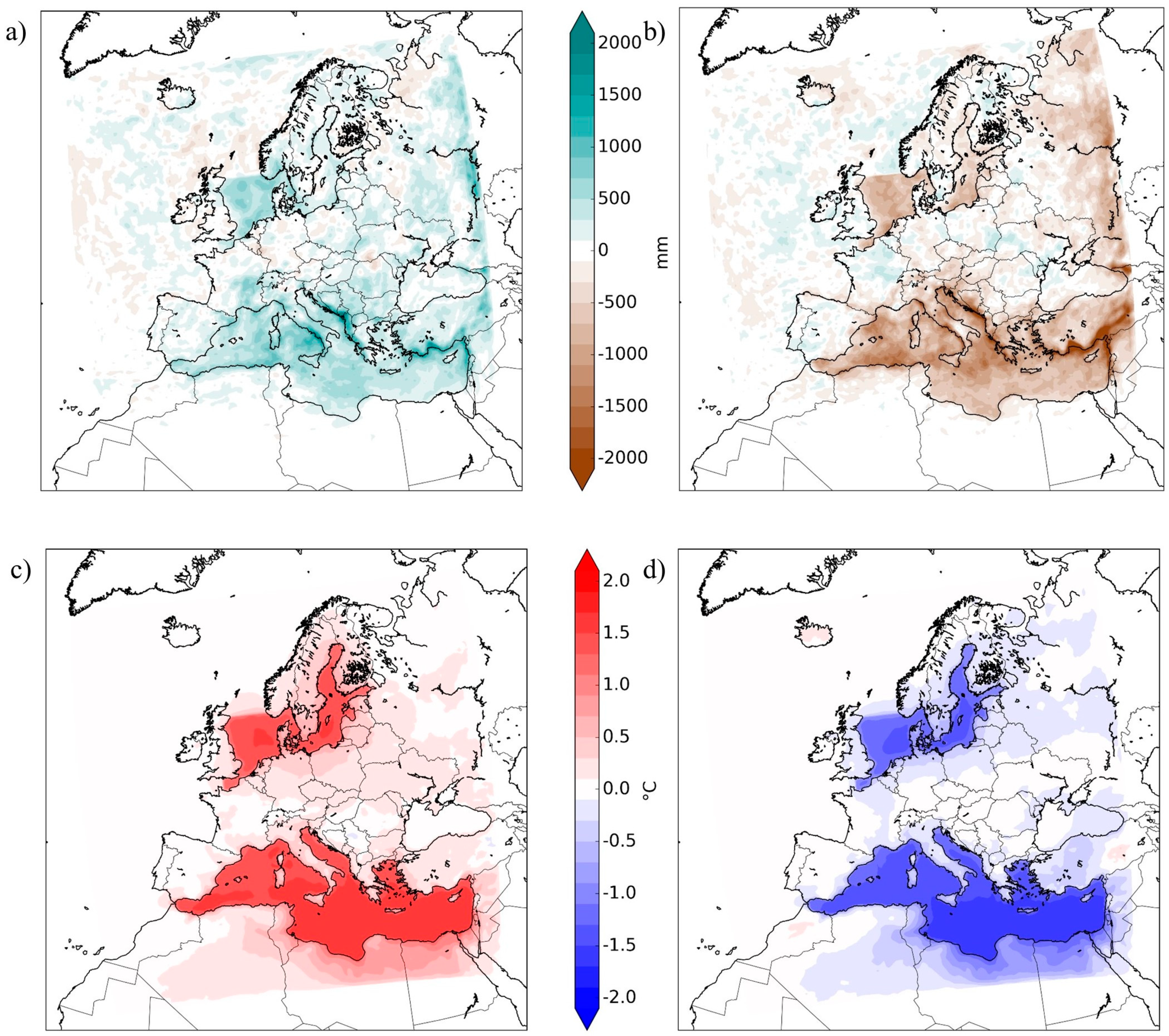
To analyze the pattern of SST sensitivity of precipitation and 2 m temperature, we show the spatial difference between the SST_0 and the two extreme sensitivity experiments (SST – 2 and SST + 2) (Figure 3). The difference between land and sea regions is the most prominent feature of the maps, but in addition, there are also differences along the coastlines. In the case of the 2 m temperature, the magnitude of the difference over the sea is higher than over land, while for precipitation the difference is a bit more homogeneous. The 2 m air temperature’s answer to the +/−2K SST change over the seas are, on average, between 1.1–1.5 K, while over land it is around 0.2 K. In the case of precipitation, the changes over the Mediterranean and the North and Baltic Seas are around 8–19 mm, which is an 11–56% change on average, while over land the change is only 3–4 mm representing 5–8% of the average spatial mean.
Our conclusion is that the atmosphere’s reaction to SST changes, during this short time period, are mostly seen along the coastal regions, and the continental region precipitation has larger variability, due to the change in SST than the 2 m temperature.
The sensitivity experiments give us an estimate regarding the changes one can expect from the coupled simulation, where the dynamically calculated SST is different from the prescribed one in the range of 0.5–1 degrees. The changes in precipitation and 2 m temperature both over land and over the sea are expected to be directly proportional to the change in SST. We expect more changes over land from precipitation than from 2 m temperature, the change in 2 m temperature are expected to be localized to the sea and to the coasts. Nevertheless, online coupling has one big advantage compared to these SST experiments, which is the interaction between the two spheres. Although we cannot quantify this advantage with these sensitivity experiments.

4.2. Precipitation

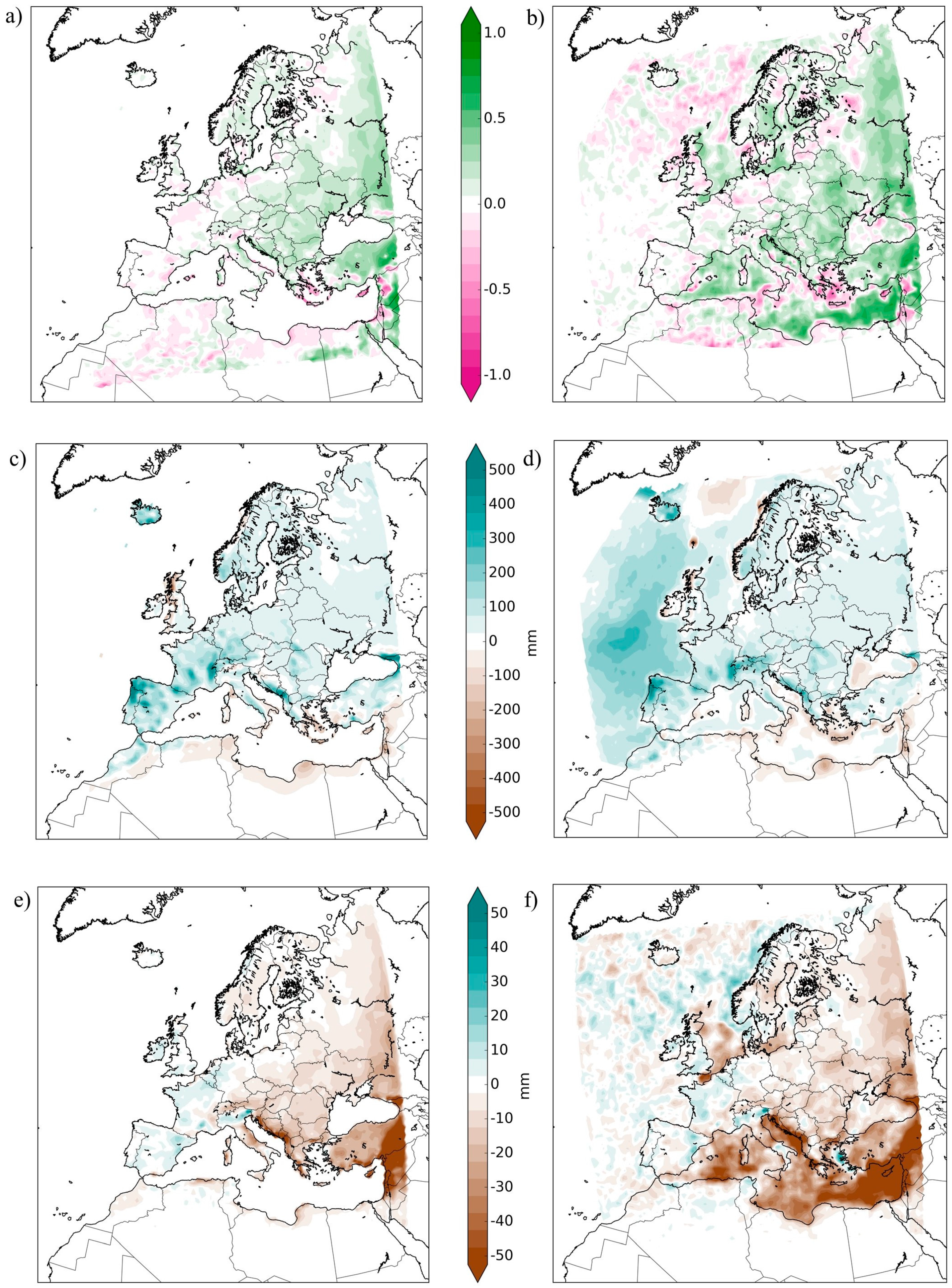
In this sub-section, we analyze the skill scores of the coupled system with regard to precipitation. We evaluated the MSESS of the seasonal precipitation sums of the coupled simulation compared to the uncoupled simulation and found a mostly positive and homogenous skill during winter (Figure 4a,b). The skill during summer (not shown) has a patchy pattern, probably due to the stochastic nature of convective precipitation. The autumn and spring patterns show similarities either to the winter or the summer patterns, respectively. Henceforth, we will focus on the winter precipitation, and to be able to have a broader perspective, we decided to include the MSESS values regarding the HOAPS/GPCC observational dataset, which is available also over marine areas in contrast to the CRU dataset, which is land only. Note, that the CRU dataset contains the whole century, while the HOAPS/GPCC is only available between 1988 and 2008.
The winter MSESS pattern shows positive skill over the coupled seas and also over the area south from a line crossing Europe diagonally from southwest to northeast. This area is downward from the marginal seas, since the circulation in Europe is mainly westerly. To analyze the reason for the positive skill, we analyzed the bias of the coupled system concerning the observations and also the difference between the coupled and uncoupled simulations (Figure 4). We found that the coupled system (Figure 4c,d) and also CCLM alone (not shown) has a wet bias during the winter season over Europe. This wet bias is shown to be reduced by the coupling over the area of the positive skill. Thus, one can conclude that the positive skill is due to the milder overestimation of the precipitation. We compared the median and mean values of seasonal precipitation sums in the coupled and uncoupled simulations to evaluate, whether the difference between the two simulations’ mean seasonal precipitation sums comes from the change of the mean of the distribution or from a shift towards extremes. The two values were very similar—thus, the coupled simulation is on average dryer than the uncoupled simulation. The reduction in the precipitation compared to the uncoupled simulation is probably related to the colder SST values in the coupled seas. We saw by the sensitivity experiments that lower SST values caused less precipitation, mostly over the coupled seas, but also over land. This explains the skill over the seas (Figure 4b), given the wet bias of CCLM during winter.
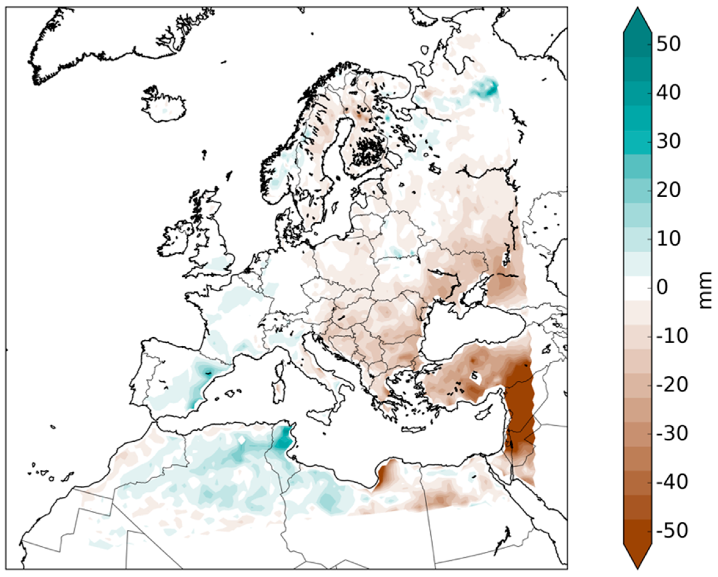
Nevertheless, the results over land are not so explicitly explained by the cooler SST. When comparing the MSESS and difference fields to the sensitivity experiments’ pattern, one sees here more widespread differences over land than at the sensitivity experiments. This is probably in relation to the length of the simulations (110-year-long hindcast versus four-year-long sensitivity studies). During the century-long simulation, the atmosphere and the ocean have more opportunity to interact and represent slow processes. One of such processes is a positive feedback mechanism between precipitation and soil moisture, which helps to propagate the dryer conditions over the continental regions. Figure 5 shows the winter soil moisture content difference between the coupled and the uncoupled simulations, and its pattern mostly coincide with the drier precipitation pattern.
Cooler SST in the coupled simulation during winter, causes less precipitation through the less intense surface fluxes, resulting in dryer soil conditions over land areas downwind from the sea. This decreases evapotranspiration and through that, further decreases precipitation (Figure 6). This feedback mechanism either slows down or intensifies the hydrological cycle. Overall one can see the effect of SST over continental regions, because water vapor does not fall out instantaneously from the air masses; thus, the effect of SST can travel with the circulation, and the feedback mechanism with soil intensifies the signal.

4.3. 2 m Temperature

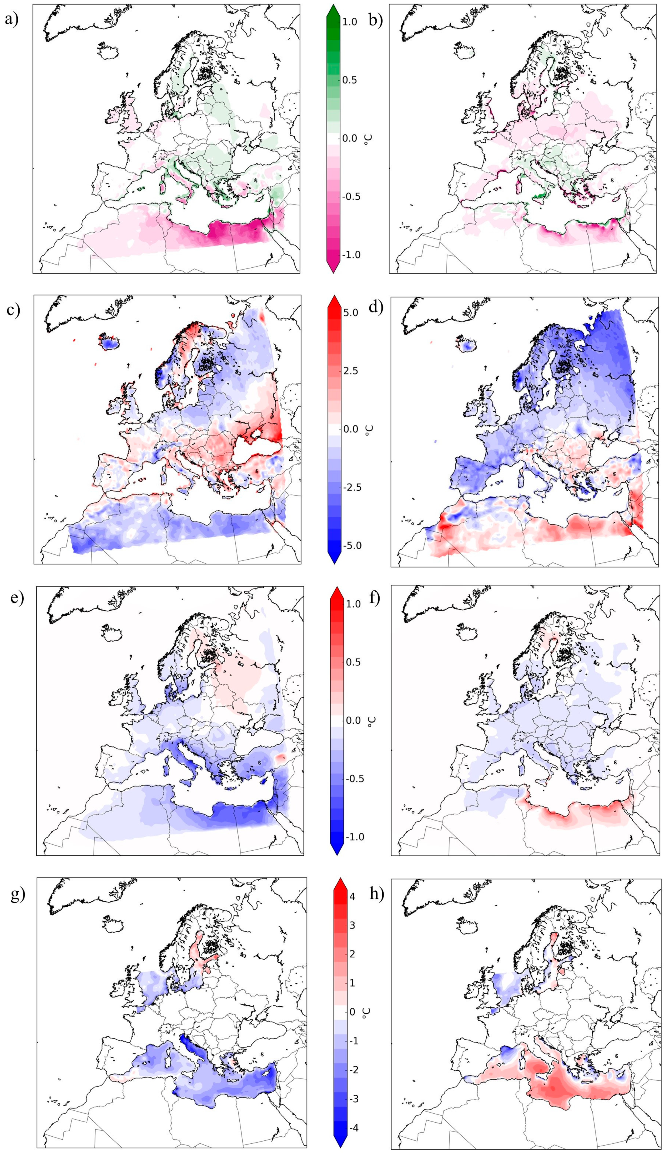
The seasonal analysis of 2 m temperature shows smaller differences between coupled and uncoupled and also less added value compared to the precipitation results (Figure 7). This fits into our expectations based on the sensitivity studies. We include here the 2 m temperature results for the sake of completeness, but one shall note that the differences presented here are so mild that we do not consider them as main results. We present the results for summer and winter, because the spring and autumn patterns can be described as the transitions between these two seasons. Slight positive skill is shown over the Balkan region and along the Italian Peninsula both in winter and summer. Some skill also arises over Scandinavia mainly during the winter period. The difference maps show that the skill over the southern part of Europe is coming from that region’s warm bias being reduced in the coupled simulation. This also applies for the skill over Scandinavia during winter. On the other hand, the reason behind the skill over Scandinavia during summer is that CCLM’s cold bias became warmer via the coupling. Nevertheless, the differences between the coupled and the uncoupled simulation are small, between ±0.5 K. Large negative skill is found over North Africa during winter and to a lesser extent during summer. This is related to the cold (winter) and warm (summer) SST bias near to that coast. Note that although there is a difference between the coupled and the uncoupled simulation in this area, we handle the MSESS values with caution, since this is the area where the CRU dataset has the least stations contributing to the data in our domain.

5. Discussion and Conclusions

The objective of this study was to analyze the added value of coupling regional ocean models to a regional climate model. We evaluated the results from the atmospheric point of view, focusing on results over land and on standard climate variables, such as precipitation and 2 m temperature. The simulation is a hindcast simulation covering the twentieth century, calculated by a coupled system of CCLM for the atmosphere, NEMO-MED12 for the Mediterranean Sea and NEMO-NORDIC for the Baltic and North Seas. Our interest was to find out whether the more detailed background of the regional ocean model, translates into any added value in the atmospheric variables.
To be able to asses CCLM’s reaction to controlled SST changes, we executed some sensitivity experiments with the uncoupled system using altered SST values over the “coupled” seas. As expected, these short (4 year-long) simulations show more sensitivity over the sea. They also showed that with SST decrease, both precipitation and 2 m temperature decrease, due to the changes in surface fluxes, and with SST increase the changes point to the opposite direction. When focusing on land areas, differences due to the SST changes are bigger in the case of precipitation than in the case of 2 m temperature. Thus, we expected a larger effect for precipitation in the coupled simulation. This is indeed what was found in the seasonal analysis. On the seasonal scale for 2 m temperature, we did not find notable changes in the skill over Europe. On the other hand, when using daily data [19] found that in Germany, the coupled simulation is more skillful than the uncoupled, in terms of temperature extremes. Regarding the seasonal precipitation sums, the results show added value, especially during winter over the eastern part of the domain.
During summer the pattern of MSESS are relatively patchy compared to the winter results. This is probably due to the different mechanisms driving the precipitation formation. First of all, summer precipitation contains more convective events, which have a stochastic characteristic, and those could be responsible for the patchiness of the skill. Moreover, CCLM’s precipitation bias is not homogenously wet over whole of Europe during summer as it is during winter. It has even dry regions (e.g., the Balkans and Eastern Europe). Moreover, the coupled system’s SST bias over the Mediterranean Sea differs during summer and winter. In winter, it is cooler than observations, while in summer, it is not colder, but even warmer over some regions [19]. Thus, the drying effect of the cold SST, which is responsible for the winter skill presented in Section 4, does not act during the summer periods, and other processes do not seem to improve the summer results.
The added skill during winter is associated with dryer conditions in the coupled simulation, which means the wet bias of CCLM is improved by the coupling. This is in accordance with the simulated SST values, which are on average cooler than the SST boundary conditions used in the uncoupled simulation. The sensitivity experiments also showed us, that the cooler the SST, the dryer the model. Thus, in the coupled simulation, the cooler SST values induce less precipitation, which partially corrects the overestimation of precipitation. Moreover, the added skill was found not just around the coastlines, but over areas, with a more continental climate. The lack of precipitation in the coupled simulation causes dryer soil conditions, which furthermore decreases precipitation, through a positive feedback mechanism [36]. Additionally, when one compares the pattern from the SST + 2 experiment (Figure 3b) and the difference between the coupled and uncoupled simulation (Figure 4e,f) one sees more elaborate changes in the hindcast simulation. This suggests, that the longer the time period, the more widespread the differences between the coupled and the uncoupled run. Hence, differences are connected to those parts of the system that have a longer memory, such as the soil or the seas. The importance of these parts increases in long term projections. This finding contradicts the findings of References [21] and [37], who found that coupling regional oceans do not have far-reaching effects over the continental atmospheric variables. Nevertheless, the mentioned studies considered several decade-long coupled simulations, which is significantly shorter than our century-long simulation. Moreover, they included less sea area in the coupling. Reference [21] coupled the North and Baltic Seas and [37] only the Mediterranean Sea, not all three marginal seas as our study did. On the other hand, Reference [5] found that in their coupled simulation with CCLM and NEMO-NORDIC, coupling affected the eastern part of the domain. Although they investigated 2 m temperature and found the largest differences during summer. We found the eastern European pattern during winter and in the case of precipitation. Nevertheless, this can also suggest that the changes in the eastern part of the domain might be a CCLM-NEMO specific feature.
The fact that the added skill in the coupled simulation is due to the lack of precipitation is somewhat similar to the findings of Reference [37], who found that in their high resolution coupled simulation, the representation of hot days and droughts improved more than the representation of heavy precipitation events. They concluded that the improvement of hot days and droughts, which are mostly driven at synoptic scales, is due to the better representation of topography and local processes, while they suggest that the lack of improvement in heavy precipitation might be due to the inaccurate tuning of the parameters at high resolution. This might also be the case in our system, since we see some inconsistency regarding the fact that the coupled system has even bigger SST bias than the uncoupled system [19], and yet the coupled system’s precipitation bias decreases.
Therefore, regarding the coupled system, we conclude that it performs at some aspects better and at least, as well as the uncoupled system. This is already a great success, given that the coupled system is more complex and has more degrees of freedom to develop its own stable state. Therefore, if it is closer to reality, it is a more reliable system than an uncoupled model, and can be used for future assessments as well. Moreover, our simulation proves that the correct representation of slow systems with a long memory, is increasingly important, when considering century-long simulations. To summarize the results, we answer the main research questions of this study:
  • How sensitive is the atmosphere, namely the precipitation and 2 m temperature, to SST changes in the model system?
    Based on our sensitivity experiments with altered SST values, we conclude that both precipitation and 2 m temperature react to SST changes. The changes are mostly over the sea areas, but some differences appear over land as well. Additionally, over continental areas precipitation seems to be more affected than 2 m temperature.
  • Has the interactive coupling of atmosphere and ocean an effect over the continental areas?
    Yes, it has. As expected from the sensitivity experiments, precipitation is influenced by the coupling. Nevertheless, it is unclear if the difference over continental regions is due to the model’s specific feature or the result of the length of the simulation, since the century-long simulation enables the slow parts of the system to evolve and show their effect on the results. This is also an important finding to prove the importance of marginal seas further away from the coasts.
  • Is there any large scale added skill in the precipitation and in the 2 m temperature variables in the coupled simulation compared to the uncoupled one?
    Yes, during winter the precipitation has positive skill over the eastern part of the domain. We found that the coupled system has in average a bit colder SST values than the atmosphere-only version. This leads to less precipitation, meaning smaller wet bias during winter over the eastern part of the domain. This, together with a soil moisture-evapotranspiration-precipitation positive feedback loop results in a homogenous increase in skill over a large area. In terms of 2 m temperature, we found only moderate skill in Europe.
The results showed added value, due to coupling, but there are still open questions to be answered. The hydrological cycle in the coupled system needs further evaluation and possibly tuning, since the presented added value in winter precipitation is partly due to counteracting biases. Based on our results, we assume that one possible way for improving the atmospheric model’s physics would be to revise the parametrization governing the surface fluxes over the sea. The biases of the ocean model (e.g., the SST biases) also need to be investigated. It is also worth mentioning that closing the water budget with a runoff model is already in progress for our coupled set up. The comparison with other century-long coupled simulations could also help to determine the source of the added value over the continental regions.

Author Contributions

In this research article the authors contribution as follows: Conceptualization, F.D.K. and B.A.; methodology, F.D.K.; software, C.P. and H.F.; validation, F.D.K. and C.P.; formal analysis, F.D.K.; investigation, F.D.K.; resources, B.A.; data curation, C.P. and H.F.; writing—original draft preparation, F.D.K.; writing—review and editing, F.D.K., C.P., B.A., H.F.; visualization, F.D.K.; supervision, B.A.; project administration, B.A. and H.F.; funding acquisition, B.A.

Funding

This research received founding from the German Federal Ministry of Education and Research (BMBF) under Grant MiKlip: FKZ01LP1518C/A and from the German Research Foundation (“Deutsche Forschungsgemeinschaft”, DFG) in terms of the research group FOR 2416 “Space-Time Dynamics of Extreme Floods (SPATE)”, and funding from the European Union’s Horizon 2020 research and innovation programme under grant agreement No 776661, entitled DownScaling CLImate ImPACTs and decarbonisation pathways in EU islands, and enhancing socioeconomic and non-market evaluation of Climate Change for Europe, for 2050 and Beyond.

Acknowledgments

The authors acknowledge support by the German Federal Ministry of Education and Research (BMBF) under Grant MiKlip: FKZ01LP1518C/A, the German Research Foundation (“Deutsche Forschungsgemeinschaft”, DFG) in terms of the research group FOR 2416 “Space-Time Dynamics of Extreme Floods (SPATE)”and funding from the European Union’s Horizon 2020 research and innovation programme under grant agreement No 776661, entitled DownScaling CLImate ImPACTs and decarbonisation pathways in EU islands, and enhancing socioeconomic and non-market evaluation of Climate Change for Europe, for 2050 and Beyond. The opinions expressed are those of the author(s) only and should not be considered as representative of the European Commission’s official position. The authors also thank the Centre for Scientific Computing (CSC) of the Goethe University Frankfurt and the German High-Performance Computing Centre for Climate and Earth System Research (“Deutsches Klimarechenzentrum”, DKRZ) for supporting the calculations. Special thanks to Christian Dieterich and other colleagues from SMHI for providing the NEMO-NORDIC model and to Naveed Akhtar from HZG for helping with the coupled set-up. We thank both reviewers, whose constructive comments helped to improve the manuscript.

Conflicts of Interest

The authors declare no conflict of interest.

References

  1. Giorgi, F.; Mearns, L.O. Approaches to the simulation of regional climate change: A review. Rev. Geophys. 1991, 29, 191–216. [Google Scholar] [CrossRef]
  2. Feser, F.; Rrockel, B.; Storch, H.; Winterfeldt, J.; Zahn, M. Regional climate models add value to global model data a review and selected examples. Bull. Am. Meteorol. Soc. 2011, 92, 1181–1192. [Google Scholar] [CrossRef]
  3. Li, L.; Bozec, A.; Somot, S.; Beranger, K.; Bouruet-Aubertot, P.; Sevault, F.; Crepon, M. Regional atmospheric, marine processes and climate modelling. In Mediterranean Climate Variability; Lionello, P., Malanotte, R., Eds.; Elsevier B.V: Amsterdam, The Netherlands, 2006; pp. 373–397. [Google Scholar]
  4. Somot, S.; Sevault, F.; Déqué, M.; Crépon, M. 21st century climate change scenario for the Mediterranean using a coupled atmosphere-ocean regional climate model. Glob. Planet. Change 2008, 63, 112–126. [Google Scholar] [CrossRef]
  5. Van Pham, T.; Brauch, J.; Dieterich, C.; Frueh, B.; Ahrens, B. New coupled atmosphere-ocean-ice system COSMO-CLM/NEMO: Assessing air temperature sensitivity over the North and Baltic Seas. Oceanologia 2014, 56, 167–189. [Google Scholar] [CrossRef]
  6. Rinke, A.; Gerdes, R.; Dethloff, K.; Kandlbinder, T.; Karcher, M.; Kauker, F.; Frickenhaus, S.; Köberle, C.; Hiller, W. A case study of the anomalous Arctic sea ice conditions during 1990: Insights from coupled and uncoupled regional climate model simulations. J. Geophys. Res. Atmos. 2003, 108, 4275. [Google Scholar] [CrossRef]
  7. Akhtar, N.; Brauch, J.; Dobler, A.; Béranger, K.; Ahrens, B. Medicanes in an ocean-atmosphere coupled regional climate model. Nat. Hazards Earth Syst. Sci. 2014, 14, 2189–2201. [Google Scholar] [CrossRef]
  8. Giorgi, F. Climate change hot-spots. Geophys. Res. Lett. 2006, 33, 1–4. [Google Scholar] [CrossRef]
  9. Artale, V.; Calmanti, S.; Carillo, A.; Dell’Aquila, A.; Herrmann, M.; Pisacane, G.; Ruti, P.M.; Sannino, G.; Struglia, M.V.; Giorgi, F.; et al. An atmosphere-ocean regional climate model for the Mediterranean area: Assessment of a present climate simulation. Clim. Dyn. 2010, 35, 721–740. [Google Scholar] [CrossRef]
  10. Drobinski, P.; Anav, A.; Brossier, C.L.; Samson, G.; Stéfanon, M.; Bastin, S.; Baklouti, M.; Béranger, K.; Beuvier, J.; Bourdallé-Badie, R.; et al. Model of the Regional Coupled Earth system (MORCE): Application to process and climate studies in vulnerable regions. Environ. Model. Softw. 2012, 35, 1–18. [Google Scholar] [CrossRef]
  11. Lebeaupin Brossier, C.; Drobinski, P.; Béranger, K.; Bastin, S.; Orain, F. Ocean memory effect on the dynamics of coastal heavy precipitation preceded by a mistral event in the northwestern Mediterranean. Q. J. R. Meteorol. Soc. 2013, 139, 1583–1597. [Google Scholar] [CrossRef]
  12. Lebeaupin Brossier, C.; Béranger, K.; Deltel, C.; Drobinski, P. The Mediterranean response to different space-time resolution atmospheric forcings using perpetual mode sensitivity simulations. Ocean Model. 2011, 36, 1–25. [Google Scholar] [CrossRef]
  13. Sevault, F.; Somot, S.; Alias, A.; Dubois, C.; Lebeaupin-Brossier, C.; Nabat, P.; Adloff, F.; Déqué, M.; Decharme, B. A fully coupled Mediterranean regional climate system model: design and evaluation of the ocean component for the 1980–2012 period. Tellus A Dyn. Meteorol. Oceanogr. 2014, 66, 23967. [Google Scholar] [CrossRef]
  14. Döös, K.; Meier, H.E.M.; Döscher, R. The Baltic Haline Conveyor Belt or The Overturning Circulation and Mixing in the Baltic. AMBIO A J. Hum. Environ. 2009, 33, 261–266. [Google Scholar] [CrossRef]
  15. Daewel, U.; Schrum, C. Simulating long-term dynamics of the coupled North Sea and Baltic Sea ecosystem with ECOSMO II: Model description and validation. J. Mar. Syst. 2013, 119–120, 30–49. [Google Scholar] [CrossRef]
  16. Schrum, C.; Hübner, U.; Jacob, D.; Podzun, R. A coupled atmosphere/ice/ocean model for the North Sea and the Baltic Sea. Clim. Dyn. 2003, 21, 131–151. [Google Scholar] [CrossRef]
  17. Doscher, R.; Willén, U.; Jones, C.; Rutgersson, A.; Meier, H.M.; Hansson, U.; Graham, L.P. The development of the regional coupled ocean-atmosphere model RCAO. Boreal Environ. Res. 2002, 7, 183–192. [Google Scholar]
  18. Dieterich, C.; Wang, S.; Schimanke, S.; Gröger, M.; Klein, B.; Hordoir, R.; Samuelsson, P.; Liu, Y.; Axell, L.; Höglund, A.; et al. Surface Heat Budget over the North Sea in Climate Change Simulations. Atmosphere (Basel). 2019, 10, 272. [Google Scholar] [CrossRef]
  19. Primo, C.; Kelemen, F.D.; Feldmann, H.; Ahrens, B. A regional atmosphere-ocean climate system model over Europe including three marginal seas: On its stability and performance. Geosci. Model Dev. 2019, 1–33. [Google Scholar] [CrossRef]
  20. Akhtar, N.; Brauch, J.; Ahrens, B. Climate modeling over the Mediterranean Sea: impact of resolution and ocean coupling. Clim. Dyn. 2018, 51, 933–948. [Google Scholar] [CrossRef]
  21. Gröger, M.; Dieterich, C.; Meier, M.H.E.; Schimanke, S. Thermal air-sea coupling in hindcast simulations for the North Sea and Baltic Sea on the NW European shelf. Tellus Ser. A Dyn. Meteorol. Oceanogr. 2015, 67, 1. [Google Scholar] [CrossRef]
  22. Rockel, B.; Castro, C.L.; Pielke, R.A.; von Storch, H.; Leoncini, G. Dynamical downscaling: Assessment of model system dependent retained and added variability for two different regional climate models. J. Geophys. Res. 2008, 113, 1–9. [Google Scholar] [CrossRef]
  23. Doms, G.; Förstner, J.; Heise, E.; Herzog, H.J.; Mironov, D.; Raschendorfer, M.; Reinhardt, T.; Ritter, B.; Schrodin, R.; Schulz, J.P.; et al. A Description of the Nonhydrostatic Regional COSMO Model Part II: Physical Parameterization. In Consortium for Small-Scale Modelling; Deutscher Wetterdienst: Offenbach, Germany, 2011; p. 154. [Google Scholar]
  24. Giorgi, F.; Jones, C.; Asrar, G.R. Addressing climate information needs at the regional level: the CORDEX framework. World Meteorol. Organ. Bull. 2009, 58, 175–183. [Google Scholar]
  25. Müller, W.A.; Pohlmann, H.; Sienz, F.; Smith, D. Decadal climatepredictions for theperiod1901–2010 with a coupled climate model. Geophys. Res. Lett. 2014, 41, 2100–2107. [Google Scholar] [CrossRef]
  26. Müller, W.A.; Matei, D.; Bersch, M.; Jungclaus, J.H.; Haak, H.; Lohmann, K.; Compo, G.P.; Sardeshmukh, P.D.; Marotzke, J. A twentieth-century reanalysis forced ocean model to reconstruct the North Atlantic climate variation during the 1920s. Clim. Dyn. 2015, 44, 1935–1955. [Google Scholar] [CrossRef]
  27. Compo, G.P.; Whitaker, J.S.; Sardeshmukh, P.D.; Matsui, N.; Allan, R.J.; Yin, X.; Gleason, B.E.; Vose, R.S.; Rutledge, G.; Bessemoulin, P.; et al. The Twentieth Century Reanalysis Project. Q. J. R. Meteorol. Soc. 2011, 137, 1–28. [Google Scholar] [CrossRef]
  28. Rayner, N.A. Global analyses of sea surface temperature, sea ice, and night marine air temperature since the late nineteenth century. J. Geophys. Res. 2003, 108, 4407. [Google Scholar] [CrossRef]
  29. Beuvier, J.; Brossier, C.L.; Béranger, K.; Arsouze, T.; Bourdallé-Badie, R.; Deltel, C.; Drillet, Y.; Drobinski, P.; Ferry, N.; Lyard, F.; et al. MED12, oceanic component for the modeling of the regional Mediterranean earth system. Mercat. Ocean Q. Newsl. 2012, 46, 60–66. [Google Scholar]
  30. Hordoir, R.; Axell, L.; Höglund, A.; Dieterich, C.; Fransner, F.; Groger, M.; Liu, Y.; Pemberton, P.; Schimanke, S.; Andersson, H.; et al. Nemo-Nordic 1.0: A NEMO-based ocean model for the Baltic and North seas - Research and operational applications. Geosci. Model Dev. 2019, 12, 363–386. [Google Scholar] [CrossRef]
  31. Vancoppenolle, M.; Fichefet, T.; Goosse, H.; Bouillon, S.; Madec, G.; Maqueda, M.A.M. Simulating the mass balance and salinity of Arctic and Antarctic sea ice. 1. Model description and validation. Ocean Model. 2009, 27, 33–53. [Google Scholar] [CrossRef]
  32. Craig, A.; Valcke, S.; Coquart, L. Development and performance of a new version of the OASIS coupler, OASIS3-MCT-3.0. Geosci. Model Dev. 2017, 10, 3297–3308. [Google Scholar] [CrossRef]
  33. Harris, I.; Jones, P.D.; Osborn, T.J.; Lister, D.H. Updated high-resolution grids of monthly climatic observations - the CRU TS3.10 Dataset. Int. J. Climatol. 2014, 34, 623–642. [Google Scholar] [CrossRef]
  34. Andersson, A.; Ziese, M.; Dietzsch, F.; Schröder, M.; Becker, A.; Schamm, K. HOAPS/GPCC European daily precipitation data record with uncertainty estimates using satellite and gauge based observations at 0.5°. Glob. Precip. Climatol. Cent. Dtsch. Wetterd. 2016. [Google Scholar] [CrossRef]
  35. Murphy, A.H. Skill scores based on the mean square error and their relationships to the correlation coefficient. Mon. Weather Rev. 1988, 116, 2417–2424. [Google Scholar] [CrossRef]
  36. Schär, C.; Lüthi, D.; Beyerle, U.; Heise, E. The soil-precipitation feedback: A process study with a regional climate model. J. Clim. 1999, 12, 722–741. [Google Scholar] [CrossRef]
  37. Panthou, G.; Vrac, M.; Drobinski, P.; Bastin, S.; Li, L. Impact of model resolution and Mediterranean sea coupling on hydrometeorological extremes in RCMs in the frame of HyMeX and MED-CORDEX. Clim. Dyn. 2018, 51, 915–932. [Google Scholar] [CrossRef]
Figure 1. Connection between SST (seas surface temperature), and precipitation and 2 m temperature.
Atmosphere 10 00537 g001
Figure 2. Time evolution (2000–2003) of precipitation (left column) and 2 m temperature (right column) field mean over the Mediterranean Sea (a,b), the Baltic and the North Seas (c,d) and over land (e,f) in the sensitivity experiments and in the coupled and uncoupled simulation.
Atmosphere 10 00537 g002
Figure 3. Difference between the SST_0 and the SST – 2 (left column, a,c) or the SST + 2 (right column, b,d) simulations. The first row (a,b) shows the difference of the precipitation sums during the whole time period (2000–2003) and the second row (c,d) shows the differences in 2 m temperature mean.
Atmosphere 10 00537 g003
Figure 4. Mean winter precipitation sum: (a) Mean square error skill score (MSESS) values comparing the coupled system to the uncoupled with respect to CRU (Climatic Research Unit) (1901–2009) and (b) with respect to HOAPS/GPCC (Hamburg Ocean Atmosphere Parameters and Fluxes from Satellite Data, Global Precipitation Climatology Centre) (1988–2008), (c) bias of the coupled system with respect to CRU and (d) HOAPS/GPCC, (e) difference between the coupled and the uncoupled system for the time period 1901–2009 and for (f) 1988–2008.
Atmosphere 10 00537 g004
Figure 5. The difference of mean soil moisture content during winter between the coupled and the uncoupled simulation.
Atmosphere 10 00537 g005
Figure 6. Positive feedback mechanism between precipitation, soil moisture and evapotranspiration.
Atmosphere 10 00537 g006
Figure 7. Winter (left column) and summer (right column) mean 2 m air temperature (a,b) MSESS (c,d) bias compared to CRU data and (e,f) difference between coupled and uncoupled simulation. (g,h) Seasonal mean SST difference between coupled and uncoupled simulation.
Atmosphere 10 00537 g007
Table 1. Summary of the simulations compared in the sensitivity study. CCLM (Consortium for Small-Scale Modeling, Climate Limited-area Model), NEMO (Nucleus for European Modelling of the Ocean), CPL (coupled simulation, CCLM-NEMO).
Experiment NameUncoupledCoupledSST_0SST + 1SST – 1SST + 2SST – 2
ModelCCLMCCLM-NEMOCCLMCCLMCCLMCCLMCCLM
SST
(marginal seas)
MPI-ESM-LR as20ncep08SST from NEMO
(CPL SST)
CPL SSTCPL SST + 1CPL SST – 1CPL SST + 2CPL SST – 2