Article

Multiscale Spatio-Temporal Changes of Precipitation Extremes in Beijing-Tianjin-Hebei Region, China during 1958–2017

1
School of Resources and Geosciences, China University of Mining & Technology, Xuzhou 221116, China
2
State Key Laboratory of Hydrology-Water Resources and Hydraulic Engineering, Nanjing Hydraulic Research Institute, Nanjing 210029, China
3
State Key Laboratory of Water Resources and Hydropower Engineering Science, Wuhan University, Wuhan 430072, China
*
Author to whom correspondence should be addressed.
Atmosphere 2019, 10(8), 462; https://doi.org/10.3390/atmos10080462
Submission received: 12 June 2019 / Revised: 29 July 2019 / Accepted: 10 August 2019 / Published: 13 August 2019
(This article belongs to the Section Meteorology)

Abstract

:
In this study, based on daily precipitation records during 1958–2017 from 28 meteorological stations in the Beijing-Tianjin-Hebei (BTH) region, the spatio-temporal variations in precipitation extremes defined by twelve indices are analyzed by the methods of linear regression, Mann-Kendall test and continuous wavelet transform. The results showed that the spatial patterns of all the indices except for consecutive dry days (CDD) and consecutive wet days (CWD) were similar to that of annual total precipitation with the high values in the east and the low value in the west. Regionally averaged precipitation extremes were characterized by decreasing trends, of which five indices (i.e., very heavy precipitation days (R50), very wet precipitation (R95p), extreme wet precipitation (R99p), max one-day precipitation (R × 1day), and max five-day precipitation (R × 5day)) exhibited significantly decreasing trends at 5% level. From monthly and seasonal scale, almost all of the highest values in R × 1day and R × 5day occurred in summer, especially in July and August due to the impacts of East Asian monsoon climate on inter-annual uneven distribution of precipitation. The significant decreasing trends in annual R×1day and R×5day were mainly caused by the significant descend in summer. Besides, the possible associations between precipitation extremes and large-scale climate anomalies (e.g., ENSO (El Niño Southern Oscillation), NAO (North Atlantic Oscillation), IOD (Indian Ocean Dipole), and PDO (Pacific Decadal Oscillation)) were also investigated using the correlation analysis. The results showed that the precipitation extremes were significantly influenced by ENSO with one-year ahead, and the converse correlations between the precipitation extremes and climate indices with one-year ahead and 0-year ahead were observed. Moreover, all the indices show significant two- to four-year periodic oscillation during the entire period of 1958–2017, and most of indices show significant four- to eight-year periodic oscillation during certain periods. The influences of climate anomalies on precipitation extremes were composed by different periodic components, with most of higher correlations occurring in low-frequency components.

1. Introduction

With the global hydrological cycle accelerating subsequently in the background of climate warming [1], extreme climate events have become more frequent [2], which has a significant impact on human society and even causes serious losses to people’s lives and property [3,4,5]. Correspondingly, extreme events and related societal impacts are becoming an increasingly interesting area and has also attracted great attention, especially in the field of meteorology [6]. The Expert Team on Climate Change Detection and Indices (ETCCDI) has defined a set of climate indices to provide the widespread overview of daily temperature and precipitation. These extreme indices have been widely used all around the world for analyzing the changes in extreme in the past as well as in the future [7,8,9].
Because natural disasters associated with precipitation extremes have greater widespread impact on human society and economy, understanding the variation in precipitation extremes is important for protecting the safety of water resources, terrestrial ecosystems, and eventually the sustainability of human society [10]. Therefore, given the potentially significant social, economic, and ecological impacts of extreme precipitation events, comprehensive and up-to-date assessments of precipitation extremes at a local scale are beneficial for water resources management, flood control, and prevention under a changing environment. Previous studies investigated trends and variability of precipitation extremes in many parts of the world. On a global scale, the changes in precipitation extremes have a complicated pattern and have apparent regional characteristics [11,12], with the largest changes in the tropics [13]. Increasing precipitation extremes are shown in large areas, but the spatio-temporal patterns of precipitation extremes are much more complicated than for temperature extremes. On regional scales, many studies on precipitation extremes have emerged in recent years [14,15,16,17,18,19,20], and the results have also shown small spatial coherence. For example, over North America, there has been a sizable increase in the frequency of extreme precipitation events since the 1920s/1930s in the U.S. whereas there has been no discernible trend in the frequency of the most extreme events in Canada [21]. For South America, the pattern of trends for extreme precipitation is generally the same as that for total annual rainfall, with most parts of this region increasing since 1960s [22]. In Europe, significant increasing trends in annual precipitation extremes have been detected in different regions [23,24]. The extreme precipitation events in western African and western Indian regions have shown a descending trend since the middle of the last century [25,26]. In China, on average, the frequency and intensity of extreme precipitation events have increased, and they show apparent spatial differences [6,27,28,29], with the positive trends occurring in the Yangtze River basin, southeastern China, and northwestern China, while the negative trends existing in the Yellow River basin, northern China, and central Tibetan Plateau [30,31,32]. These results highlight the tendencies and characteristics of extreme precipitation events in different regions [33], showing that the long-term temporal trends of extreme precipitation have varied regionally around the world, indicating the importance of more localized studies [34,35].
In the context of global warming, the effects of extreme events on economic and social development have exacerbated in China. This is particularly true for those urban agglomeration areas, such as Beijing-Tianjin-Hebei (BTH), Yangtze River Delta, and Pearl River Delta urban agglomerations. The BTH region is one of the most important economic, political, cultural, and transportation centers in China, and is becoming more and more important in the world encouraged by the coordinated development of BTH. Recently, more and more extreme events are reported in this region, such as the severe drought in Tianjin during 1980–1982, the continuous high temperature event over Beijing in the early July 2010, and the extraordinary rainstorm disaster in Beijing in 2004, 2011, 2012, and 2016, and so on. Therefore, a comprehensive understanding of changes in extreme precipitation in this area would be helpful for the regional disaster prevention and mitigation, and sustainable development. Previous studies have reported that extreme precipitation has changed over the past few decades in this region or neighboring regions (e.g., North China, Haihe River basin). For example, Mei et al. [33] analyzed the spatial and temporal changes in extreme precipitation in this region based on the ETCCDI indices and 26 meteorological station data during 1960–2013, and found the indices of R × 1day and R × 5day showed significantly decreasing trend and there were visible spatial variations of all the indices influenced by the spatial distribution of terrain. Zhang et al. [36] discussed the nonstationary of extreme precipitation over the BTH region with Generalized Additive Models for Location, Scale, and Shape (GAMLSS) method using the annual maximum daily precipitation series from 12 meteorological stations, and found that maximum daily precipitation in the BTH region also showed a decreasing trend from 1960 to 2013. Wei et al. [37] conducted the recent trends of extreme precipitation in Beijing-Tianjin Sand source region based on 53 stations during 1960–2014, and found most extreme precipitation indices showed an insignificant decreasing trend with exception in R × 1day and R × 5day. Shen et al. [38] summarized the spatial and temporal variations of extreme precipitation over the BTH region using the percentile method and 174 station data during 1981–2016, and they found the spatial patterns of extreme precipitation indices except for extreme precipitation days are similar and extreme precipitation events frequently occurred in July, August, and October. Additionally, for the neighboring regions of BTH, Du et al. [39] reported that alterations in extreme precipitation mainly occurred north of 38° N, and decreasing trends in extreme precipitation were detected at most stations in the Haihe River basin. Zhou et al. [40] reported that all cities in the BTH region showed decline trends in extreme precipitation during 1960–2014, with a significant decreasing trend in megacities based on linear regression method.
Additionally, variations of precipitation extremes are caused by many forcing factors, such as large-scale atmospheric circulation, topography, and local climate [14,32,41,42,43,44,45,46,47,48,49]. For example, Xiao et al. [41] analyzed the teleconnections between precipitation extremes and El Niño Southern Oscillation (ENSO), North Atlantic Oscillation (NAO), Indian Ocean Dipole (IOD), and Pacific Decadal Oscillation (PDO) using the regression method, and found that regional responses of precipitation extremes to climate indices varied at different stages. Chen et al. [42] investigated the possible association between temporal patterns of precipitation extreme over China with large-scale ocean-atmospheric indices (e.g., NAO, PDO, Arctic Oscillation (AO), NINO3 (Niño3 sea surface temperature (SST) index), NINO3.4 (Niño3.4 SST index), and other SST indices) based on grid daily precipitation data during 1963–2013, and found that precipitation extremes in four different seasons were influenced by the different combinations of large-scale climate indices with different time lags, and their regional relations are complex when the climate indices were at different phases. Xue et al. [10] discussed the long-term trends of precipitation extremes and underlying mechanisms in U.S. Great Basin during 1951–2013, and found that the effects of ENSO and PDO on precipitation and precipitation extremes were low, while the intensifying high-pressure system over the western North Pacific in winter and increasing water vapor and air temperature of the atmosphere over the basin in winter and spring were mainly responsible for the upward trends of precipitation extremes. With advances in the field of synoptic climatology, it has been found that ocean-atmosphere interactions are not chaotic or random, it is therefore possible to identify the relationship between ocean-atmospheric modes and hydrological variables. Related studies revealed that the ENSO, PDO, and other large-scale atmospheric circulation are likely to be important factors in the variability of precipitation extremes on both spatial and temporal scales. And these climate anomalies will be helpful for prediction/forecasting of precipitation extremes. However, few efforts have been made on the possible linkage between precipitation extremes over BTH and the large-scale atmospheric circulation. Thus, to better understanding the changes of precipitation extremes, the associations between regional precipitation extremes and large-scale climate anomalies should be further discussed.
Although many researchers have conducted analyses regarding the changes of precipitation extremes, the long-term trends with different scales over the BTH region and the possible teleconnection with large-scale climate anomalies still need to be strengthened. Additionally, assessing the temporal trends and spatial patterns of precipitation extremes in BTH will provide information for managing water resources effectively and better responding the extreme events. Therefore, the main objectives of our study are (1) to investigate the spatial-temporal variability of extreme precipitation at different scales over the BTH region using several trend detecting and periodicity analysis methods based on the 28 meteorological stations during 1958–2017, and (2) to identify the dominant climate factors in explaining extreme precipitation changes by investigating the statistical association between temporal patterns of extreme precipitation signals with large-scale ocean-atmosphere indices using correlation analysis.

2. Materials and Methods

2.1. Study Area

The study area (Figure 1a), which is located in 113°04′–119°53′ E, 36°01′–42°37′ N, has a total area of about 217,185 km2. It includes Beijing municipality, Tianjin municipality, and other 11 cities in Hebei Province (the BTH region), also known as Jing-jin-ji Metropolitan Region or Jing-Jin-Ji (JJJ). As shown in Figure 1c, the spatial pattern of elevation exhibits the obvious feature of “high in the northwest and low in the southeast”. The eastern and southern part of BTH are adjacent to the Yellow River and Bohai Sea, with elevation less than 500 m. Taihang and Yan mountains are in western and northern part of the BTH region, which constitute 53.6% of the total area. The monsoon climate has obvious seasonal variations characterized by hot, rainy summers, and cold, dry winters. Meteorological disasters in this region are frequent and have caused serious damages to human life especially in recent years. Drought often strikes in the spring and flooding occurs in the summer. From the annual precipitation totals, BTH as a whole is commonly regarded as a semi-humid region, with a mean annual total precipitation of 540 mm. Figure 1b showed the spatial distribution of annual mean precipitation over BTH during 1958–2017. The annual mean precipitation increased from the west to the east in the BTH region, ranging from 393 mm to 723.4 mm, with the highest value (Zunhua station (No. 13 in Figure 1)) located in the belt between the mountain and plain areas.

2.2. Data Collection and Processing

2.2.1. Precipitation Data

The daily precipitation dataset [51] of 28 meteorological stations (Table 1 and Figure 1) provided by the China Meteorological Administration (CMA) was used to extract time series of extreme precipitation. The weather stations have a reasonable spatial coverage, consequently being able to emphasize the regional behavior and variability of the precipitation extremes in the BTH region. The geographical coordinates of the stations are shown in Table 1. Before constructing the precipitation indices series, data quality control and homogeneity assessment were performed on the initial data set of daily precipitation amounts from each station. Based on the daily data, we calculated the monthly, seasonal and annual precipitation to do the trend analysis.

2.2.2. Climate Indices

In this study, ENSO, NAO, IOD, and PDO were chosen to analyze their effects on precipitation extremes in the BTH region. ENSO is indicated by the NINO3.4 index, derived from sea surface temperature anomaly estimated in the Niño 3.4 region (5° N–5° S, 120°–170° W) [52]. NAO is defined as a meridional dipole in the atmospheric pressure with centers of actions near the Azores and Iceland [53]. A higher NAO index is associated with westerlies stronger than average in the mid-latitude North Atlantic, while the opposite is true for negative values of the index [54]. IOD is defined as the SST anomaly difference between the western equatorial Indian Ocean (50°–70° E, 10°S–10° N) and the south eastern equatorial Indian Ocean (90°–110° E, 10° S–0° N), referred to as Dipole Mode Index [55]. PDO is most frequently referred to as a long-lived El Niño like pattern of the Pacific climate variability which is considered as the leading principle component of monthly sea surface temperature anomalies in the North Pacific Ocean, poleward of 20° N [56]. In this study, annual NINO3.4 index is calculated based on the average value from July to December, and the NAO is estimated from December to March [41]. The annual PDO and IOD indices are averaged from January to December based on the monthly series. Four seasons such as spring (March–May), summer (June–August), autumn (September–November), and winter (December–February) were also analyzed in the study. The seasonal climate indices are averaged from the monthly series.

2.3. Methods

2.3.1. Definition of Extreme Precipitation Indices

The ETCCDI defined 27 core extreme indices based on daily temperature and precipitation. The RClimDex [57] developed by Xuebin Zhang and Yang Feng at Climate Research Division, was used for data quality control and extreme indices calculation. In this study, we employed a set of 12 indices (listed in Table 2) related to extreme precipitation, including two user-defined thresholds (R25 and R50) according to the Standard for Grade Classification of Precipitation Intensity of China released by the China Meteorological Administration (Light rain: Daily precipitation <10 mm; Moderate rain: 10 mm≤ daily precipitation <25 mm; Heavy rain: 25 mm≤ daily precipitation <50 mm; Torrential rain: 50 mm ≤ daily precipitation <100 mm; Extraordinary rainstorm: Daily precipitation ≥100 mm). In this study, the baseline period of 1961–1990 was used for the estimation of threshold values for the percentile-based indices. These indices can reflect the changes of extreme precipitation in different aspects. Some of these indicators alone or together with other indices were previously widely used to assess climate changes of the extreme precipitations in different regions of the world [1,11,33,41].

2.3.2. Statistical Analysis

In this study, temporal trends of indices for each station were determined using the least-squares linear regression method and Mann-Kendall test, which were widely used in the meteorological and hydrological fields [10,30,37,58]. Furthermore, the Spearman’s rank correlation and two-tailed t-test were used to test the significance of the relation between precipitation extremes and annual total precipitation and climate indices in Section 3.3 and Section 3.4.
Linear regression is a parametric method used to obtain the slope of hydro-meteorological variables over time, which can be represented as
y = a + b x + ε
The slope b can be used as an indicator of trend and is calculated as
b = n i = 1 n x i y i i = 1 n x i i = 1 n y i n i = 1 n x i 2 ( i = 1 n x i ) 2
where yi is a climatic factor (e.g., precipitation extremes in this study), xi is time, and n is the length of the time series. The linear trends are also considered to be statistically significant on the 0.05 level using Pearson correlation analysis.
For a given time series Y = (y1, y2, …, yn), the Mann-Kendall test statistic S is defined by
S = i = 1 n 1 j = i + 1 n sgn ( y j y i )
where yi and yj are the sequential data values, and the function sgn(y) is defined as
sgn ( y ) = { 1 y > 0 0 y = 0 1 y < 0
The statistic S is approximately normally distributed with the mean E(S) = 0 and variance as
V a r ( S ) = n ( n 1 ) ( 2 n + 5 ) i = 1 n t i ( i ) ( i 1 ) ( 2 i + 5 ) 18
where ti is considered as the number of ties up to sample i. The standardized normal test statistic Z is given by
Z = { S 1 V a r ( S ) S > 0 0 S = 0 S + 1 V a r ( S ) S < 0
A positive (negative) value of Z signifies an upward (downward) trend [44]. In this study, we chose a significance level of 0.05 for the Mann-Kendall test.

2.3.3. Wavelet Analysis

Wavelet analysis was widely applied to examine multi-temporal scale features of precipitation extremes or other climate events [59,60,61,62,63,64,65]. Wavelet transform (WT) decomposes time series into time-frequency space and identifies the dominant modes of variability and the characteristics how these modes vary in time [66]. Continuous wavelet transform (CWT) is appropriate for extracting a wide range of possible dominant frequencies from geophysical and hydroclimate time series [67,68]. In this study, CWT with Morlet wavelet was used to obtain information about the periodic structure of precipitation extremes, which can be defined as [68]
ψ ( η ) = π 1 / 4 e i ω η 0.5 η 2
where ω is the dimensionless frequency, and η is the dimensionless time parameter. The wavelet is stretched in time (t) by varying its scale (s), so that η = s/t. It is possible to obtain a picture depicting the change of amplitude with scale and its variation with time by varying the wavelet scale s and translating along the localized time index η.
For a given wavelet ψ0(η), it was assumed that Yj is a time series of length N (Yj, j = 1, 2, …, N) with equal time spacing Δt. The continuous wavelet transform of a discrete sequence Yj is defined as a convolution of Yj with the scaled and translated wavelet ψ0(η):
W n Y ( s ) = j = 1 N Y j ψ * [ ( j n ) Δ t s ]
where asterisk (*) indicates the complex conjugate.

3. Results

3.1. Spatial Variation of Extreme Precipitation Events

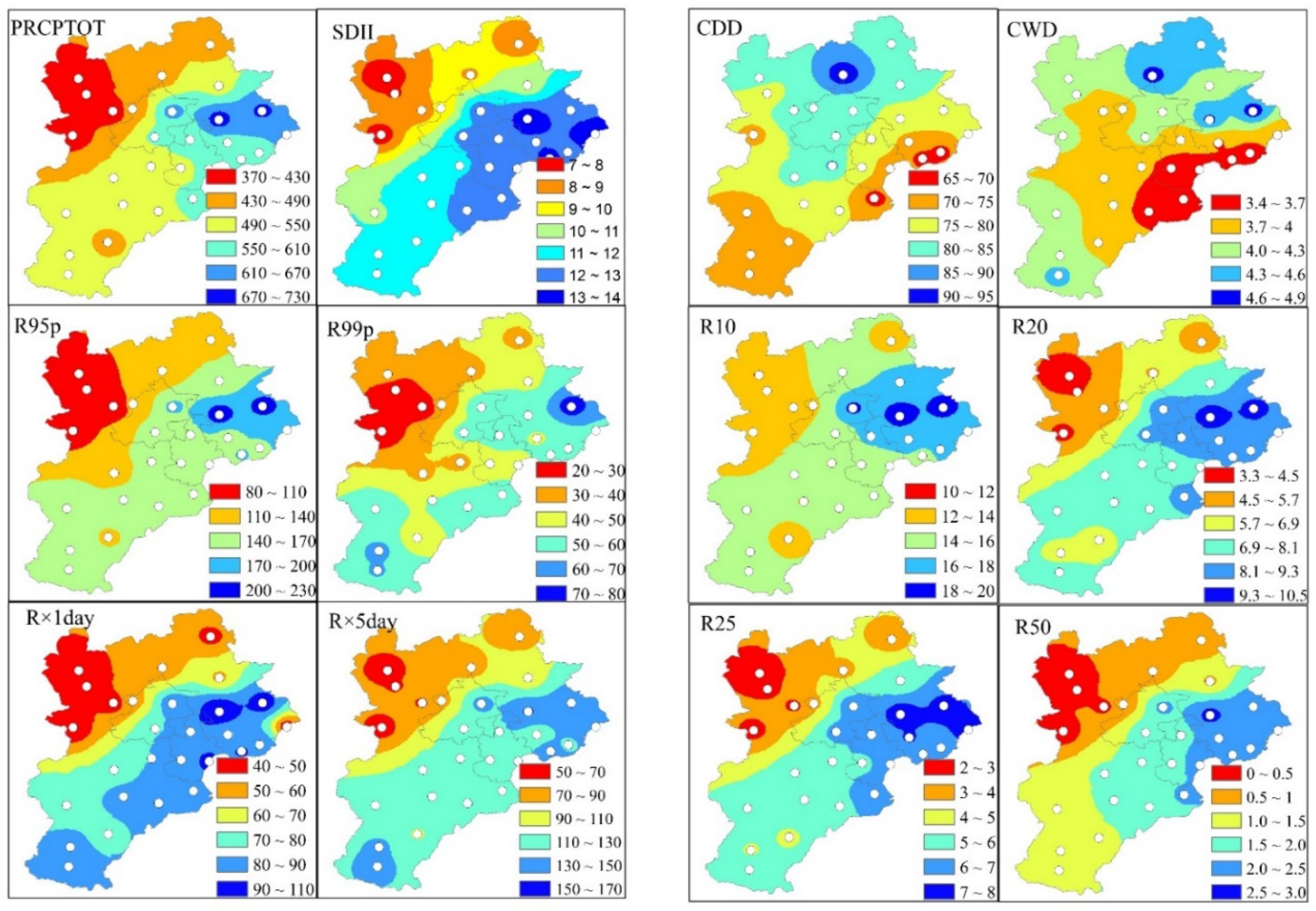
The spatial distribution of precipitation extremes over the BTH region from 1958 to 2017 was shown in Figure 2. In general, the spatial distributions of precipitation extremes apart from consecutive dry days (CDD) and consecutive wet days (CWD) were similar to that of annual precipitation in BTH, with the highest values in the northeast and the lowest in the northwest (Figure 1b). In terms of PRCPTOT, the highest value (709.8 mm in Zunhua station (No. 13)) was observed in the northeast while the lowest value (375.1 mm in Zhangbei station (No. 1)) was found in the northwest of BTH. Similarly, the SDII varied from 7.2 mm/day (Zhangbei station (No.1)) to 13.8 mm/day (Zunhua station (No. 13)), with the high values (12–14 mm/day) occurring on the east coast around the Bohai Bay. Spatial patterns in R95p and R99p were similar, with the largest being observed in the northeast and the lowest in the northwest. The indices in R × 1day and R × 5day increased from the northwest to the southeast, with the highest value of 105.8 mm and 153 mm in Zhangbei station (No. 1). However, the low value (43.5 mm) in R × 1day also occurred in Qinhuangdao station, which was only about half value of the nearest stations (80–90 mm). On the other hand, the value of R × 5day in Qinhuangdao (143 mm) match with its surroundings (130–150 mm). The mean values of CDD were greater in the northwest of BTH than those in the southeast, with the highest value of 94.2 days in Fengning station (No. 6) and the lowest value of 67.6 days in Caofeidian station (No. 21). Only about 10.7% of locations (Fengning (No. 6), Laoting (No. 22), and Huanghua (No. 27), all around the Bobai Bay) in CDD index were less than 70 days, while about 42.9% of stations (covering Beijing city and the northern part of Hebei province) were larger than 80 days. The spatial pattern of CWD was most unique, with the high value in the north and south and the low value in the middle of the region. Specially, the lowest value of CWD occurred in the eastern coast around the Bohai Bay with the value ranging from 3.4 to 3.7 days. In terms of R10, R20, R25, and R50, the spatial patterns were similar, with a decrease from the east to the west. Overall, the spatial patterns of precipitation extremes found in this study agree well with the findings from Mei et al. [33]. The landforms in the northern and western parts of BTH are of a mountainous nature, which act as orographic barriers for the advancing air masses and limit precipitation distribution [69].

3.2. Temporal Variations Extreme Precipitation Events

3.2.1. Annual Scale Trends in Extreme Precipitation Indices

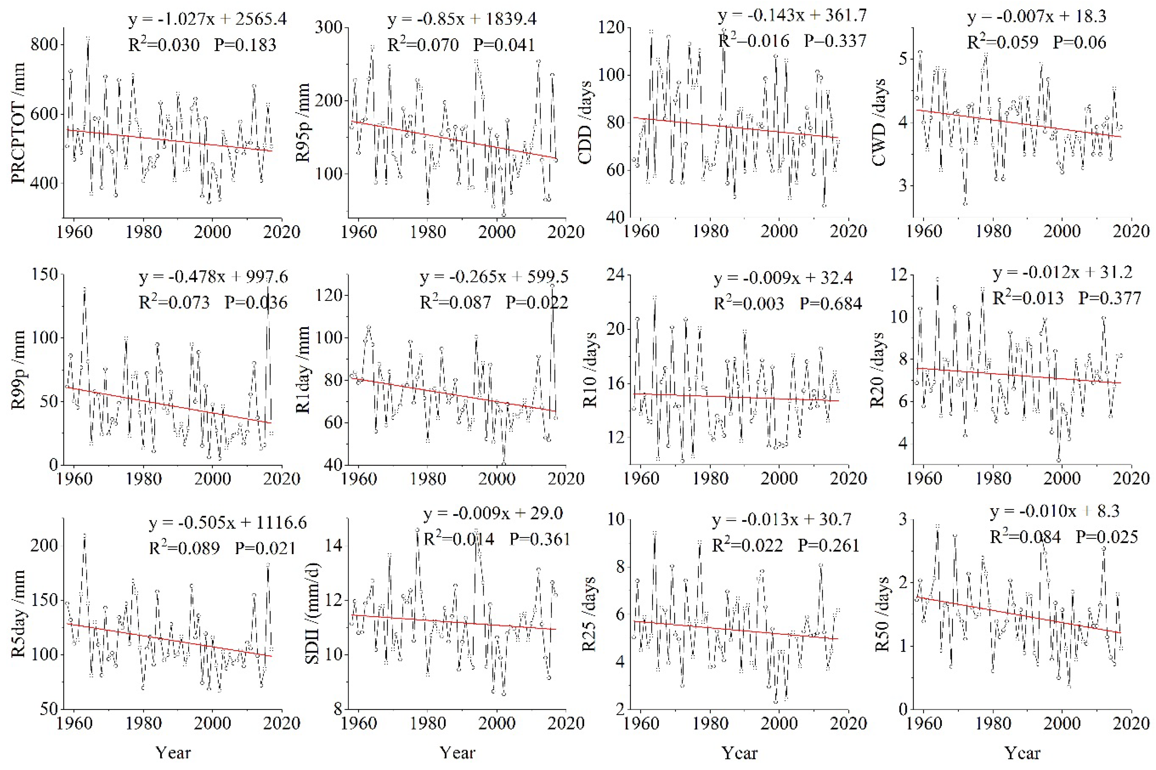
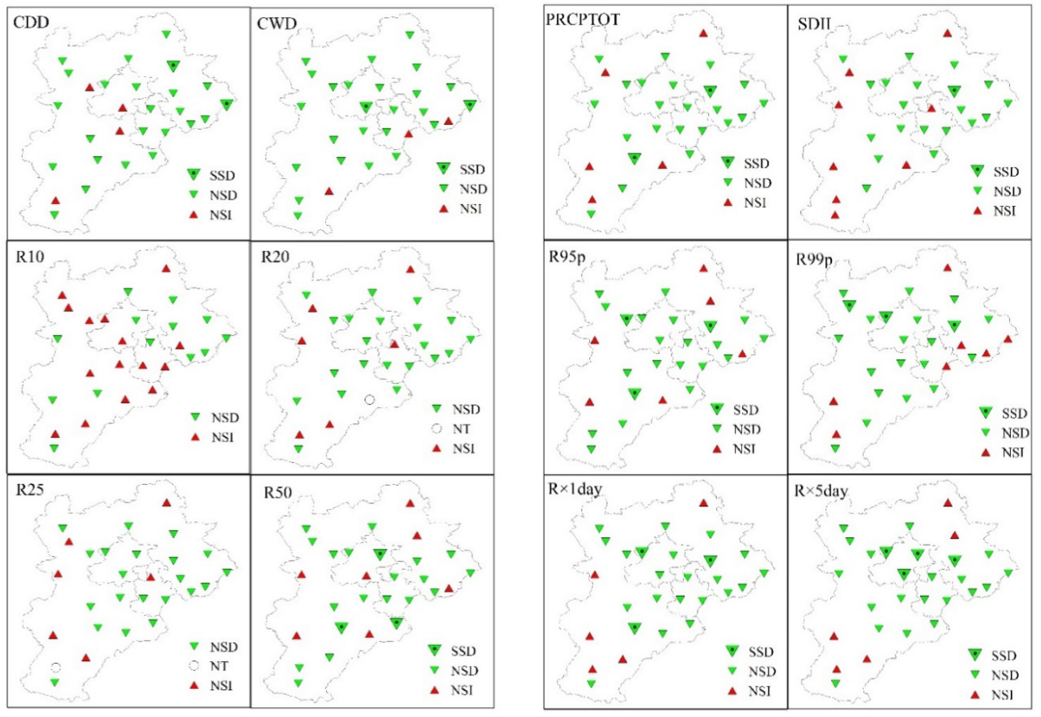
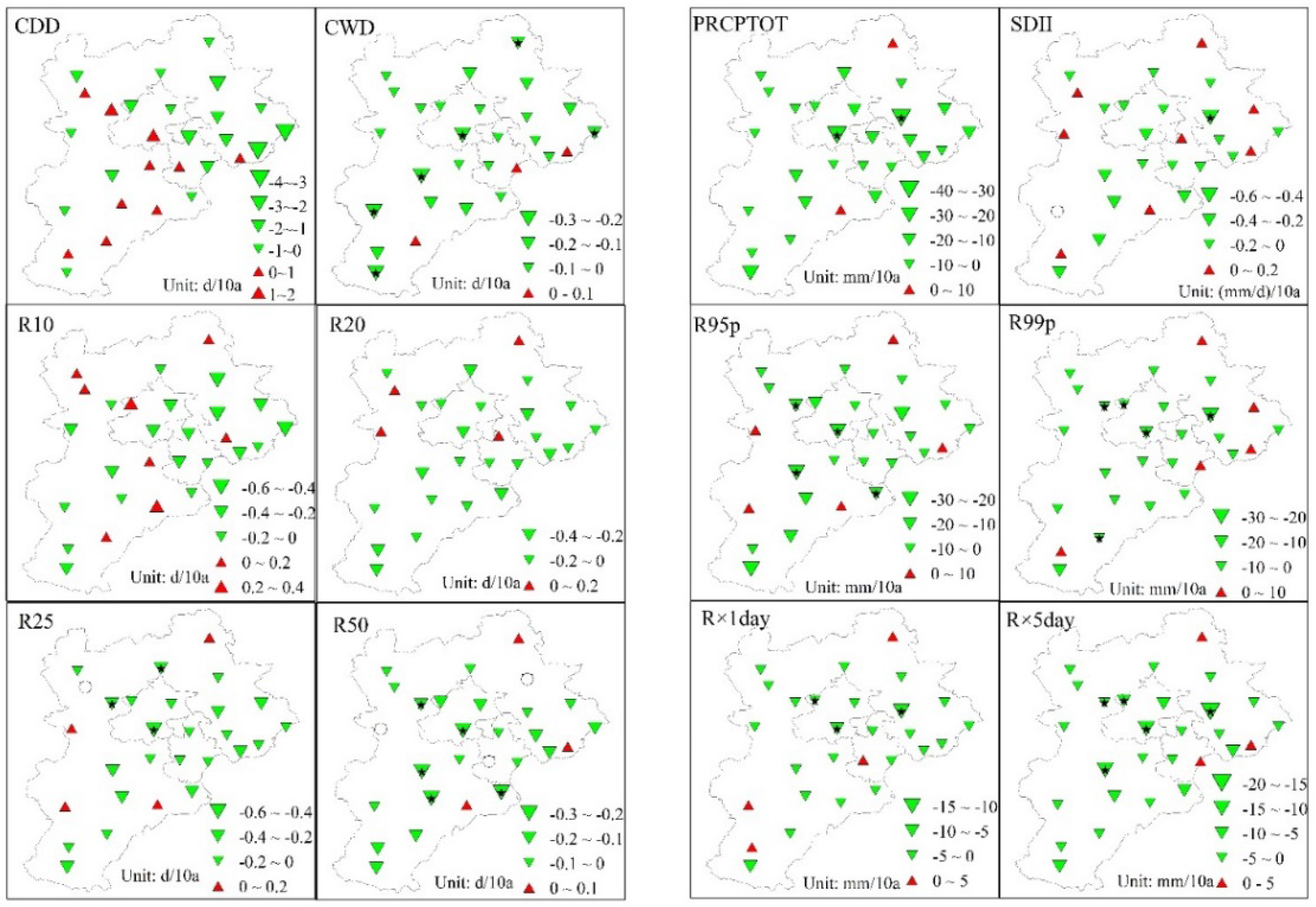
To analyze overall changes in extreme precipitation of BTH in 1958–2017, Figure 3 shows the average annual time series of BTH for all indices, while Table 3 shows the number of individual stations detected with positive or negative trends for the indices analyzed in the study. The spatial patterns of these results are shown in Figure 4 and Figure 5 based on the Mann-Kendall and linear regression method, respectively. Overall, in these indices, negative trends dominate over positive trends, which mean that extreme precipitation over BTH shows more decreasing than increasing trends in the study period.
Over 1958–2017, all the indices showed a decreasing trend based on the linear regression method, while only five indices (R50, R95p, R99p, R × 1day, and R × 5day) showed a statistically significant decreasing trend (p ≤ 0.05) during this period, at a rate of 0.1 day/decade, 8.5 mm/decade, 4.78 mm/decade, 2.65 mm/decade, and 5.05 mm/decade, respectively. As for the average time series of PRCPTOT, it exhibited a non-significant (p = 0.183) decreasing trend at a rate of 10.27 mm/decade, whereas the average SDII time series of BTH had decreased by 0.09 mm/d per decade. The CDD, ranging from 45 days to 119 days with a mean value of 77.8 days, had a decreasing trend at a rate of 1.43 days/decade from 1958 to 2017. The decreasing trend (p = 0.06) for CWD was more significant than that for CDD (p = 0.337) although the decreasing rate of CWD is relatively lower (0.07 day/decade). The regionally averaged occurrence of heavy precipitation days (R10) and heavier precipitation days (R20 and R25) have decreasing trends, nonetheless, they were not statistically significant. The decreasing rates in R10, R20, and R25 were 0.09, 0.12, and 0.13 day/decade, respectively. Similar trends can be also concluded from the Mann-Kendall trend test, as shown in Table 3. All the indices except R10 had a decreasing trend, but also only five indices (i.e., R50, R95p, R99p, R × 1day, and R × 5day) showed a statistically significant decreasing at the 0.05 level.
Overall, the preponderance of evidence indicated that the decline trends in indices were more frequent than the increasing ones although considerably few decreasing trends exceeding 95% confidence level during 1958–2017. However, there are slight discrepancies in trends between the Mann-Kendall test and the linear regression. Compared with Mann-Kendall test, the greater number of stations (34 versus 23) with significantly decreasing trends are found based on linear regression. Additionally, based on the Mann-Kendall test, about 53.6% (46.4%) of the stations showed upward (downward) trends for R10, while none of these trends are statistically significant. On the contrary, most of stations (71.4%) for R10 showed negative trends based on the result of linear regression method. For the other indices, the similar trends can be found based on the two methods. Generally, although most of locations exhibited downward trends for the precipitation extremes, less than 25% of them showed significant decreasing trends in the BTH region during 1958–2017.

3.2.2. Monthly and Seasonal Changes in Precipitation Extremes

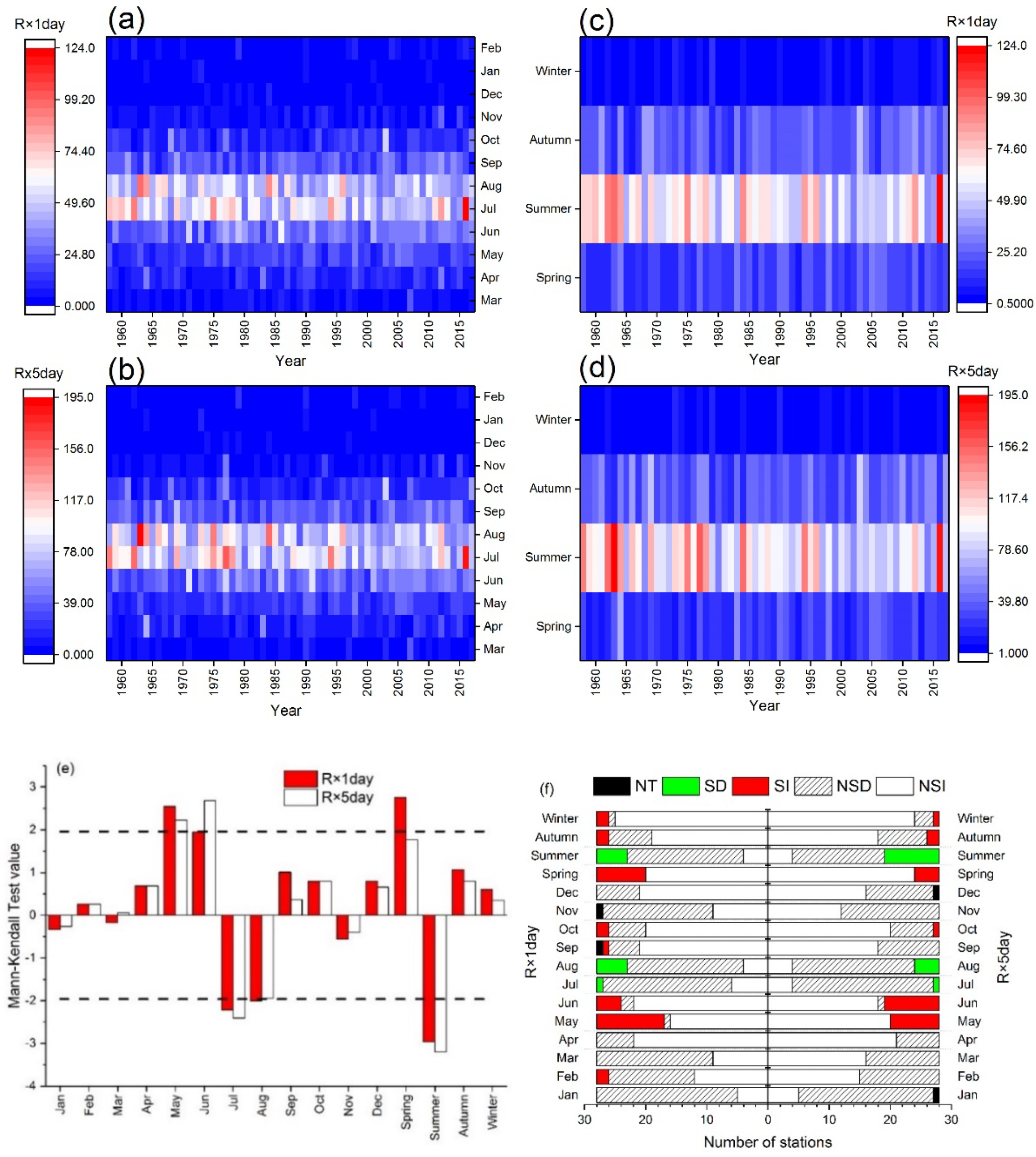
In this study, R × 1day and R × 5day were used to analyze the monthly and seasonal changes in precipitation extremes, as shown in Figure 6. It was found that the monthly mean values in R × 1day and R × 5day during the period of 1958–2017 varied from 1.6 to 56.1 mm, and 2.4 to 88.7 mm, respectively. The wettest season in BTH is summer (June-July-August) due to effects of eastern Asian Monsoon climate, of which the precipitation amount accounts for about 70% of annual totals [67]. Obviously, almost all of the highest values in R×1day and R×5day occurred in summer (both about 98.3% of totals), especially in July (37 and 36, respectively) and August (19 and 22, respectively). And the lowest values frequently occurred in winter (December-January-February). On average, the highest values of R × 1day and R × 5day occurred in July (28.6~123.8 mm and 41~182.3 mm, respectively) and the lowest in January (0.02~9.7 mm and 0.1~14.1 mm). The trends of monthly and seasonal time series were also detected by the Mann-Kendall test, as shown in Figure 6e. In terms of R × 1day, a significant increasing trend was found in May while a significant decreasing trend occurred in July and August, which may result the trend of significant upward in spring and significant downward in summer. Other monthly and seasonal series also had increasing or decreasing trends but are not significant at the level of 0.05. Similarly, a significant increasing (decreasing) trend in May (July and summer) was also found in R × 5day. However, a significant upward trend for R × 5day was also detected in June. Overall, the decreasing trend in summer (especially in July and August) may be the cause the decreasing trend in annual series. Furthermore, the statistical results of trends for all the stations are shown in Figure 6f. An increasing trend was dominant in spring (100% of locations), autumn (75% and 71.4%) and winter (96.4% and 89.3%) for R × 1day and R × 5day, respectively, while about 85.7% of locations showed a downward trend in summer for both indices. Certainly, the number of significantly increasing or decreasing trends (SI or SD) was less than that of non-significantly increasing or decreasing trends (NSI or NSD) for all the seasons. Analogously, the monthly series can also be classified by two groups except February and March. One was dominated by increasing trends, including April, May, June, September, October, and December, and the other was leaded by decreasing trends, including January, July, August, and November. In February, the stations with increasing or decreasing trends both accounted for about half of the totals in R × 1day (50%) and R × 5day (53.6% and 46.4%). Interestingly, in March, more stations showed decline trends in R × 1day, whereas the opposite results were found in R × 5day. In conclusion, the decline trends in annual series may be caused by significant decreasing trends in summer, especially in July and August. Although significant increasing trends were also found in several months or seasons, their effects on the trends in annual series were less than that in summer, because most of values in the annual series occurred in summer.

3.2.3. Decadal Variability in Precipitation Extremes

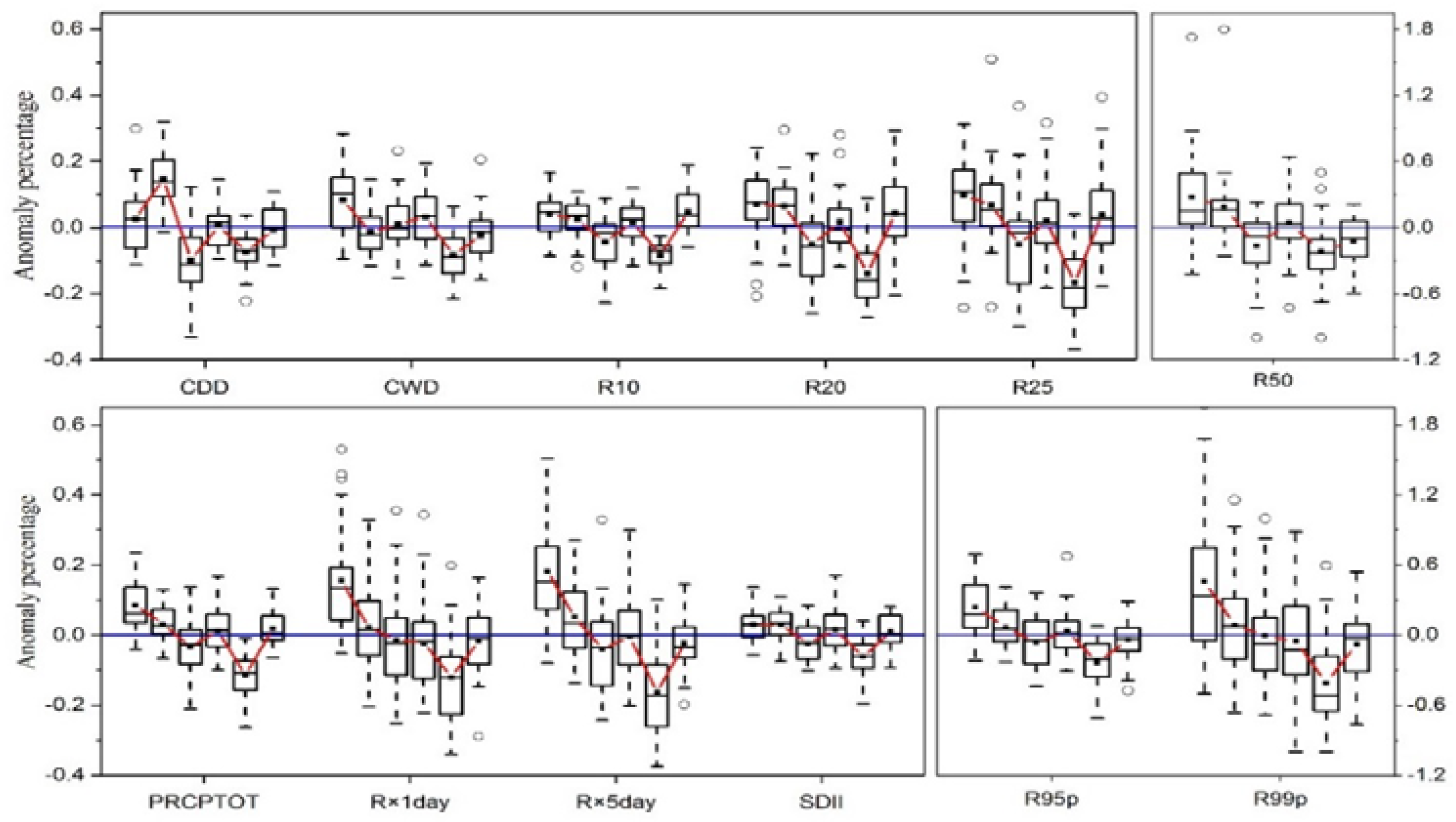
We divided the period 1958–2017 into the following six sub-periods: 1958–1967 (T1), 1968–1977 (T2), 1978–1987 (T3), 1988–1997 (T4), 1998–2007 (T5), and 2008–2017 (T6). Anomaly percentages of decadal mean precipitation extremes for all the stations were also calculated to analyze their variations, as shown in Figure 7. The detailed information of precipitation extremes in each sub-period can be found in Table S1. It was found that all the maximum values of decadal mean indices for sub-period occurred in T1, except for CDD (T2) and R10 (T6), while all the minimum values except CDD (T3) occurred in T5. The decadal changes in CDD suggested that the BTH appeared more dryness in T2 because of the higher consequence dry days, and the discrepancies ranged from 9.5 to 19.3 days (about 12.2–24.8% of mean value in CDD during 1958–2017) compared with the other sub-periods. The results from the other indices suggested that the extreme precipitation events or flood events may be more acute in T1 over BTH, whereas the relatively less probability or weights of extreme precipitation events occurred in T5. Figure 7 also showed that there were greater variations in R50, R95p, and R99p compared with other indices, which mean the higher spatial variations. Additionally, it was worth noting that all the indices except CDD experienced clear fluctuations among these sub-periods with a complex trend of decreasing (from T1 to T3)—increasing (from T3 to T4)—decreasing (from T4 to T5)—increasing (from T5 to T6).
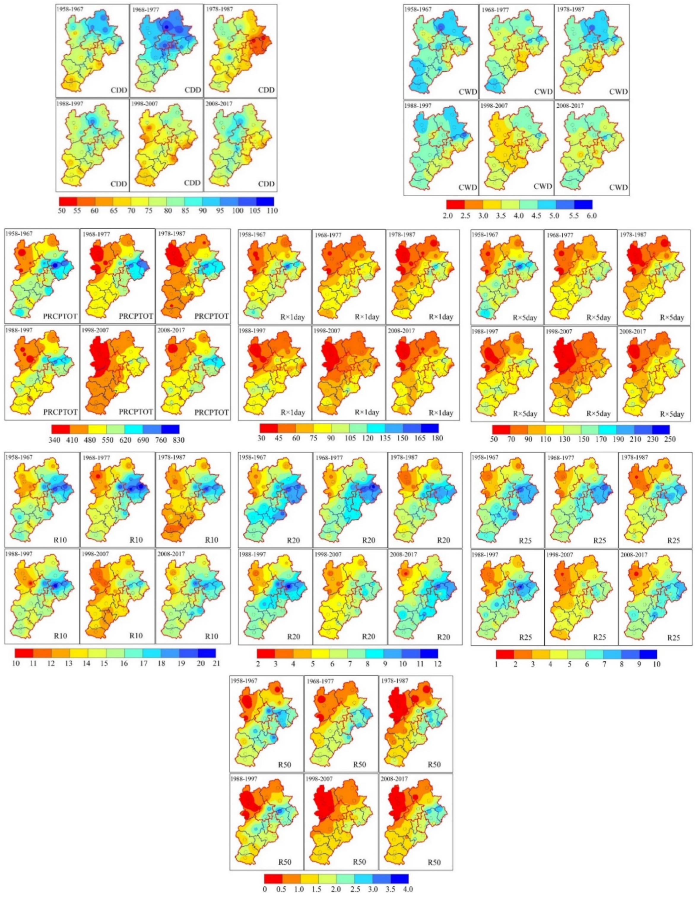
In order to further analyze inter-decadal changes for precipitation extremes, Figure 8 demonstrated decadal changes for all the extreme precipitation indices. In general, the spatial patterns for all the indices in the six sub-periods were similar with slight variations. That is, the spatial distributions in each sub-period had no any significant change, which agreed well with that in the entire period of 1958–2017. As mentioned previously, the decadal changes in CDD were different from the other indices. About 42.9% of stations in the CDD in T2 was larger than 90 days, covering about 54.5% of BTH, while only one station in T3 was larger than 90 days. In T3 sub-period, the lowest value of the CDD located in the east of BTH, less than 60 days. In terms of CWD, in T2, T5 and T6 sub-periods, the lower values occurred in the middle of BTH, while the higher values located in the southern and northern areas of Hebei province. However, in T1 and T4, the lowest value of CWD located in the eastern part of the BTH region. In T1 sub-period, about 35.7% of locations in PRCPTOT was larger than 620 mm, mainly located in the eastern BTH and the south of Hebei province. However, none of them was higher than 600 mm in T5, and PRCPTOT for all the stations except Zunhua (No. 13) and Qinglong (No. 14) stations (located in the eastern BTH) was less than 550 mm. The similar decadal variations were found in R × 1day and R × 5day. The decadal averages of R × 1day and R × 5day had a same pattern of “high value in the southeast and low value in the northwest” for different sub-periods. The similar decadal variations and spatial patterns can be obtained for the indices of precipitation days (e.g., R10, R20, R25, and R50). In terms of R95p and R99p, the spatial patterns are different, with the lowest value occurring in the middle of the BTH region in T5 and in the western mountain areas during the other sub-periods. For the index of SDII, there was no difference among the six sub-periods, with the same spatial patterns of “high value in the southeast, and low value in the northwest”.

3.2.4. Periodicity Analysis of Extreme Precipitation Indices

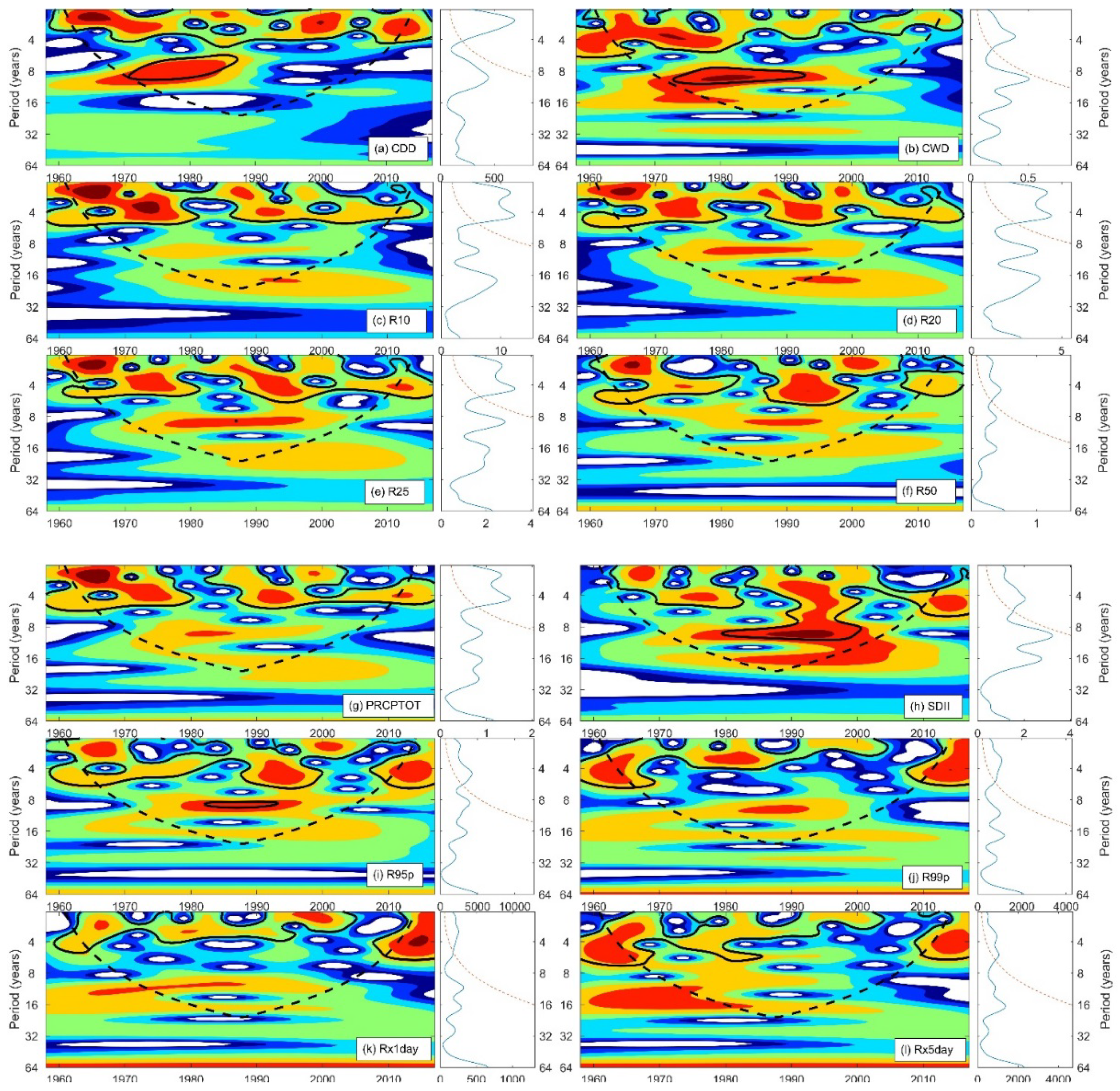
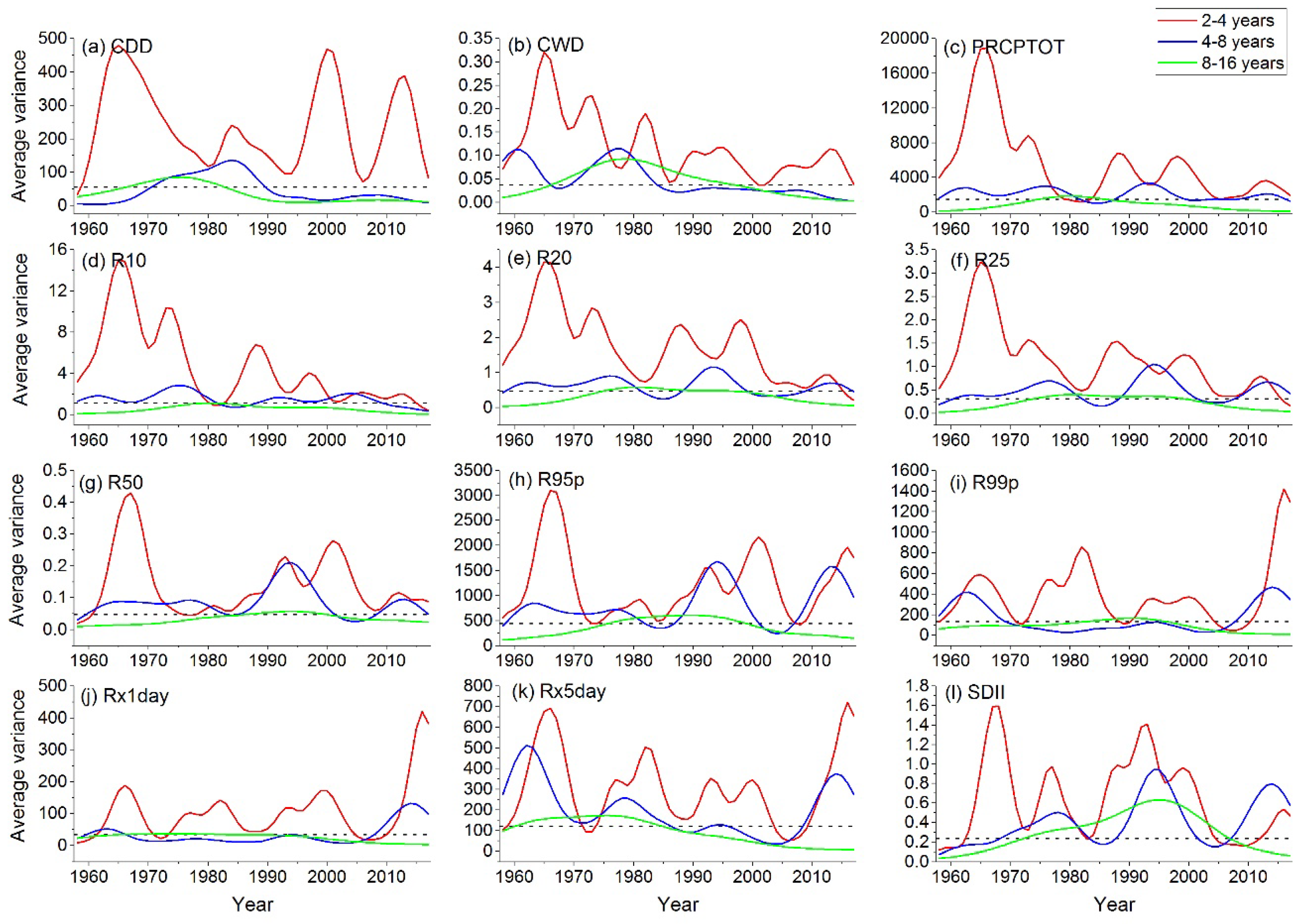
The wavelet power spectra of the regional average series of precipitation extremes over the BTH region were shown in Figure 9. We can observe significant periodic oscillations in all indices. For all the indices, the significant two- to five-year periods at the 5% level were predominant during 1958–2017. Furthermore, the CDD wavelet power spectrum showed 6–10-year modulations of variation, which occurred in the 1970s to the mid-1980s. Similarly, the significant inter-decadal (approximately 8–11 years) oscillations were active from the 1970s to the 1980s. For SDII, the power was broadly distributed, with a period of 2–11 years from the 1990s to 2000, and with a period of 8–11 years in the 1980s. Additionally, continuous wavelet spectrum for R95p also showed the significant wavelet power at 8–10 years during 1982–1993. The global wavelet power spectrum (GWPS) is an equal-weighted average of all the local wavelet power spectra for each scale, which shows dominant scales with no temporal transformation (Figure 9). Regional averaged GWPS shows a statistically significant low-frequency oscillation with a period of 2–9 years in CDD, a period of 2–12 years in CWD, a period of 2–8 years in R10, R20, R25, and RPCPTOT, a period of 2–10 years in SDII, a period of 2–14 years in R95p, a period of 2–15 years in R50 and R99p, and a period of 2–16 years in R × 1day and R × 5day. According to the local wavelet spectra (Figure 9), inter-annual (2–4 years and 4–8 years) and inter-decadal (8–16 years) time scales are significantly above the red noise background spectra over certain time periods. Therefore, these three scale bands (2–4 years, 4–8 years, and 8–16 years) were selected to compute the scale-averaged wavelet power (SAWP), as shown in Figure 10. The results showed that significant inter-annual (2–4 years) oscillations for all the indices almost occurred during the entire period of 1958–2017. In terms of CDD, significant inter-annual (4–8 years) oscillations occurred in the 1970s and 1980s, while inter-decadal oscillations were active from 1966 to 1982. For the index of CWD, significant inter-annual (4–8 years) fluctuations occurred in the periods of 1958–1984 and inter-decadal oscillations were active from 1966 to 1996. PRCPTOT showed an obvious inter-annual (4–8 years) oscillations during the entire period and inter-decadal oscillations during 1974–1986. For R10, R20, R25 and R50, the significant inter-annual oscillations were almost active in the entire period, but inter-decadal oscillations occurred in 1980s for R20 and R25, and in 1990s for R50. Both R95p and R99p showed significant inter-annual fluctuations in 1960s–1990s, and obvious inter-decadal oscillations in 1980s–1990s. Inter-annual oscillations for R × 1day and R × 5day were active from 2009–2017 and inter-decadal oscillations occurred in 1970s. Moreover, the extra inter-annual oscillations for R × 5day were also significant during 1958–1986. SDII showed relatively longer inter-decadal oscillations during 1973–2007.

3.3. Relationship Between Precipitation Extremes and Annual Total Precipitation

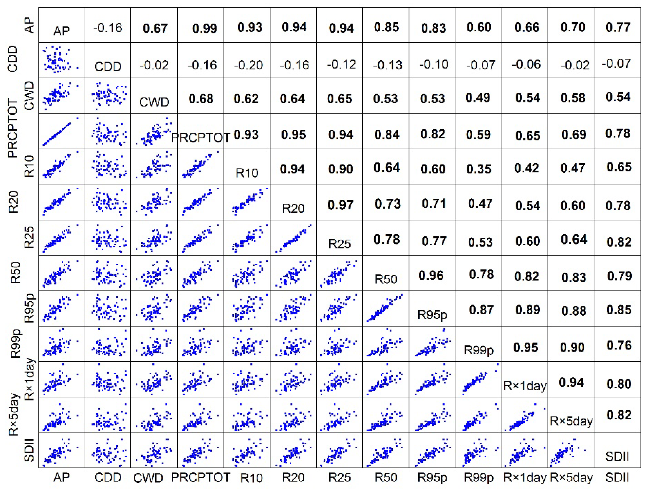
Previous studies have indicated that the annual total precipitation correlates well with extreme precipitation [33,70,71,72]. In this study, we estimate the Spearman’s rank correlations between the extreme precipitation indices and annual total precipitation, as shown in Figure 11. All the indices except CDD showed significantly positive correlations at a level of α = 0.05. The correlation coefficients between extreme indices and total precipitation exceeded 0.6, except for CDD, which implied that these precipitation extremes had significant correlations with annual precipitation, especially the PRCPTOT, R10, R20, and R25 (correlation coefficient >0.90). Therefore, the decrease in precipitation extremes over BTH reflect the decrease in annual total precipitation to some extent, which match with the finding of previous studies [69]. In reverse, the decline in precipitation extremes mainly caused by the descend in annual total precipitation. Figure 11 also illustrates the correlation coefficients among the extreme precipitation indices. Except for CDD, all the indices have a significant correlation with most of the coefficients higher than 0.5 (p < 0.01). The weak negative correlations between CDD and the other extreme precipitation indices were also found in Figure 11.

3.4. Possible Linkage to Large-Scale Atmospheric Circulation Patterns

As discussed in previous parts, the large-scale circulation patterns have affected the climate in China. As large-scale ocean-atmospheric phenomena may influence precipitation extremes in one year and the next year [41], the effects of one-year and 0-year ahead ENSO, NAO, PDO, and IOD on the annual precipitation extremes were investigated in this study to fully identify their relationships. The indices of climate variability in previous year (NINO3.4-1, NAO-1, IOD-1, and PDO-1) (i.e., time series of climate indices: 1957–2016) and this year (NINO3.4-0, NAO-0, IOD-0, and PDO-0) (i.e., time series of climate indices: 1958–2017) are used to estimate the Spearman’s correlations with precipitation extremes in this year, as illustrated in Table 4. We found that most of extreme precipitation indices in the BTH region were significantly influenced by ENSO with one-year ahead (NINO3.4-1). The p-value for the correlations between NINO3.4-1 and CDD, PRCPTOT, R10, R20, and R25 is less than 0.01. However, almost of all the regional averaged indices were not significantly influenced by the other climate indices, especially for NAO-1, POD-1, and POD-0 with none of extreme indices being significant correlation at 5% and 10% significant levels. Interestingly, almost all the extreme indices have a converse correlation with the climate indices in previous and present year. For example, CDD is positively correlated with NAO-0 but it has a negative correlation with NAO-1, as shown in Table 4.
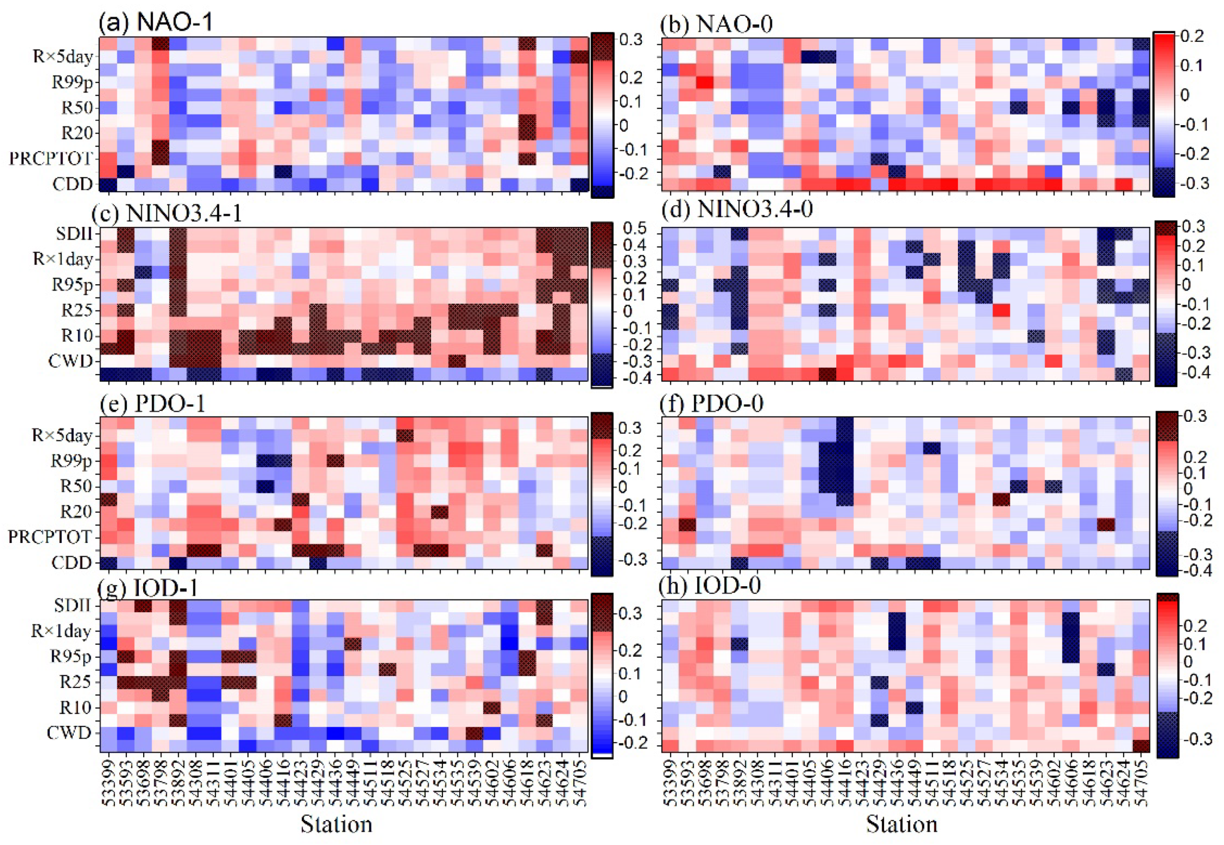
Additionally, for each station, the correlation coefficients are illustrated in Figure 12. It can be seen that the areas with positive correlations between precipitation extremes and atmospheric circulation indices with one-year ahead were larger than those with 0-year ahead. For instance, about 54.2% of extreme indices is positively correlated with NAO-1, while about 77.7% of them is negatively correlated with NAO-0. Similar conclusions can be obtained from other climate indices, with about 84.8%, 50.9%, and 72.3% of extreme indices being positively correlated with NINO3.4-1, PDO-1 and IOD-1, respectively. Moreover, about 80.1%, 66.7%, and 61.9% of extreme indices are negatively correlated with NINO3.4-0, PDO-0, and IOD-0, respectively. Overall, from the view of the statistical analysis, extreme precipitation events in the annual scale over the BTH region may be significantly influenced by ENSO (NINO3.4) and relatively weaker influenced by the other atmospheric circulation indices.
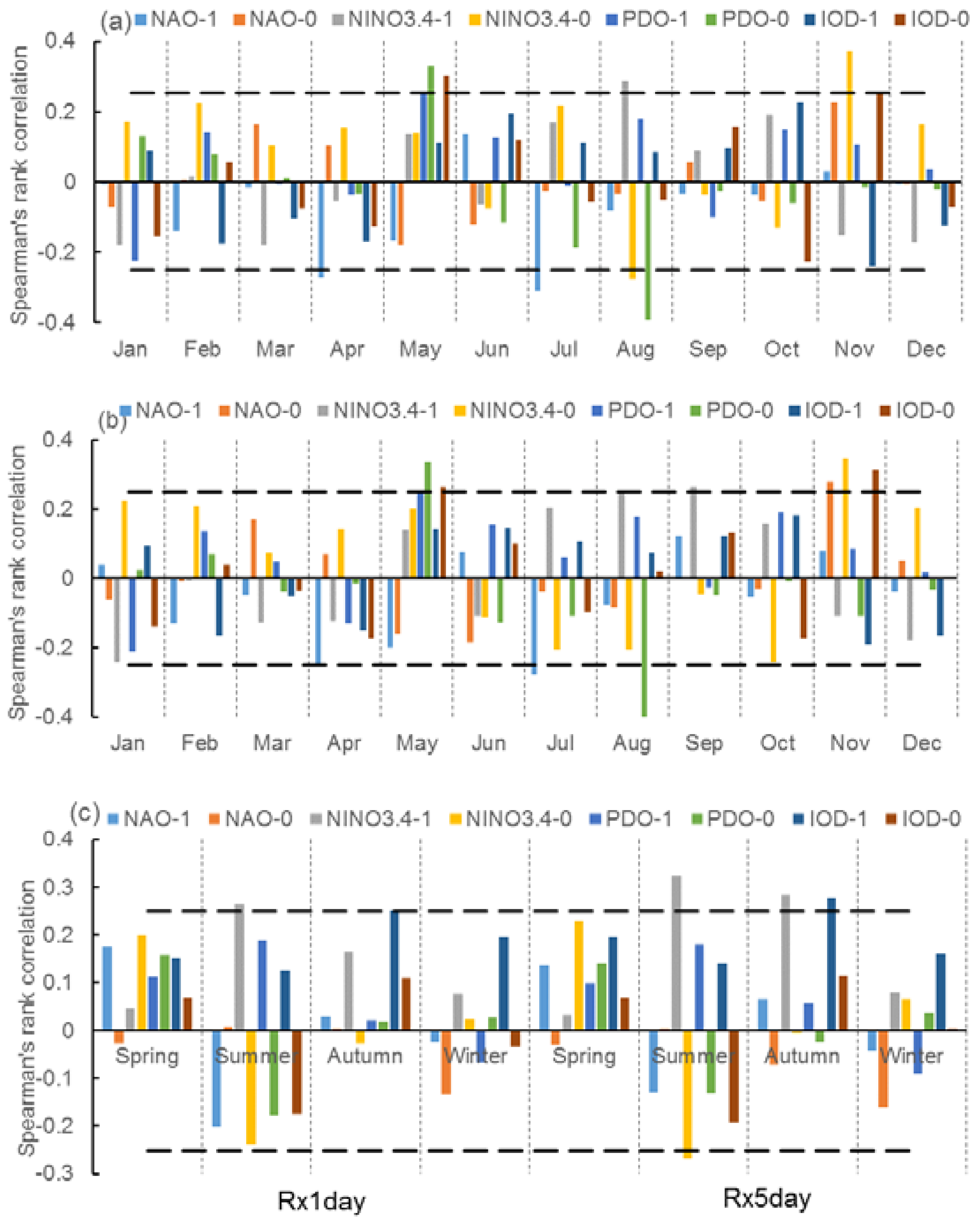
In this study, monthly and seasonal R × 1day and R × 5day were also used to analyze their relationships associated with the climate indices, as shown in Figure 13. In terms of monthly R × 1day, Figure 13a showed that significant correlation occurred in April (NAO-1), May (PDO-1, PDO-0), July (NAO-1), August (NINO3.4-1, NINO3.4-0, PDO-0), and November (NINO3.4-0 and IOD-0) at a significance level of α = 0.05. A similar conclusion can be seen for monthly R × 5day in above five months (Figure 13b). Additionally, R × 5day in September showed a significantly correlated with NINO3.4 in previous year. In terms of seasonal series, extreme precipitation in summer and autumn are significantly influenced by large-scale atmospheric circulation. For example, R × 1day and R × 5day in summer are significantly correlated with the NINO3.4-1, and R×5day in summer is also significantly influenced by NINO3.4-0. R × 1day and R × 5day in autumn are significantly correlated with the IOD-1, and R×5day in summer is also significantly influenced by NINO3.4-1.
To fully understand their teleconnections, the periodic structure of precipitation extremes and large-scale atmospheric circulation indices are considered and estimated in this study. Based on the length of the original series, we have chosen a suitable scale to construct the periodic components of the original series in the wavelet transforms. As Figure 11 showed, precipitation extremes have the significant oscillation with a scale of 2-16 years during a certain period. Therefore, we selected 2, 4, 8, and 16 year scales to develop the periodic components of the precipitation extremes and climate indices. In this study, we applied the CWT approach to decompose the original series into four identical resolutions, i.e., two-year periodicity (C1), four-year periodicity (C2), eight-year periodicity (C3), and 16-year periodicity (C4). The Spearman’s correlations between the decomposed series (C1, C2, C3, and C4) of precipitation extremes and that of the large-scale atmospheric circulation indices were calculated, as shown in Table 5. We found that almost half of precipitation extremes were significantly correlated with NINO3.4-0 at different periodic components, but the significantly correlations between precipitation extremes and NINO3.4-1 mainly occurred in C1 and C4. The visibly opposite correlations between precipitation extremes and NINO3.4 with one-year ahead and 0-year ahead were shown for C1, whereas the same correlations were found for C4. All the extreme indices except for R99p and R×1day showed a significantly positive correlation with the low-frequency component (C4) of NAO, and nine of extreme indices also showed a significantly positive correlation with NAO-1 for C2. Most of precipitation indices were significantly correlated with PDO for the low-frequency components (C3 and C4), accounting for 87.5% (PDO-0) and 66.7% (PDO-1). Moreover, almost all the indices for C1 showed significantly positive correlation with PDO-1 except for CDD and R50. In terms of IOD, eight of extreme precipitation indices at C4 were significantly correlated with IOD-0 and IOD-1, and almost all of them showed a significantly positive correlation with IOD-1 for C2. Overall, the influences of climate indices on regional precipitation extremes were composed by different periodic components, with the higher correlations mainly occurring at a low-frequency component (e.g., C4). However, the discrepancies of correlations between precipitation extremes and climate indices with 0-year and one-year ahead mainly occurred at a high-frequency component (e.g., C1).

4. Discussion

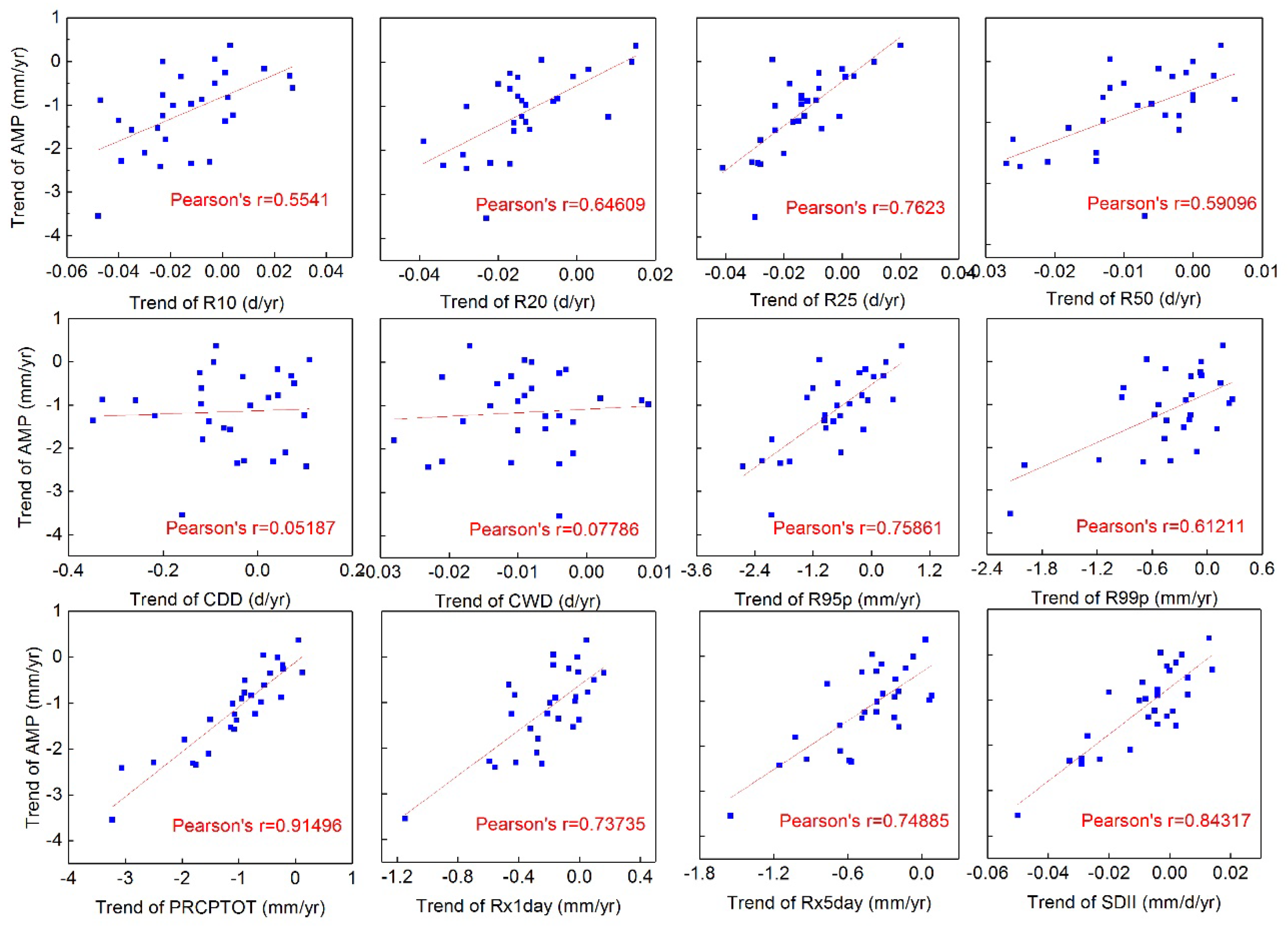
Previous studies have reported that extreme precipitation has changed over the past few decades, but there are apparent discrepancies in regarding these changes over different regions in China, including BTH or North China [73]. Overall, the temporal trends in our work are similar to previous studies in reporting decreasing trends in precipitation extremes over the past few decades in BTH [33,36,40] and the Circum-Bohai-Sea region in the north of China [63,74]. Certainly, there are some discrepancies between our work and previous studies. For instance, Mei et al. [33] found that the significantly decreasing trends were only shown in R × 1day and R × 5day during 1960–2013. But we found that more indices (e.g., R50, R95p, and R99p) exhibited significant decreasing trends in BTH during 1958–2017 (Figure 3 and Table 3). In terms of spatial patterns of precipitation extremes, our results are also consistent with the previous studies in BTH or neighboring regions. Overall, for most of precipitation extremes except for CDD and CWD, the highest values located in the eastern BTH region, while the lowest values occurred in the western part (Figure 2), which was mainly influenced by the terrain (Figure 1a) with the high values in the northwest and the low in the southeast of BTH. Spatial patterns of precipitation extremes are similar to that of annual total precipitation (Figure 1b and [69]) with high correlations (Figure 11), which was consistent with previous studies [6,33]. The correlations between the trend magnitudes of annual total precipitation and precipitation extremes for all the stations were also estimated, as shown in Figure 14. All the extreme precipitation indices were positively correlated with annual total precipitation, which is also different from that found in Mei et al. [33]. In Mei’s work, they found the annual trend magnitudes of CDD and CWD were negatively correlated with that of annual total precipitation (ATP), with the correlations being significant for CDD. However, in our study, all the precipitation extremes are statistically significant at the 0.05 level except for CDD and CWD. The discrepancies may be caused by the data with different time periods used in the two studies. Furthermore, we also analyzed variations of the monthly, seasonal and decadal precipitation extremes, which has been reported in the other regions [64,75,76] but not in the study area [33,36,40]. As all known, North China has a monsoon climate with salient four seasons and about 60–80% of total precipitation amount in summer. Thus, it is helpful to understand the annual variations by the analysis of monthly or seasonal changes in precipitation extremes. We found that the decreasing trends in annual precipitation extremes were mainly caused by the descend in summer, especially in July and August (Figure 6). Although the significantly increasing trend can be found in many months or seasons (Figure 6), their increases have not remedied the descends of annual R × 1day and R × 5day over BTH.
As previous mentioned, changes in precipitation extremes are related to the large-scale circulation change [41,42,77,78,79]. The periodicity characteristics of precipitation extremes will be helpful to understand their associations or linkages with climate indices, which has been investigated in the other regions in previous studies [40,60,61,62,63,64,65]. Our results showed that the significant two- to five-year periods at the 5% level were predominant for all the indices during the entire period, which are roughly consistent with the previous work of Wang et al. [63]. As pointed by Moron et al. [77], there are appropriate evidences that both the quasi-biennial (2–3 years) and quasi-quadrennial (4–6 years) peaks of climate variables are related to ENSO. That is, the inter-annual (2–5 years) oscillation in extreme precipitation over BTH may be influenced by ENSO, which was also verified based by the correlation analysis (Table 4 and Table 5). Moreover, quasi-decadal oscillations of precipitation extremes were also detected. Furthermore, to better understand their relationships between precipitation extremes and climate anomalies, the quantitative analyses should be conducted. However, the correlations between precipitation extremes and climate indices over BTH or north China has not been examined or fully explained in the previous studies. Thus, we computed the correlations between the precipitation extremes and large-scale climate anomalies to reveal their relationships. Our results showed that most of extreme precipitation indices in the BTH region were significantly influenced by ENSO with one-year ahead (Table 4 and Figure 10), which are consistent with the finding in Xiao et al. [41] and Gao et al. [79]. Besides, we also found that almost all the extreme indices exist a converse correlation with the climate indices in one-year ahead and 0-year ahead. That is, the relationships of annual extreme precipitation indices with the climate indices are different when the climate indices are at different stages [41]. Moreover, the precipitation extremes in different months were influenced by different climate indices or more than one index (Figure 11). To some extent, our results also showed that precipitation extremes at any scale are influenced by many climate indices together. As previous studies mentioned, the climate of eastern China is dominated by the East Asian Monsoon, which is significantly influenced by ENSO [80,81]. Meanwhile, the East Asian Monsoon is also influenced by NAO, PDO, and IOD, and then affect the regional patterns of precipitation or precipitation extremes. Our findings also provide an illustration for this conclusion.
Overall, in this study, the spatio-temporal variation and characteristics of precipitation extremes in the BTH region were studied using various methods, and useful information was obtained, which is potentially is useful for natural disaster prevention and mitigation. In this study, we use the simple linear regression and Mann-Kendall test to detect the trends of precipitation extremes. Linear regression method, one of parametric tests, can be capable of quantifying the change in the data, which assumes the time series and the errors following a normal distribution. A normality test of regional precipitation extremes is detected using one-sample Kolmogorov-Smirnov test method, which clearly indicates that all the data can be regarded as normally distributed. Mann-Kendall trend test, one of the widely used non-parametric tests, being a function of the ranks of the observations rather than their actual values, is not affected by the actual distribution of the data and is less sensitive to outliers. Thus, Mann-Kendall test, as well as other non-parametric trend tests, is more suitable for detecting trends in hydrological time series, which are usually skewed and may be contaminated with outliers [82]. A common requirement of both parametric and non-parametric trend tests is that the data be independent [82,83]. In this study, the possible effects of serial correlation have been not considered. However, in the future work, the serial correlation should be detected and eliminated by pre-whitening of the data when these methods are used to detect the trends of hydrologic series. Additionally, the observed data with the sparseness of meteorological gauges (only 28 national-level meteorological stations) may have led to uncertainties and limitation in our results and conclusions, especially in spatial variability [84], which need to be improved in the future work. The higher temporal (e.g., hourly time series) and spatial (e.g., 316 meteorological stations used in Zhao et al. [69]) resolutions would lead to more reliable and specific results. Moreover, the selection of indices of climate extremes is also an important step to assess their variations. A number of indices were suggested, each aimed at depicting a certain aspect of climate extremes. In this study, the 12 precipitation indices were chosen from the indicators recommended by the ETCCDMI. From our findings, several indices showed similar results, especially for these indices belongings to same properties. For instance, the results of spatial patterns and temporal trends in R10, R20, and R25 are almost similar (Table 3, Figure 3, Figure 4 and Figure 5). Thus, in order to quickly and efficiently analyze the variations of precipitation extremes, these similar indicators can be eliminated based on the different demands. One representative index can be chosen for each type of precipitation extremes, such as the percentile-based threshold, and fix-based threshold.
In this study, the possible relationship between precipitation extremes and climate indices is also discussed, including the in-phase and out-of-phase linkages between them. Past studies have revealed that the relationships between precipitation extremes and different teleconnection phases tend to be asymmetrical and generally do not portray linear behavior [85]. Thus, the nonlinear and different influences associated with different phases of these teleconnections have important implications on this issue. Aside from the above two aspects, the multiple-variables jointly relationships between precipitation extremes and climate indices should be also further investigated in the future work. Moreover, the mechanistic understanding of how these climate drivers impact extreme precipitation in BTH through forcing large-scale atmospheric circulation changes need to be further investigated, and the analyses of the physical causes of these variability will form the basis of our future research.

5. Summary and Conclusions

In this work, attempts are made to investigate the long-term changes of precipitation extremes at different scales. The analyses of spatial-temporal variations in precipitation extremes across BTH are conducted with 12 indices based on daily precipitation records from 28 meteorological stations. Moreover, the possible relationships between extreme precipitation events and large-scale atmospheric circulation patterns are also analyzed. Based on the above results and discussion, our mainly findings are summarized as follows:
(1) The spatial distributions of precipitation extremes apart from CDD and CWD were similar to the spatial patterns of annual precipitation in BTH, with the highest in the northeast and the lowest in the northwest. The mean values of CDD were greater in the northwest of BTH than those in the southeast. The spatial pattern of CWD was most unique, with the high value in the north and south and the low value in the middle of the region.
(2) Regionally averaged precipitation extremes were characterized by decreasing trends, of which five indices (R50, R95p, R99p, R × 1day, and R × 5day) exhibited statistically significant decreasing trends at a level of 0.05. From monthly and seasonal scale, almost all of the high values in R × 1day and R × 5day occurred in summer, especially in July and August due to the impacts of East Asian monsoon climate on inter-annual uneven distribution of precipitation. The significant decreasing trends in annual R×1day and R×5day were mainly caused by the significant decreasing trend in summer.
(3) The extreme precipitation events may be more acute in the first decade (T1, 1958–1967) over those areas, whereas the relatively less probability or weights of extreme precipitation events occurred in T5 (1998–2007). All the indices except CDD experienced clear fluctuations among these sub-periods with a complex trend of decreasing (from T1 to T3)—increasing (from T3 to T4)—decreasing (from T4 to T5)—increasing (from T5 to T6).
(4) For all the indices, the significant two- to five-year periods at the 5% level were predominant during the entire period of 1958–2017 based on the wavelet analysis. Specially, there were a statistically significant low-frequency oscillation with a period of 2–9 years in CDD, a period of 2–12 years in CWD, a period of 2–8 years in R10, R20, R25, and RPCPTOT, a period of 2–10 years in SDII, a period of 2–14 years in R95p, a period of 2–15 years in R50 and R99p, and a period of 2–16 years in R × 1day and R × 5day.
(5) The precipitation extremes were significantly influenced by ENSO with one-year ahead, and the converse correlations between the precipitation extremes and climate indices with one-year and 0-year ahead were observed. Insignificant effects of NAO, PDO and IOD on the regionally average extreme precipitation indices was also detected based on the Spearman’s rank correlation analysis. Moreover, the four periodic components of precipitation extremes and climate indices were also used to further analyze their correlations. The significantly correlations between precipitation extremes and climate indices were shown in different periodic components.
Our findings above provide assessment of extreme precipitation events under changing environment, which should be useful for the water resources planning and management, flood and drought disaster prevention in the BTH region. Especially, we further investigated the possible relationship between precipitation extremes and large-scale atmospheric circulation. It expands our knowledge to estimate regional precipitation extremes using global climate anomalies such as ENSO as potential predictors. To some extent, it is helpful to understand the changes of precipitation patterns and to better adapt to climate change in the future development.

Supplementary Materials

The following are available online at https://www.mdpi.com/2073-4433/10/8/462/s1. Table S1. Statistical results of precipitation extremes in each sub-period.

Author Contributions

Conceptualization, X.S. and J.Z.; Statistical analyses, X.S., X.Z. and C.Z.; writing—original draft preparation, X.S., X.Z. and C.Z.; writing—review and editing, X.S., J.Z. and F.K., funding acquisition, X.S.

Funding

This study was supported by the Fundamental Research Funds for the Central Universities, grant number 2015XKMS034, the National Natural Science Foundation of China, grant number 51609242, the National Key Research & Development Program of China, grant number 2017YFC1502701, the China Postdoctoral Science Foundation, grant number 2018M632333, the Open Research Fund Program of State Key Laboratory of Water Resources and Hydropower Engineering Science, grant number 2015SWG02, and the Open Research Fund Program of State Key Laboratory of Hydrology-Water Resources and Hydraulic Engineering, grant number 2015490411. This project was also funded by the Priority Academic Program Development (PAPD) of Jiangsu Higher Education Institutions.

Acknowledgments

We would like to thank NMIC-CMA (National Meteorological Information Center, China Meteorological Administration) for providing meteorological data in the study area (http://data.cma.cn/). We are also thankful to Du Liangliang (Handan Meteorological Bureau of Hebei Province) for his providing precipitation data in Handan station. Our cordial gratitude should be extended to the editor and two anonymous reviewers for their professional reviewing and pertinent comments which are greatly helpful for further improvement of the quality of this manuscript.

Conflicts of Interest

The authors declare no conflict of interest.

References

  1. Tong, S.Q.; Li, X.Q.; Zhang, J.Q.; Bao, Y.H.; Bao, Y.B.; Na, L.; Si, A. Spatial and temporal variability in extreme temperature and precipitation events in Inner Mongolia (China) during 1960–2017. Sci. Total Environ. 2019, 649, 75–89. [Google Scholar] [CrossRef] [PubMed]
  2. Boccolari, M.; Malmusi, S. Changes in temperature and precipitation extremes observed in Modena, Italy. Atmos. Res. 2013, 122, 16–31. [Google Scholar] [CrossRef]
  3. Hettiarachch, S.; Wasko, C.; Sharma, A. Increase in flood risk resulting from climate change in a developed urban watershed—The role of storm temporal patterns. Hydrol. Earth Syst. Sci. 2018, 22, 2041–2056. [Google Scholar] [CrossRef]
  4. Xie, Z.; Du, Y.; Zeng, Y.; Miao, Q. Classification of yearly extreme precipitation events and associated flood risk in the Yangtze-Huaihe River Valley. Sci. China Earth Sci. 2018, 61, 1341–1356. [Google Scholar] [CrossRef]
  5. Zheng, J.Y.; Yu, Y.Z.; Zhang, X.Z.; Hao, X.Z. Variation of extreme drought and flood in North China revealed by document-based seasonal precipitation reconstruction for the past 300 years. Clim. Past 2018, 14, 1135–1145. [Google Scholar] [CrossRef] [Green Version]
  6. Zhai, P.M.; Zhang, X.B.; Wan, H.; Pan, X.H. Trends in total precipitation and frequency of daily precipitation extremes over China. J. Clim. 2005, 18, 1096–1108. [Google Scholar] [CrossRef]
  7. Zhou, B.T.; Wen, Q.H.; Xu, Y.; Song, L.C.; Zhang, X.B. Projected Changes in Temperature and Precipitation Extremes in China by the CMIP5 Multimodel Ensembles. J. Clim. 2014, 27, 6591–6611. [Google Scholar] [CrossRef]
  8. Sigdel, M.; Ma, Y.M. Variability and trends in daily precipitation extremes on the northern and southern slopes of the central Himalaya. Theor. Appl. Climatol. 2017, 130, 571–581. [Google Scholar] [CrossRef]
  9. Turco, M.; Llasat, M.C. Trends in indices of daily precipitation extremes in Catalonia (NE Spain), 1951–2003. Nat. Hazards Earth Syst. 2011, 11, 3213–3226. [Google Scholar] [CrossRef]
  10. Xue, T.T.; Tang, G.P.; Sun, L.; Wu, Y.Z.; Liu, Y.L.; Dou, Y.F. Long-term trends in precipitation and precipitation extremes and underlying mechanisms in the US Great Basin during 1951–2013. J. Geophys. Res. Atmos. 2017, 122, 6152–6169. [Google Scholar] [CrossRef]
  11. Alexander, L.V.; Zhang, X.; Peterson, T.C.; Caesar, J.; Gleason, B.; Tank, A.M.G.K.; Haylock, M.; Collins, D.; Trewin, B.; Rahimzadeh, F.; et al. Global observed changes in daily climate extremes of temperature and precipitation. J. Geophys. Res. Atmos. 2006, 111, 1042–1063. [Google Scholar] [CrossRef]
  12. Frich, P.; Alexander, L.; Della-Marta, P.M.; Gleason, B.; Haylock, M.; Tank, A.K.; Peterson, T. Observed coherent changes in climatic extremes during the second half of the twentieth century. Clim. Res. 2002, 19, 193–212. [Google Scholar] [CrossRef] [Green Version]
  13. Asadieh, B.; Krakauer, N.Y. Global trends in extreme precipitation: Climate models versus observations. Hydrol. Earth Syst. Sci. 2015, 19, 877–891. [Google Scholar] [CrossRef]
  14. Zarekarizi, M.; Rana, A.; Moradkhani, H. Precipitation extremes and their relation to climatic indices in the Pacific Northwest USA. Clim. Dyn. 2018, 50, 4519–4537. [Google Scholar] [CrossRef]
  15. Zhou, X.; Huang, G.H.; Wang, X.Q.; Cheng, G.H. Future Changes in Precipitation Extremes over Canada: Driving Factors and Inherent Mechanism. J. Geophys. Res. Atmos. 2018, 123, 5783–5803. [Google Scholar] [CrossRef]
  16. Wasko, C.; Lu, W.T.; Mehrotra, R. Relationship of extreme precipitation, dry-bulb temperature, and dew point temperature across Australia. Environ. Res. Lett. 2018, 13, 074031. [Google Scholar] [CrossRef]
  17. Tan, X.Z.; Gan, T.Y.; Chen, Y.D. Moisture sources and pathways associated with the spatial variability of seasonal extreme precipitation over Canada. Clim. Dyn. 2018, 50, 629–640. [Google Scholar] [CrossRef]
  18. Sedlmeier, K.; Feldmann, H.; Schadler, G. Compound summer temperature and precipitation extremes over central Europe. Theor. Appl. Climatol. 2018, 131, 1493–1501. [Google Scholar] [CrossRef]
  19. Marston, M.L.; Ellis, A.W. Extreme reversals in successive winter season precipitation anomalies across the Western United States, 1895–2015. Int. J. Climatol. 2018, 38, 1520–1532. [Google Scholar] [CrossRef]
  20. Bohlinger, P.; Sorteberg, A. A comprehensive view on trends in extreme precipitation in Nepal and their spatial distribution. Int. J. Climatol. 2018, 38, 1833–1845. [Google Scholar] [CrossRef]
  21. Kunkel, K.E. North American trends in extreme precipitation. Nat. Hazards 2003, 29, 291–305. [Google Scholar] [CrossRef]
  22. Khan, S.; Kuhn, G.; Ganguly, A.R.; Erickson, D.J.; Ostrouchov, G. Spatio-temporal variability of daily and weekly precipitation extremes in South America. Water Resour. Res. 2007, 43. [Google Scholar] [CrossRef] [Green Version]
  23. Vogel, M.M.; Zscheischler, J.; Seneviratne, S.I. Varying soil moisture-atmosphere feedbacks explain divergent temperature extremes and precipitation projections in central Europe. Earth Syst. Dyn. 2018, 9, 1107–1125. [Google Scholar] [CrossRef]
  24. Volosciuk, C.; Maraun, D.; Semenov, V.A.; Tilinina, N.; Gulev, S.K.; Latif, M. Rising Mediterranean Sea Surface Temperatures Amplify Extreme Summer Precipitation in Central Europe. Sci. Rep. 2016, 6, 32450. [Google Scholar] [CrossRef]
  25. Aguilar, E.; Barry, A.A.; Brunet, M.; Ekang, L.; Fernandes, A.; Massoukina, M.; Mbah, J.; Mhanda, A.; do Nascimento, D.H.; Peterson, T.C.; et al. Changes in temperature and precipitation extremes in western central Africa, Guinea Conakry, and Zimbabwe, 1955–2006. J. Geophys. Res. Atmos. 2009, 114. [Google Scholar] [CrossRef]
  26. Vincent, L.A.; Aguilar, E.; Saindou, M.; Hassane, A.F.; Jumaux, G.; Roy, D.; Booneeady, P.; Virasami, R.; Amelie, V.; Montfraix, B.; et al. Observed trends in indices of daily and extreme temperature and precipitation for the countries of the western Indian Ocean, 1961–2008. J. Geophys. Res. Atmos. 2011, 116. [Google Scholar] [CrossRef]
  27. Yuan, Z.; Yang, Z.Y.; Yan, D.H.; Yin, J. Historical changes and future projection of extreme precipitation in China. Theor. Appl. Climatol. 2017, 127, 393–407. [Google Scholar] [CrossRef]
  28. Chen, Y.; Zhai, P.M. Persistent extreme precipitation events in China during 1951–2010. Clim. Res. 2013, 57, 143–155. [Google Scholar] [CrossRef]
  29. Tao, Y.Y.; Wang, W.; Song, S.; Ma, J. Spatial and Temporal Variations of Precipitation Extremes and Seasonality over China from 1961–2013. Water 2018, 10, 719. [Google Scholar] [CrossRef]
  30. Zhou, X.Y.; Lei, W.J. Complex patterns of precipitation and extreme events during 1951–2011 in Sichuan Basin, Southwestern China. J. Mt. Sci. Engl. 2018, 15, 340–356. [Google Scholar] [CrossRef]
  31. Zhao, Y.; Xu, X.D.; Zhao, T.L.; Xu, H.X.; Mao, F.; Sun, H.; Wang, Y. Extreme precipitation events in East China and associated moisture transport pathways. Sci. China Earth Sci. 2016, 59, 1854–1872. [Google Scholar] [CrossRef]
  32. Wang, F.; Yang, S.; Higgins, W.; Li, Q.; Zuo, Z.Y. Long-term changes in total and extreme precipitation over China and the United States and their links to oceanic-atmospheric features. Int. J. Climatol. 2014, 34, 286–302. [Google Scholar] [CrossRef]
  33. Mei, C.; Liu, J.H.; Chen, M.T.; Wang, H.; Li, M.; Yu, Y.D. Multi-decadal spatial and temporal changes of extreme precipitation patterns in northern China (Jing-Jin-Ji district, 1960–2013). Quat. Int. 2018, 476, 1–13. [Google Scholar] [CrossRef]
  34. Gao, T.; Xie, L. Multivariate Regression Analysis and Statistical Modeling for Summer Extreme Precipitation over the Yangtze River Basin, China. Adv. Meteorol. 2014. [Google Scholar] [CrossRef]
  35. Voskresenskaya, E.; Vyshkvarkova, E. Extreme precipitation over the Crimean peninsula. Quat. Int. 2016, 409, 75–80. [Google Scholar] [CrossRef]
  36. Zhang, D.D.; Yan, D.H.; Wang, Y.C.; Lu, F.; Liu, S.H. GAMLSS-based nonstationary modeling of extreme precipitation in Beijing-Tianjin-Hebei region of China. Nat. Hazards 2015, 77, 1037–1053. [Google Scholar] [CrossRef]
  37. Wei, W.; Shi, Z.J.; Yang, X.H.; Wei, Z.; Liu, Y.S.; Zhang, Z.Y.; Ge, G.; Zhang, X.; Guo, H.; Zhang, K.; et al. Recent Trends of Extreme Precipitation and Their Teleconnection with Atmospheric Circulation in the Beijing-Tianjin Sand Source Region, China, 1960–2014. Atmosphere 2017, 8, 83. [Google Scholar] [CrossRef]
  38. Shen, L.L.; Zhang, Y.X.; Long, L.X.; Sun, Y.; Kang, Z.M. Characteristics of extreme precipitation in Beijing-Tianjin-Hebei region from 1981 to 2016. Torrential Rain Dis. 2018, 37, 428–434. [Google Scholar]
  39. Du, H.; Xia, J.; Zeng, S.D.; She, D.X.; Liu, J.J. Variations and statistical probability characteristic analysis of extreme precipitation events under climate change in Haihe River Basin, China. Hydrol. Process 2014, 28, 913–925. [Google Scholar] [CrossRef]
  40. Zhou, X.; Bai, Z.; Yang, Y. Linking trends in urban extreme rainfall to urban flooding in China. Int. J. Climatol. 2017, 37, 4586–4593. [Google Scholar] [CrossRef]
  41. Xiao, M.Z.; Zhang, Q.; Singh, V.P. Spatiotemporal variations of extreme precipitation regimes during 1961-2010 and possible teleconnections with climate indices across China. Int. J. Climatol. 2017, 37, 468–479. [Google Scholar] [CrossRef]
  42. Chen, A.J.; He, X.G.; Guan, H.D.; Zhang, X.P. Variability of seasonal precipitation extremes over China and their associations with large-scale ocean-atmosphere oscillations. Int. J. Climatol. 2019, 1–16. [Google Scholar] [CrossRef]
  43. Gao, T.; Wang, H.L. Trends in precipitation extremes over the Yellow River basin in North China: Changing properties and causes. Hydrol. Process 2017, 31, 2412–2428. [Google Scholar] [CrossRef]
  44. Shi, J.; Cui, L.; Wen, K.; Tian, Z.; Wei, P.; Zhang, B. Trends in the consecutive days of temperature and precipitation extremes in China during 1961–2015. Environ. Res. 2018, 161, 381–391. [Google Scholar] [CrossRef]
  45. Duan, L.M.; Zheng, J.Y.; Li, W.; Liu, T.X.; Luo, Y.Y. Multivariate properties of extreme precipitation events in the Pearl River basin, China: Magnitude, frequency, timing, and related causes. Hydrol. Process 2017, 31, 3662–3671. [Google Scholar] [CrossRef]
  46. Li, C.L.; Filho, W.L.; Wang, J.; Fudjumdjum, H.; Fedoruk, M.; Hu, R.C.; Yin, S.; Bao, Y.H.; Yu, S.; Hunt, J. An Analysis of Precipitation Extremes in the Inner Mongolian Plateau: Spatial-Temporal Patterns, Causes, and Implications. Atmosphere 2018, 9, 322. [Google Scholar] [CrossRef]
  47. Talchabhadel, R.; Karki, R.; Thapa, B.R.; Maharjan, M.; Parajuli, B. Spatio-temporal variability of extreme precipitation in Nepal. Int. J. Climatol. 2018, 38, 4296–4313. [Google Scholar] [CrossRef]
  48. Huang, H.P.; Winter, J.M.; Osterberg, E.C. Mechanisms of Abrupt Extreme Precipitation Change over the Northeastern United States. J. Geophys. Res. Atmos. 2018, 123, 7179–7192. [Google Scholar] [CrossRef]
  49. Hoell, A.; Cheng, L.Y. Austral summer Southern Africa precipitation extremes forced by the El Nino-Southern oscillation and the subtropical Indian Ocean dipole. Clim. Dyn. 2018, 50, 3219–3236. [Google Scholar] [CrossRef]
  50. GDEMDEM 30M digital elevation model data. Available online: http://www.gscloud.cn/sources/list_dataset/310?cdataid=302&pdataid=10&datatype=gdem_utm#dlv=Wzg4LFswLDEwLDEsMF0sW1siZGF0YWlkIiwxXV0sW10sOTld (accessed on 12 April 2019).
  51. Daily Dataset of Surface Climate in China (V3.0). Available online: http://data.cma.cn/data/cdcdetail/dataCode/SURF_CLI_CHN_MUL_DAY_V3.0.html (accessed on 20 December 2018).
  52. El Nino/Southern Oscillation (ENSO), Cold & Warm Episodes by Season. Available online: https://origin.cpc.ncep.noaa.gov/products/analysis_monitoring/ensostuff/ONI_v5.php (accessed on 18 January 2019).
  53. North Atlantic Oscillation (NAO). Available online: https://www.cpc.ncep.noaa.gov/products/precip/CWlink/pna/nao.shtml (accessed on 18 January 2019).
  54. Moore, G.W.K.; Renfrew, I.A.; Pickart, R.S. Multidecadal Mobility of the North Atlantic Oscillation. J. Clim. 2013, 26, 2453–2466. [Google Scholar] [CrossRef] [Green Version]
  55. Indian Ocean Dipole (IOD). Available online: http://www.jamstec.go.jp/aplinfo/sintexf/DATA/dmi.monthly.txt (accessed on 18 January 2019).
  56. Pacific Decadal Oscillation (PDO). Available online: http://research.jisao.washington.edu/pdo/PDO.latest.txt (accessed on 18 January 2019).
  57. Indices calculation: RClimDex. Available online: http://etccdi.pacificclimate.org/software.shtml (accessed on 30 October 2018).
  58. Song, X.M.; Zhang, J.Y.; AghaKouchak, A.; Sen Roy, S.; Xuan, Y.; Wang, G.Q.; He, R.M.; Wang, X.J.; Liu, C.S. Rapid urbanization and changes in spatiotemporal characteristics of precipitation in Beijing metropolitan area. J. Geophys. Res. Atmos. 2014, 119, 11250–11271. [Google Scholar] [CrossRef]
  59. Zhao, Y.F.; Zou, X.Q.; Cao, L.G.; Xu, X.W.H. Changes in precipitation extremes over the Pearl River Basin, southern China, during 1960–2012. Quat. Int. 2014, 333, 26–39. [Google Scholar] [CrossRef]
  60. Penalba, O.C.; Vargas, W.M. Interdecadal and interannual variations of annual and extreme precipitation over central-northeastern Argentina. Int. J. Climatol. 2014, 24, 1565–1580. [Google Scholar] [CrossRef]
  61. Zhang, K.X.; Pan, S.M.; Cao, L.G.; Wang, Y.; Zhao, Y.F.; Zhang, W. Spatial distribution and temporal trends in precipitation extremes over the Hengduan Mountains region, China, from 1961 to 2012. Quat. Int. 2014, 349, 346–356. [Google Scholar] [CrossRef]
  62. Duan, W.L.; He, B.; Takara, K.; Luo, P.P.; Hu, M.C.; Alias, NE.; Nover, D. Changes of precipitation amounts and extremes over Japan between 1901 and 2012 and their connection to climate indices. Clim. Dyn. 2015, 45, 2273–2292. [Google Scholar] [CrossRef]
  63. Wang, X.L.; Hou, X.Y.; Wang, Y.D. Spatiotemporal variations and regional differences of extreme precipitation events in the Coastal area of China from 1961 to 2014. Atmos. Res. 2017, 197, 94–104. [Google Scholar] [CrossRef]
  64. Chen, A.J.; He, X.G.; Guan, H.D.; Cai, Y. Trends and periodicity of daily temperature and precipitation extremes during 1960-2013 in Hunan Province, central south China. Theor. Appl. Climatol. 2018, 132, 71–88. [Google Scholar] [CrossRef]
  65. Pedron, I.T.; Dias, M.A.F.S.; Dias, S.D.; Carvalho, L.M.V.; Freitas, E.D. Trends and variability in extremes of precipitation in Curitiba - Southern Brazil. Int. J. Climatol. 2017, 37, 1250–1264. [Google Scholar] [CrossRef]
  66. Tan, X.Z.; Gan, T.Y.; Shao, D.G. Wavelet analysis of precipitation extremes over Canadian ecoregions and teleconnections to large-scale climate anomalies. J. Geophys. Res. Atmos. 2006, 121, 14469–14486. [Google Scholar] [CrossRef]
  67. Yang, P.; Xia, J.; Zhang, Y.Y.; Hong, S. Temporal and spatial variations of precipitation in Northwest China during 1960–2013. Atmos. Res. 2017, 183, 283–295. [Google Scholar] [CrossRef]
  68. Torrence, C.; Compo, G.P. A practical guide to wavelet analysis. Bull. Am. Meteorol. Soc. 1998, 79, 61–78. [Google Scholar] [CrossRef]
  69. Zhao, N.; Yue, T.X.; Li, H.; Zhang, L.L.; Yin, X.Z.; Liu, Y. Spatio-temporal changes in precipitation over Beijing-Tianjin-Hebei region, China. Atmos. Res. 2018, 202, 156–168. [Google Scholar] [CrossRef]
  70. Gao, T.; Shi, X.H. Spatio-temporal characteristics of extreme precipitation events during 1951–2011 in Shandong, China and possible connection to the large scale atmospheric circulation. Stoch. Environ. Res. Risk Assess. 2016, 30, 1421–1440. [Google Scholar] [CrossRef]
  71. Huang, H.P.; Winter, J.M.; Osterberg, E.C.; Horton, R.M.; Beckage, B. Total and Extreme Precipitation Changes over the Northeastern United. J. Hydrometeorol. 2017, 18, 1783–1798. [Google Scholar] [CrossRef]
  72. Chen, F.L.; Chen, H.M.; Yang, Y.Y. Annual and seasonal changes in means and extreme events of precipitation and their connection to elevation over Yunnan Province, China. Quat. Int. 2015, 374, 46–61. [Google Scholar] [CrossRef]
  73. Song, X.M.; Zhang, J.Y.; Zou, X.J.; Zhang, C.H.; AghaKouchak, A.; Kong, F.Z. Changes in precipitation extremes in the Beijing metropolitan area during 1960–2012. Atmos. Res. 2019, 222, 134–153. [Google Scholar] [CrossRef]
  74. Jiang, D.; Wang, K.; Li, Z.; Wang, Q. Variability of extreme summer precipitation over Circum-Bohai-Sea region during 1961–2008. Theor. Appl. Climatol. 2011, 104, 501–509. [Google Scholar] [CrossRef]
  75. Gemmer, M.; Fischer, T.; Jiang, T.; Su, B.; Liu, L.L. Trends in precipitation extremes in the Zhujiang river basin, South China. J. Clim. 2011, 24, 750–761. [Google Scholar] [CrossRef]
  76. Casanueva, A.; Rodriguez-Puebla, C.; Frias, M.D.; Gonzalez-Reviriego, N. Variability of extreme precipitation over Europe and its relationships with teleconnection patterns. Hydrol. Earth Syst. Sci. 2014, 18, 709–725. [Google Scholar] [CrossRef] [Green Version]
  77. Moron, V.; Vautard, R.; Ghil, M. Trends, interdecadal and interannual oscillation in global sea-surface temperatures. Clim. Dyn. 1998, 14, 545–569. [Google Scholar] [CrossRef]
  78. Wang, F.; Yang, S. Regional characteristics of long-term changes in total and extreme precipitations over China and their links to atmospheric-oceanic features. Int. J. Climatol. 2017, 37, 751–769. [Google Scholar] [CrossRef]
  79. Gao, T.; Wang, H.; Zhou, T. Changes of extreme precipitation and nonlinear influence of climate variables over monsoon region in China. Atmos. Res. 2017, 197, 379–389. [Google Scholar] [CrossRef]
  80. Chen, H.S.; Zhang, Y. Sensitivity experiments of impacts of large-scale urbanization in East China on East Asian winter monsoon. Chin. Sci. Bull. 2013, 58, 809–815. [Google Scholar] [CrossRef]
  81. Wang, Y.Q.; Zhou, L. Observed trends in extreme precipitation events in China during 1961–2001 and the associated changes in large-scale circulation. Geophys. Res. Lett. 2005, 32, 32. [Google Scholar] [CrossRef]
  82. Hamed, K.H. Trend detection in hydrologic data: The Mann-Kendall trend test under the scaling hypothesis. J. Hydrol. 2008, 349, 350–363. [Google Scholar] [CrossRef]
  83. Yue, S.; Pilon, P.; Cavadis, G. Power of the Mann-Kendall and Spearman’s rho tests for detecting monotonic trends in hydrological series. J. Hydrol. 2002, 259, 254–271. [Google Scholar] [CrossRef]
  84. Min, S.K.; Zhang, X.B.; Zwiers, F.W.; Hegerl, G.C. Human contribution to more-intense precipitation extremes. Nature 2011, 470, 378–381. [Google Scholar] [CrossRef]
  85. Nalley, D.; Adamowski, J.; Biswas, A.; Gharabaghi, B.; Hu, W. A multiscale and multivariate analysis of precipitation and streamflow variability in relation to ENSO, NAO and PDO. J. Hydrol. 2019, 574, 288–307. [Google Scholar] [CrossRef]
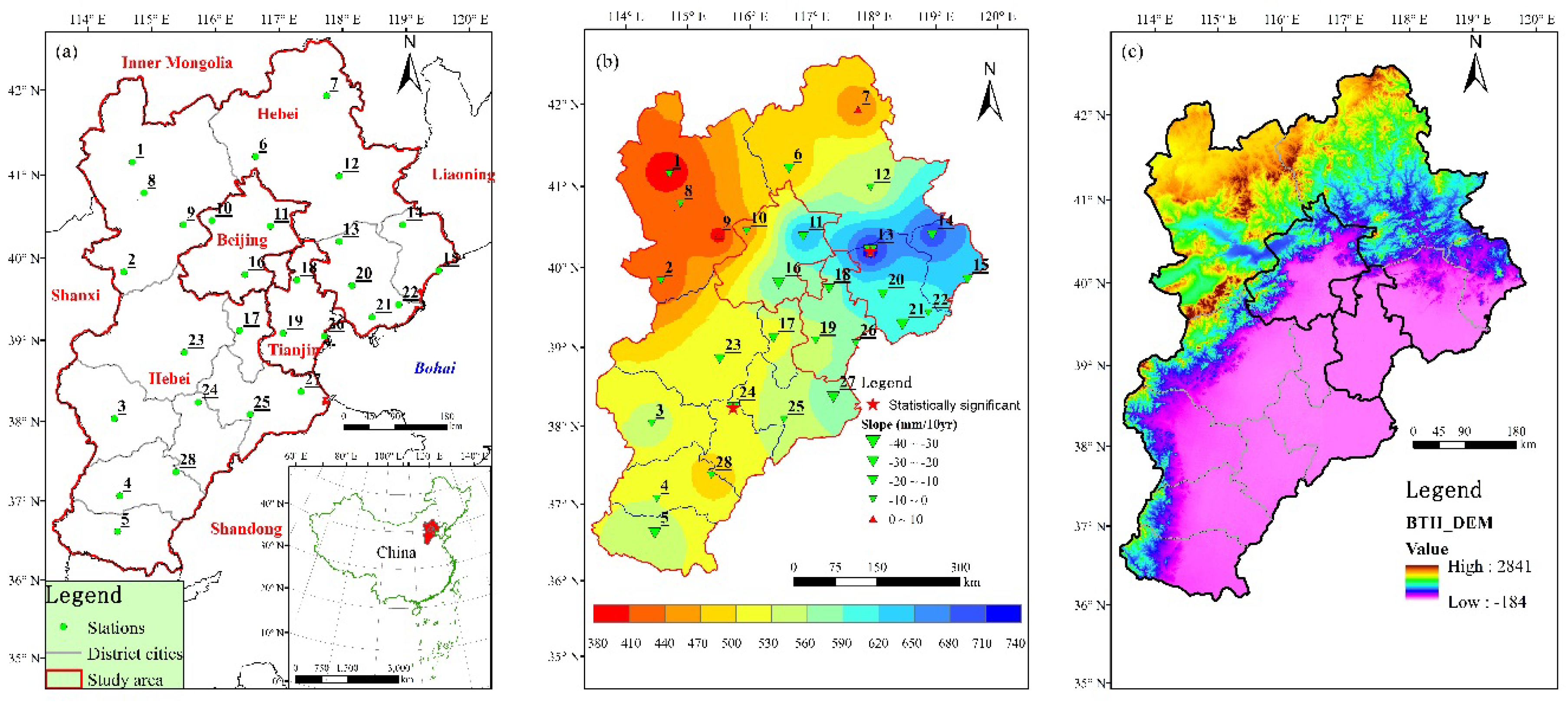
Figure 1. (a) Meteorological stations used for precipitation data in this study. The meteorological stations noted as the number are listed in Table 1. (b) Annual mean precipitation spatial distribution during the period of 1958–2017. The trends and slopes were calculated by the linear regression method, with the significant changes filled red five stars at 0.05 level. (c) Digital elevation model (DEM) data in the study area. DEM data set [50] is provided by Geospatial Data Cloud site, Computer Network Information Center, and the Chinese Academy of Sciences.
Atmosphere 10 00462 g001
Figure 2. Spatial distribution of annual averaged extreme indices in Beijing-Tianjin-Hebei (BTH) during 1958–2017. (unit for PRCPTOT, R × 1day, R × 5day, R95p, and R99p: mm per year; unit for SDII: mm/day per year; unit for consecutive dry days (CDD), consecutive wet days (CWD), R10, R20, R25, and R50: Days per year).
Atmosphere 10 00462 g002
Figure 3. Regional annual averaged time series for all the extreme precipitation indices during 1958–2017. Red lines represent the linear trend of the time series.
Atmosphere 10 00462 g003
Figure 4. Spatial distribution of Mann-Kendall (MK) test results for precipitation extremes in BTH region during 1958–2017. SSD means statistically significant decreasing at the 5% level, while NSD and NSI represent non-significant decreasing and increasing trend, respectively. NT means no any change trend.
Atmosphere 10 00462 g004
Figure 5. Spatial distribution of decadal trend rate for precipitation extremes during 1958–2017 using linear regression method. Upward (red) and downward (green) triangles indicate positive and negative trends, respectively. Triangles are scaled according to trend magnitude. Significant changes at the 5% level are indicated by filled black five stars. Open circle means no any change trend.
Atmosphere 10 00462 g005
Figure 6. Time series of monthly (a,b) and seasonal (c,d) precipitation extremes in R×1day (a,c) and R × 5day (b,d) in BTH during the period of 1958–2017. The regional trends (e) and statistical results for all the stations (f) in monthly and seasonal precipitation extremes using the Mann-Kendall test. NT means no trends, SD and SI mean significantly decreasing or increasing trends, and NSD and NSI mean non-significantly decreasing or increasing trends, respectively.
Atmosphere 10 00462 g006
Figure 7. Box-plots of anomaly percentages for decadal-averaged precipitation extremes from 1958 to 2017 (from left to right: 1958–1967, 1968–1977, 1978–1987, 1988–1997, 1998–2007, and 2008–2017). The upper and lower limits of the box indicate the 75th and 25th percentile value among these stations. The horizontal line in the box indicates the median and the whiskers show the range of these stations. Black solid squares are the mean values of all the stations, connected by the red lines. Open circles represent the outliers.
Atmosphere 10 00462 g007
Figure 8. Decadal variability of extreme precipitation indices from 1958 to 2017 (1958–1967, 1968–1977, 1978–1987, 1988–1997, 1998–2007, and 2008–2017). The decadal precipitation extremes were computed as the average value over each 10-year period.
Atmosphere 10 00462 g008aAtmosphere 10 00462 g008b
Figure 9. Continuous wavelet power spectrum (left panel) and global wavelet spectrum (right panel) of time series of regional average precipitation extremes over the BTH region. The thick black contours designate the 95% confidence level of local power against red noise, and the cone of influence (COI) where edge effects might distort is shown as the dashed U-shape line. The dashed line in the global wavelet power spectrum is the 5% significance level, using a red-noise background spectrum test.
Atmosphere 10 00462 g009
Figure 10. Scale-average wavelet power over the 2–4 years, 4–8 years, and 8–16 years scale bands for precipitation extremes: (a) CDD, (b) CWD, (c) PRCPTOT, (d) R10, (e) R20, (f) R25, (g) R50, (h) R95p, (i) R99p, (j) R×1day, (k) R×5day, and (l) SDII. The dashed line is the 95% confidence level assuming red noise.
Atmosphere 10 00462 g010
Figure 11. Scatter matrix and correlation coefficients of regional annual precipitation and the extreme precipitation indices in BTH from 1958 to 2017. Bold font means the value is statistical significance at a level of α = 0.05.
Atmosphere 10 00462 g011
Figure 12. Spearman’s rank correlation coefficients between extreme precipitation indices and atmospheric circulation indices for each station during 1958–2017. Filled stripes mean the positive or negative correlation coefficients with statistical significance at 5% level.
Atmosphere 10 00462 g012
Figure 13. Spearman’s rank correlation coefficients between (a) monthly R × 1day, (b) monthly R × 5day, and (c) seasonal R × 1day and R × 5day, and atmospheric circulation indices during 1958–2017. Black dashed lines mean the positive or negative correlation coefficients with statistical significance at 5% level.
Atmosphere 10 00462 g013
Figure 14. Correlations in the annual trend magnitudes between the extreme precipitation indices and annual total precipitation (ATP).
Atmosphere 10 00462 g014
Table 1. Geographical coordinates of the weather stations.
No.Station CodeStation NameLatitude (N)Longitude (E)Elevation (m)
153399Zhangbei41.15 114.70 1393.3
253593Yuxian39.83 114.57 909.5
353698Shijiazhuang38.03 114.42 81
453798Xingtai37.07 114.50 77.3
553892Handan36.62114.4766.6
654308Fengning41.22 116.63 661.2
754311Weichang41.93 117.75 842.8
854401Zhangjiakou40.78 114.88 724.2
954405Huailai40.40 115.50 536.8
1054406Yanqing40.45 115.95 489
1154416Miyun40.38 116.87 71.8
1254423Chengde40.98 117.95 385.9
1354429Zunhua40.20 117.95 54.9
1454436Qinglong40.40 118.95 227.5
1554449Qinhuadao39.85 119.52 2.4
1654511Beijing39.80 116.47 31.3
1754518Bazhou39.12 116.38 9
1854525Baodi39.73 117.28 5.1
1954527Tianjin39.08 117.07 2.5
2054534Tangshan39.67 118.15 27.8
2154535Caofeidian39.28118.473.2
2254539Laoting39.43 118.88 10.5
2354602Baoding38.85 115.52 17.2
2454606Raoyang38.23 115.73 19
2554618Botou38.08 116.55 13.2
2654623Tanggu39.05 117.72 4.8
2754624Huanghua38.37 117.35 6.6
2854705Nangong37.37 115.38 27.4
Table 2. Expert Team on Climate Change Detection and Indices (ETCCDMI) precipitation-related extreme indices used for this study.
Acronym.DefinitionUnit
R10Annual number of days with more than 10 mm/daydays
R20Annual number of days with more than 20 mm/daydays
R25 *Annual number of days with more than 25 mm/daydays
R50 *Annual number of days with more than 50 mm/daydays
CDDMaximum number of consecutive dry days 1days
CWDMaximum number of consecutive wet days 2days
R95pAnnual total precipitation when daily precipitation >95th percentilemm
R99pAnnual total precipitation when daily precipitation >99th percentilemm
R × 1dayAnnual, seasonal and monthly maximum one-day precipitationmm
R × 5dayAnnual, seasonal and monthly maximum five-days precipitationmm
SDIIAnnual total precipitation divided by the number of wet days in the yearmm/d
PRCPTOTAnnual total amount of precipitation cumulated in wet daysmm
* 25 mm and 50 mm were the thresholds defined by the authors. 1 Dry days are those days when daily precipitation was < 1 mm; 2 Wet days are those days when daily precipitation was ≥ 1 mm.
Table 3. Results of the statistical tests for regional extreme precipitation indices and the number of stations with positive or negative trends over the BTH region from 1958 to 2017.
IndexMann-Kendall Trend TestLinear Regression Trend
Z ScorePositiveNegativeNo TrendSlope of Change (b)p ValuePositiveNegativeNo Trend
TTSSTTSSTTSSTTSS
CDD−0.778402420−0.1430.3371001800
CWD−1.843302520−0.0070.06302560
PRCPTOT−0.887502320−1.0270.183202620
R100.0701501300−0.0090.684802000
R20−0.472602101−0.0120.377402400
R25−0.619602101−0.0130.261402331
R50−2.398702130−0.010.025302253
R95p−2.137602230−0.850.041502340
R99p−2.749702130−0.4780.036502350
R×1day−3.042502330−0.2650.022402430
R×5day−2.532502340−0.5050.021302550
SDII−0.874802010−0.0090.361801911
TT, total number of stations with positive or negative trends; SS, statistically significant at the 0.05 level. Bold font for Z score or slope of change (b) means the statistically significant at a level of 0.05.
Table 4. Spearman’s rank correlation coefficients between regional extreme precipitation indices and climate variables and the number of stations for positive or negative correlation coefficient between precipitation extremes and climate variables.
IndicesNAO-1NAO-0NINO3.4-1NINO3.4-0PDO-1PDO-0
CDD−0.1320.135−0.3730−0.152−0.208
CWD0.03−0.20.2730.0340.2040.038
PRCPTOT0.09−0.1230.379−0.1530.074−0.067
R100.111−0.0380.397−0.130.1290.005
R200.128−0.1030.337−0.1830.076−0.095
R250.11−0.1080.336−0.180.067−0.109
R50−0.026−0.217*0.251−0.181−0.089−0.201
R95p0.012−0.213*0.254−0.247*−0.04−0.2
R99p0.019−0.235*0.122−0.236*0.093−0.152
R × 1day−0.016−0.229*0.205−0.223*0.039−0.198
R × 5day0.082−0.1880.222*−0.2580.052−0.152
SDII0.064−0.190.295−0.3290.065−0.142
Note: Correlation coefficients significant at 5% level are bolded. The mark * represents the significant correlation at 10% level.
Table 5. Spearman’s rank correlation coefficients between the decomposed series of extreme precipitation indices and climate variables.
IndicesNINO3.4-0NINO3.4-1
2-year4-year8-year16-year2-year4-year8-year16-year
CDD0.396−0.382−0.255−0.479−0.565−0.336−0.512−0.483
CWD−0.2090.0630.334−0.2240.2670.2080.362−0.240
PRCPTOT−0.325−0.0670.245−0.5460.4660.0450.165−0.519
R10−0.3260.1000.390−0.6560.4120.2540.469−0.614
R20−0.291−0.0270.275−0.6740.4520.0370.304−0.638
R25−0.245−0.1030.304−0.5910.416−0.0140.251−0.569
R50−0.243−0.2740.020−0.6070.348−0.159−0.144−0.618
R95p−0.341−0.3060.008−0.3550.491−0.160−0.147−0.380
R99p−0.140−0.4700.0090.2000.200−0.204−0.0600.143
R×1day−0.260−0.531−0.1740.0700.281−0.018−0.1630.021
R×5day−0.112−0.400−0.036−0.1960.3210.098−0.177−0.232
SDII−0.222−0.3040.170−0.6910.3680.0320.190−0.715
IndicesNAO-0NAO-1
2-year4-year8-year16-year2-year4-year8-year16-year
CDD0.0970.3760.0150.705−0.208−0.0170.2870.561
CWD−0.377−0.219−0.2240.2780.2760.1790.2080.368
PRCPTOT−0.212−0.065−0.3090.6260.3340.3210.0970.569
R10−0.207−0.083−0.2620.6530.3010.2090.1260.554
R20−0.188−0.065−0.2870.6780.2500.3070.1460.592
R25−0.1940.014−0.3010.6810.2200.3500.1230.586
R500.0260.017−0.3140.602−0.0230.4410.0470.633
R95p−0.1100.038−0.3210.4880.0710.4150.0720.527
R99p−0.3660.1510.1270.1100.2250.3600.4230.207
R×1day−0.3330.3550.0760.1550.2380.4140.4190.242
R×5day−0.3230.2070.0980.2850.2770.4300.4270.410
SDII0.2700.193-0.1010.7020.0930.3950.3310.746
IndicesPDO-0PDO-1
2-year4-year8-year16-year2-year4-year8-year16-year
CDD−0.051−0.306−0.122−0.593−0.0550.184−0.363−0.707
CWD−0.4360.1390.6660.1170.562−0.1290.628−0.083
PRCPTOT−0.074−0.1160.514−0.5380.339−0.1520.420−0.668
R10−0.0880.0340.709−0.7530.330−0.1000.706−0.828
R20−0.120−0.1290.614−0.7090.324−0.2060.581−0.813
R25−0.166−0.1900.583−0.6520.365−0.2080.475−0.770
R50−0.046−0.3330.263−0.3410.178−0.2050.129−0.565
R95p−0.110−0.3160.276−0.0510.355−0.1670.154−0.290
R99p−0.208−0.3080.3870.6290.4590.0150.2470.415
R×1day−0.239−0.3200.2710.4480.4990.1060.2320.232
R×5day−0.106−0.1930.2620.2800.4220.0620.1010.047
SDII−0.244−0.2480.568−0.2840.442−0.0740.490−0.553
IndicesIOD-0IOD-1
2-year4-year8-year16-year2-year4-year8-year16-year
CDD−0.2730.1910.0290.939−0.396−0.0170.4880.925
CWD0.015−0.217−0.2660.0780.0080.435−0.1960.027
PRCPTOT−0.018−0.210−0.2350.5980.2060.404−0.0520.569
R10−0.064−0.188−0.3680.6890.2620.422−0.3530.691
R200.027−0.153−0.2320.6990.3030.417−0.1490.698
R250.104−0.117−0.2920.7480.2520.433−0.1410.727
R500.115−0.2110.0930.5060.1300.4140.2290.489
R95p0.024−0.1470.0430.3850.1600.4230.2390.334
R99p0.001−0.0990.358−0.086−0.0470.4000.451−0.158
R×1day0.0470.1360.469−0.0060.0330.6390.525−0.078
R×5day0.0480.0780.3290.0110.0140.7040.442−0.028
SDII0.1080.0730.0470.5390.2470.6170.1020.545
Note: Correlation coefficients significant at 5% level are bolded.