Abstract
In ultrasonic equipment (anemometers and thermometers), for the measurement of parameters of atmospheric turbulence, a standard algorithm that calculates parameters from temporary structural functions constructed on the registered data is usually used. The algorithm is based on the Kolmogorov–Obukhov law. The experience of using ultrasonic meters shows that such an approach can lead to significant errors. Therefore, an improved algorithm for calculating the parameters is developed, which allows more accurate estimation of the structural characteristics of turbulent fluctuations, with an error that is not more than 10%. The algorithm was used in the development of a new ultrasonic hardware-software complex, autonomous meteorological complex AMK-03-4, which differs from similar measuring instruments of turbulent atmosphere parameters by the presence of four identical ultrasonic anemometers. The design of the complex allows not only registration of the characteristics of turbulence, but also measurement of the statistical characteristics of the spatial derivatives of turbulent temperature fluctuations and orthogonal components of wind speed along each of the axes of the Cartesian coordinate system. This makes it possible to investigate the space–time structure of turbulent meteorological fields of the surface layer of the atmosphere for subsequent applications in the Monin–Obukhov similarity theory and to study turbulent coherent structures. The new measurement data of the spatial derivatives of temperature at stable stratification (at positive Monin–Obukhov parameters) were obtained, at which the behavior of the derivatives was been investigated earlier. In the most part of the interval of positive Monin–Obukhov parameters, the vertical derivative of the temperature is close to a constant value. This fact can be considered as a new significant result in similarity theory.
1. Introduction
The first acoustic thermometers and anemometers were used for experimental research in the field of atmospheric physics in the 1950s as single devices and developments [1,2,3,4]. Today, with the development of electronic technology and microprocessor technology, ultrasonic anemometers are manufactured industrially and are increasingly used. The measurement process is automated and includes simultaneous measurements of many parameters of the turbulent atmosphere.
At the moment, there are many modifications of such ultrasonic acoustic systems of various designs with different measurement errors and sensitivity, with different sampling frequencies and measurement ranges of turbulent atmosphere parameters.
A description of various ultrasonic measuring instruments, anemometers, and thermometers has been provided in the literature [5,6,7,8,9]. A detailed review of existing ultrasonic anemometers is given in [5]. Ultrasonic meters are often used for the study of meteorological fields in the surface layer of a turbulent atmosphere, which implies the coupling of an ultrasonic system with a computer and the availability of software developed in accordance with the objectives of meteorological research.
The known main advantages of ultrasonic anemometers are their ability to measure instantaneous values of the measured characteristics of a turbulent atmosphere (low inertia) with high sampling rates (up to 100 Hz or more), the practical absence of distortion in the measured air flow due to the details of its own design, and the obtainment of a large amount of data on measured and calculated parameters in real time. The principle of operation of ultrasonic meteorological systems is to measure the delay time, ∆t, for the passage of the acoustic signal between pairs of ultrasonic transducers (sensors) spaced at known distances S: ∆t = S/(c + v), where c is the speed of sound and v is the speed of air movement between the sensors.
This paper presents a new ultrasonic hardware-software complex, AMK-03-4, the design of which allows registration of the statistical characteristics of spatial derivatives of turbulent fluctuations. Algorithms of the calculation correction of measurement errors arising in ultrasonic systems are presented.
Measurements and calculation of atmospheric turbulence parameters, as well as the construction of power spectra and structural functions (and other features), are standard functions of the software used by us ultrasonic complexes. Qualitatively, the measurement results of the new complex AMK-03-4, as expected, differ little from our previous measurements made using simpler ultrasonic anemometers. Complex AMK-03-4 is a development of complex AMK-03 previously used by us with one measuring sensor. Therefore, in this article, we only aim to discuss the issues of the calibration of ultrasonic devices, based on our extensive experience of measurements (including setting up a new AMK-03-4 complex).
In general, our article is devoted to technical aspects of functioning of ultrasonic meters of turbulent atmosphere parameters and the processes of their calibration. The results in the article are the algorithms for calculating the turbulence parameters and the calibration algorithms for meters to eliminate systematic errors.
Direct data on measurements of the parameters of the turbulent atmosphere (including data on measurements of spatial derivatives) are contained, for example, in our papers [10,11,12] and in the papers of other authors [13,14]. For example, in the studies of 2011 [11], we developed a numerical regularization algorithm for the restoration of spatial derivatives of the mean temperature from long samples of experimental data obtained in the atmospheric anisotropic boundary layer. The algorithm is based on the solution of the thermal conductivity equation taking into account the relations of the semi-empirical theory of turbulence. The found average derivatives allowed the the dependence of the Prandtl turbulent number on the Monin–Obukhov parameter, ζ, to be stablished.
2. Equipment, Data, and Methods
2.1. Recorded Meteorological and Statistical Data
2.1.1. Ultrasonic Complex AMK-03
In our measurements of atmospheric parameters in the surface layer, we used the autonomous meteorological complex, AMK-03 [15,16,17,18], and its new modification, AMK-03-4 [19] (Figure 1). The maximum measurement frequency (sampling) of the AMK-03 complex is 160 Hz.
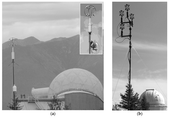
Figure 1.
Appearance of the ultrasonic meteorological complexes AMK-03 (a) and AMK-03-4 (b).
The AMK-03 complex registers six meteorological parameters and calculates in real time more than 100 statistical parameters of atmospheric turbulence. The recorded meteorological parameters include air temperature, the three orthogonal components of the wind velocity vector (and the horizontal wind direction), atmospheric pressure, and relative air humidity. They are stored in the computer’s RAM (random access memory) for the time interval equal to the set averaging time, counted back from the moment of receipt of the last information package from the device. That is, there are always arrays of instantaneous values of meteorological parameters with a large number of their elements (averaged over 10 min, the sample has 48,000 elements). The software in the time and observation periods specified by the operator calculates from these arrays the average values of meteorological parameters and their other statistical moments, as well as the standard numerical characteristics of atmospheric turbulence, automatically storing the results in text files. The main calculated characteristics of turbulence include the heat and impulse flows, scale of temperature (T*) and wind (V*) fluctuations, the scale and Monin–Obukhov’s length, and also the structural characteristics of temperature fluctuations, CT2 (deg2 cm−2/3), of the longitudinal component of wind speed, CV2 ((m/c)2 cm−2/3), of the acoustic refraction index, Cna2 (m−2/3), and of the optical refraction index, Cn2 (cm−2/3).
The output data of the measurements of the AMK-03 complex are partially (only the values of the primary data of ultrasonic anemometers and the basic meteorological parameters) displayed on the monitor screen in the main window of the AMK-03 software. Much more diverse information is written to files on the computer’s hard drive. The program records 16 different files of different types with registered and calculated real-time instantaneous and averaged data on the hard disk in one measurement session. Also, a summary file with a table of rows with different measurement sessions with all the measured averaged data is also recorded.
2.1.2. The Modified Complex AMK-03-4 with Four Ultrasonic Anemometers
In the last modification of the ultrasonic complex AMK-03-4 [19], the complex includes four identical ultrasonic anemometers with a measurement frequency, Fd = 80 Hz, spaced 30 to 35 cm in the orthogonal directions (Figure 2).
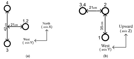
Figure 2.
The scheme of spatial placement in the complex AMK-03-4 of ultrasonic measuring heads UGI-75 with serial numbers 1, 2, 3, and 4: (a) top view; (b) side view in the direction of north.
Due to this design, ultrasonic measurements of turbulent fluctuations are made simultaneously in four spatially separated areas of atmospheric air. Due to this, there is a unique opportunity to evaluate not only the standard parameters of atmospheric turbulence in each of the measurement areas separately but also the statistical characteristics of instantaneous spatial derivatives of turbulent fluctuations along each of the axes of the Cartesian coordinate system.
In the modified complex AMK-03-4, registration of the statistical characteristics of instantaneous spatial derivatives of turbulent temperature pulsations and orthogonal components of wind speed, as well as derivatives of pressure and relative humidity are implemented, which is the main difference between the complex AMK-03-4 and the commercially produced weather station AMK-03 and other similar ultrasonic devices.
This allows an investigation of the spatial-temporal structure of turbulent meteorological fields for subsequent applications in the Monin–Obukhov similarity theory and the study of coherent structures in the turbulent atmosphere.
The compound structure of the components of the complex AMK-03-4 and their functional interaction can be seen in Figure 3. When you turn on the power supply, it outputs a constant voltage of 12 V to the collector and further from it to each of the UGI-75 ultrasonic anemometers. In the presence of power, the UGI-75 anemometers automatically perform the measurements necessary for the calculation of all estimated meteorological parameters, repeating them with a sampling frequency (sample rate) of Fd = 80 Hz. The primary data of their measurements, with a periodicity in time equal to 1/Fd, comes to the collector as digital information packets in the RS485 standard at a speed of 57,600 bps. The combined packets are fed into the power supply, also with a repetition rate of 80 Hz and in the RS485 standard but already at a higher speed of 115,200 bps. In the power supply, they are converted in such a way that they can already be read by the software (Figure 4) in the computer through any available USB (universal serial bus) port.
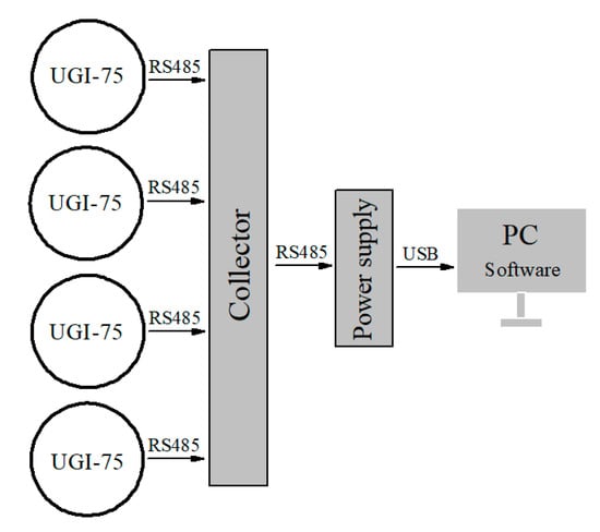
Figure 3.
The structural scheme of the complex AMK-03-4.

Figure 4.
Main window of the “AMK-rotor” program.
The estimation of measurement errors of space derivatives using the AMK-03-4 complex can be obtained by using average characteristics and Monin–Obukhov similarity theory (MOST). Let us estimate the relative error of measurements of vertical derivatives of average meteorological parameters.
The parameters, z2, z1, are, respectively, the upper and lower heights of the measuring sensor, and T(z) is the average air temperature. The meter finds the value:
D = [T(z2) − T(z1)]/(z2 − z1).
By placing T(z2) in the Taylor row, we get:
T(z2) = T(z1 + ∆z) = T(z1) + [dT(z1)/dz1] ∆z + (1/2) [d2T(z1)/dz12](∆z)2 + …, ∆z = z2 − z1.
Substituting T(z2) into D, we have:
D = dT(z1)/dz1 + (∆z/2) d2T(z1)/dz12 + …
Provided that the derivatives of higher orders are small in comparison with the derivatives of the first order (this is actually observed in experiments), the relative error, E, of measurement of the derivative, dT(z1)/dz1, can be represented in the form:
E = |(D − dT(z1)/dz1)/(dT(z1)/dz1)| ≈ ∆z/2|(d2T(z1)/dz12)/(dT(z1)/dz1).
Monin–Obukhov similarity theory describes the average vertical derivatives of the first order of the temperature, T, and longitudinal velocity, u, by the formulas:
where T* and V* are the turbulent temperature and velocity scales, ζ = z/L is the Monin–Obukhov parameter, T* is an analogue of the turbulent velocity scale (friction velocity) (V*), L is the Monin–Obukhov length (scale), æ = 0.4 is the von Karman constant, and φ(ζ) is a universal function of similarity that specifies the type of stratification.
E = |(D − dT(z1)/dz1)/(dT(z1)/dz1)| ≈ ∆z/2|(d2T(z1)/dz12)/(dT(z1)/dz1)|,
dT/dz = [T*/z] φ(ζ), du/dz = V* φ(ζ)/(æ z),
In MOST, it is accepted that T* and V* changes weakly with height. This condition is one of the main MOST postulates (axioms). Therefore, both dT*/dz and dV*/dz vary slightly with height.
There are various scientific views on the function, φ(ζ). We adhered to the approach of Tatarsky V.I. [20] and Monin A.S., Yaglom A.M. [13,14]. Within these views, φ(ζ) is a quantity that also weakly varies with the height, like its derivative by z.
Therefore, the derivatives, dT*/dz and dφ/dz, can be neglected further compared to T* and φ; also the derivatives, dV*/dz and dφ/dz, can be neglected compared to V* and φ. In order to further simplify the result, we next considered a neutral stratification, for which, as is known, ζ → 0 (L → ∞) and φ(ζ) ≈ 1.
By differentiating, we find the relative error of measurements by the vertical derivative of the mean temperature, T:
E = (∆z/2)|(−T*/z2)/(T*/z)| = ∆z/(2z).
A similar formula is obtained for the relative measurement error of the vertical derivative of the mean longitudinal velocity, u.
These formulas show that, in the case of neutral stratification in the ground layer, the relative error, E, of the measurements of the mean vertical derivatives, T and u, is approximately ∆z/(2z), where ∆z is the vertical distance between anemometers and z is the height of the measuring sensor above the underlying surface. Therefore, for example, for ∆z = 35 cm (as is customary in AMK-03-4), and z = 2.5 m (near the surface), the relative error of measurements by a vertical derivative (both temperature, T, and longitudinal velocity, u) does not exceed 7%. As can be seen, E decreases with the height, z, above the underlying surface. Therefore, E = 3.5%, for example, at a height of z = 5 m.
2.2. Basic Errors and Sensitivity of Ultrasonic Anemometers: Experimental Methods
Let us consider the systematic errors of the measurement of ultrasonic anemometers on the example of the complex AMK-03 [15,16,17,18]. Systematic errors are determined by the technical capabilities of graduation of the anemometers included in the complex and for the main averaged parameters in AMK-03, they do not exceed: 0.3 °C for temperature; 0.15 m/s for wind speed vector components; 0.4 mm Hg for pressure; and 2.5% for relative humidity.
The specified systematic errors of measurements of temperature and wind speed can be more than an order of magnitude higher than the achieved threshold sensitivity, σT (on temperature) and σV (on velocity), of the ultrasonic anemometer to turbulent fluctuations. It is caused by the essential prevalence in similar devices of systematic errors over random errors of measurements. In [18], engineering formulas for the estimation of σT and σV are given:
where q = 1/f is a unit of quantization of the measured time intervals in ultrasonic anemometers (their digital resolution), the T-value of air temperature in Kelvin, and S-distance between ultrasonic sensors. The values of the threshold sensitivity for the frequency of piezoceramic sensors, f = 72 MHz and S = 0.07 m, are specified in Table 1 at three different values of T.
σT ≈ 10 q T3/2/S, σV ≈ 200 q T/S,

Table 1.
Threshold sensitivity of measurements of temperature and wind speed.
The used frequency of sampling of instantaneous values of temperature and wind speed components, for example, equal to fd = 80 Hz, leads to the cutoff of frequencies of a large 40 Hz in the estimated spectra of their turbulent fluctuations. Therefore, such an ultrasonic complex does not feel turbulent inhomogeneities whose dimensions are less than <v>/fd (for example, at an average wind speed <v> = 3 m/s, it is less than 4 cm). This fact does not affect measurements of temperature fluctuations and wind components from the inertial interval of the frequencies of atmospheric turbulence to the synoptic range but limits the possibility of an experimental study of small-scale turbulence components at higher frequencies (in the viscous turbulent interval). For a guaranteed capture of the smallest sizes of inhomogeneities of air (up to less than 1 cm) at usual average wind speeds (up to 5 m/s), it is required that the frequency of measurements, fd, is raised to 500 Hz. At the same time, this practically does not affect the accuracy of measurements of random characteristics of meteorological fields. Thus, the results of direct measurements of the turbulence spectra show that when registering the random temperature and wind speed, the error value introduced by the value, fd = 80 Hz, usually does not exceed 1%. This is due to the small contribution of the cutoff portion of the spectrum to the total energy of turbulent fluctuations.
When measuring turbulent parameters, the averaging time (random sampling length) is selected from the condition that the length scale of the averaged turbulent flow (average wind speed multiplied by the averaging time) significantly exceeds the turbulence outer scale in the direction of the average flow (or the averaging time should greatly exceed the characteristic time scale of correlation of the studied fields, according to the ergodic theorem of Taylor [13,14,20]). Then, the time averages will be statistically stable. Measurements in the atmospheric surface layer over a smooth surface are usually produced with the averaging time of at least (or of the order) 100 s [13,14,20]. The length scale corresponding to this time for the wind speed of 1 to 10 m/s is 0.1 to 1 km and exceeds the turbulence outer scale (which is usually not more than 10 meters near the underlying surface [13,14,20]).
In the case of an uneven surface, the longitudinal outer turbulence scale in the lower surface layer will obviously be determined by the characteristic distance between the roughness or surface inhomogeneities. For a mountain relief with a non-uniform surface, such a near-surface distance is small, and can be estimated by tens of meters. Therefore, for uneven surfaces, the measurements in the surface layer can be made with averaging time of about 100 s [10,11].
When measuring indoors, the outer scale of turbulence is limited by the room size. However, in reality, it is significantly (5–10 times [10,11,12]) smaller than these sizes. For an averaging time of 100 s and typical wind speed of 0.05 to 0.5 m/s, the length scale is 5 to 50 m and exceeds the outer scale observed in the premises. Therefore, in closed rooms, measurements can also be made with an average of 100 s.
As shown in [13,14,20], when measuring turbulent parameters, it is sufficient that the interval of the fluctuation frequencies recorded in the measurements overlap for the most part of the so-called micrometeorological maximum of the atmospheric turbulence spectrum. It is in this micrometeorological interval that the main energy of turbulent fluctuation is concentrated. The lower border of the micrometeorological maximum is usually located approximately near the frequency of 0.01 Hz [13,14,20], which corresponds to the averaging time of 100 s. Therefore, for the normal averaging time, when recording the turbulence parameters by ultrasound complexes, it usual takes t = 120 s. During this averaging time at a measurement frequency, fd = 80 Hz, the number of samples is N = 9600 (N = taver fd), with an interval between them, ∆t = 1.25 × 10⁻² s. In measurements of lower frequency (than turbulent) meteorological parameters associated with daily and seasonal changes in the meteorological situation, the width of one micrometeorological interval is often not enough, and it is necessary to increase the averaging time to 10 min or more (by expanding the interval of frequencies recorded in the measurements in the region of a lower-frequency synoptic maximum [13,14,20]).
The relative accuracy of measurements of the structural turbulent characteristics, CT2, CV2, Cn2, is defined, first of all, by the threshold sensitivity of the device and decreases with an increase in the average wind speed, averaging the time and values of structural characteristics. For example, in the conditions of rather weak turbulence (Cn2 = 5 × 10⁻¹⁶ cm−2/3), at the averaging time 2 min and the average wind speed of 0.5 to 10 m/s, the relative accuracy of measurements of the value Cn2 is in range of 0.4% to 14% (0.4%, 7%, and 14%, respectively, for the wind speeds of 10, 1, and 0.5 m/s). With the same errors, characteristics, CT2 and CV2, are also measured. The dissipation speeds of the kinetic energy, ε, and temperatures, N, are taken on the basis of Kolmogorov–Obukhov’s law. Therefore, the relative accuracy of measurements, ε (N), is practically the sum of errors, CV2, and Kolmogorov’s constant, C (CT2 and Obukhov’s constant, Cθ, for the dissipation speeds of temperatures, N).
3. Results
3.1. Algorithm of the Registration of Structural Characteristics of Turbulent Fluctuations and Measurement Error
The standard algorithm for calculating the structural characteristics of CT2, CV2, Cn2, usually used in ultrasonic measuring equipment for studying the turbulent properties in the surface layer of the atmosphere, is based on the Kolmogorov–Obukhov law for structural functions. In calculating the structural characteristics, the existing calculation algorithm under some meteorological conditions of observations leads to measurement errors. The problem with the calculation algorithm is due to high measurement frequencies in ultrasonic systems. With a small amount of time separation between the measurements and at low wind speeds, it is possible to be at the boundary of applicability of the Kolmogorov–Obukhov law outside the inertial interval of atmospheric turbulence, where a different behavior of the structural function is observed. On Figure 5, a graph of one of the experimental structural functions of temperature fluctuations, D′T (τ), (solid line) is given, and the insert shows an enlarged initial section of this function. It is seen that at the initial site with a small separation, τ, the behavior of the structural function, D′T (τ), differs from 2/3 of the asymptotic corresponding to the Kolmogorov dependence (dashed line). This corresponds to theoretical representations for the interval of small spatial dimensions up to the inner scale, l0T, of atmospheric turbulence [13,14,20].
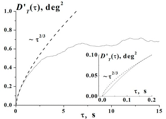
Figure 5.
The experimental structure function of temperature fluctuations of D′T (τ) (solid line). In the inset at the lower right, its initial part is increased with a small separation, τ, showing behavior different from the Kolmogorov “2/3” asymptotic. Sayan, 19.07.2017.
This can lead to errors in the calculation of structural characteristics when using the existing algorithm. Therefore, for the ultrasonic complex AMK-03-4, a modified improved algorithm for calculation of the structural characteristics is used to avoid the appearance of such errors in the measurements.
The offered improved algorithm consists in the implementation of a more exact choice of the argument of structural functions of fluctuations of temperature and speed. Both the temporary, D′, and space, D, structural functions of fluctuations connected owing to the Taylor “frozen turbulence” hypothesis by equality D′(τ) = D(v τ) are for this purpose used, where τ is the time spacing and v is the vector of the average speed of wind. The value of the spacing, τ, has to provide a sure hit of the argument of the structural function in the area of the “2/3” asymptotic of the structural function in which Kolmogorov–Obukhov’s law is fulfilled. This law for fluctuations of the temperature, T, for example, has an appearance, D′T (τ) = DT(v τ) = CT2 τ2/3 (CT2 = D′T (τ)/(v τ) 2/3) [13,14,20], where DT′(τ) = <[T(t + τ) − T(t)]2>.
In the calculated algorithm, the time interval, τ, has to be such that the condition, (v τ) >> l0T, is realized (or τ >> l0T/v, l0T is the temperature inner scale of turbulence), as at the smaller scales of the estimated turbulence, other behavior of the structural function is observed (D′T (τ)~τ2 [13,14,20]). This condition in measurements by ultrasonic systems with a high frequency of taking samples, f = 1/τ, may not be fulfilled, which often leads to considerable errors of measurements.
As the calculations of the structural function (for the existing turbulence spectrum models) show, in Kolmogorov turbulence, with the accuracy sufficient for practice, inequality, τ >> l0T/v, can be replaced with inequality:
where as the inner scale of temperature turbulence, l0T, it is necessary to use its maximum value, l0T max (see Equation (13)).
τ ≥ τb, τb = w l0T/v, w = const, w > 1,
Calculation shows that the constant, w, in Equation (9) depends both on the inner scale of turbulence and on the outer scale. For the finite sizes of the outer scale of turbulence (near-surface measurements), an accuracy of measurements of 100%, CT2, from the Kolmogorov–Obukhov’s law, owing to its asymptotic nature, is never reached.
If the outer scale of turbulence uses the most simply evaluated outer scale of the Tatarski V.I. L0T [20], then at l0T = l0T max and small values of scale L0T, for example, for L0T = 1 m (that corresponds to measurements at the height of 2.5 m from the underlying surface), the constant, w, can be chosen to equal w = 14. At the same time, the error of measurements, CT2, will not exceed 10% (that corresponds to a reduction of the measured value, CT2, in comparison with the true value no more, than for 10%). At w = 28, the error of measurements, CT2, will exceed 7%. A further increase in the constant, w, however, will not lead to a reduction of the error of measurements, CT2. The error will only grow. Therefore, for L0T = 1 m, the minimum error of measurements, CT2, is 7%.
At the smaller sizes of the outer scale (L0T < 1 m, measurements in the enclosed space), for a reduction of the error of measurements, CT2, it is necessary to reduce the constant, w (getting closer to a value of w = 14) while the minimum error of measurements remains more than 10%.
The case of the big sizes of the outer scale of turbulence, which is implemented in measurements at heights more than 2.5 m from the underlying surface, is more optimistic. With growth of the outer scale, the minimum error of measurements, CT2 (at the same pre-defined constant value, w), decreases. For example, at the height of 10 m (L0T = 4 m) and w = 14, the error decreases from 10% to 9%. However, at the same height of 10 m at w = 72, the minimum error is already 4%. Therefore, in case of enough big heights of measurements (not less than 10 m), it is possible to take for the constant, w, its value of w = 72 and to consider that the minimum error of measurements, CT2, is 4%.
In view of the observations and considering that ultrasonic meteorological systems are intended generally for near-surface measurements, we further consider the constant, w, equal to w = 14. The minimum error of measurements, CT2, on the basis of Kolmogorov–Obukhov’s law can then be considered equal to 10%.
Size τb in Equation (9) can be considered as the lower limit (lower bound) for the temporary spacing, τ, providing (at τ ≥ τb) applicability of the Kolmogorov asymptotes of the structural function, D′T (τ). The interval, smaller than τb, leads to deviations from the Kolmogorov asymptotes and therefore gives essential errors (reduction of the measured value in comparison with the true value more than for 10%) in the measured value of the structural characteristic, CT2.
It is also necessary to mean that the interval, τ, significantly bigger than τb, can also lead to considerable errors in CT2 as in this case, we can go beyond the applicability of the Kolmogorov asymptotes already from very big τ. As the calculations show, for small outer scales of turbulence, for example, for L0T = 1 m, the interval, τ, has to satisfy inequality:
τ ≤ 120 l0T/v.
At the same time, the error of measurements, CT2, exceeds 10%. With growth of the outer scale, L0T, the right part of Equation (10) (the upper bound of the rating, τ) beyond all bounds increases.
The temperature inner scale of turbulence, l0T, is usually defined [13,14] as the intersection point of two known asymptotes by the structural function, DT(ρ) (initial square and Kolmogorov “2/3”—asymptotes for the space intervals, respectively, less and more l0T). The temperature inner scale, l0T, is connected with the Kolmogorov inner scale of turbulence, l0K, by the formula, l0T = (3 Cθ/Pr)3/4 l0K [13,14,20], where Cθ is a constant of A.M. Obukhov (Cθ ≈ 3.0 [13,14,20]) and Pr is the molecular Prandtl number (for air Pr ≈ 0.7 [13,14,20]). Substituting the values of the constants, we find:
l0T = 6.79 l0K.
In [10,11,12], the experimental results for the Kolmogorov inner scale of turbulence, l0T, received according to the series of measurements in the mountain region are given. In [10,11], it was shown that according to all measurements, the mean value of the Kolmogorov inner scale < l0K > and its maximum value, l0K max, are:
< l0K > = 0.64 mm, l0K max = 1.2 mm.
At the same time, the density of probabilities for the Kolmogorov inner scale is close to logarithmic normal density. Substituting values of Equation (12) in Equation (11), we receive:
< l0T > = 4.35 mm, l0T max = 8.15 mm.
For ultrasonic digital meters, any set time interval, τ, between two set moments of observation is a discrete feature. If ∆t [s] is the time interval between the neighboring measuring points, then τ= N ∆t, where N is some integer number. Number N in the existing widespread algorithm of calculation for ultrasonic anemometers is equal to a unit (N = 1); at the same time, the specified time interval, τ, is fixed and is constantly equal to one sampling time interval, τ = ∆t.
The time interval in any digital meter is τ = N ∆t = N/f. Then:
CT2 = D′T (N ∆t)/(v N ∆t)2/3.
At the same time, from the condition, τ ≥ τb (the Equation (9), in which it is necessary to put τ = N ∆t, l0T = l0T max), it follows that N ∆t ≥ τb. If we present τb in the similar form, τb = nb ∆t, where nb is a real (not necessarily an integer) number, we find τ = N∆t ≥ τb = nb ∆t. It corresponds to inequality N ≥ nb. Thus, number N is the next integer number exceeding the real number:
or equal to it if nb appears as the integer number.
nb = τb/∆t = τb f = w l0T max (f/v),
Substituting in Equation (15) the values, w = 14 and l0T max = 8.148 mm, from Equations (9) and (13), we receive a simpler numerical expression for nb:
nb = 0.11407m (f/v), f [Hz], v [m/s], N ≥ nb,
By means of Equations (15) and (16), it is possible to numerically simplify the denominator of Equation (14):
(v N ∆t)2/3 = [(N/nb) nb v ∆t]2/3 = (N/nb)2/3 (w l0T max)2/3,
= (N/nb)2/3 (11.407 cm) 2/3 = 5.067 (N/nb)2/3 cm2/3,
= (N/nb)2/3 (11.407 cm) 2/3 = 5.067 (N/nb)2/3 cm2/3,
Substituting Equation (17) into Equation (14), we finally find the expression allowing recovery from the near-surface temperature measurements of the value of the structural characteristic, CT2, on the basis of Kolmogorov–Obukhov’s law (with an error of no more than 10%):
CT2 = 0.19734 (nb/N)2/3 < [T(t + N ∆t) − T(t)]2 > K2 cm−2/3.
In algorithms, accounting for the calculation of structural characteristics, CT2 (and also for Cn2, CV2), in Equation (18) leads to a decrease in the error of measurements, which at the same time does not exceed 10%.
In Figure 6, two graphs of three-hour measurements of the structural characteristics of fluctuations of the refractive index, Cn2, by an ultrasonic anemometer, with averaging for two minutes, are given. The registration of Cn2 values was made by one anemometer simultaneously with the use of usual (light triangles, Cn2) and new (light circles, Cn2 new) calculation algorithms. The average wind speed, v, did not exceed v = 2 m/s. From Figure 6, it can see that the Cn2 values registered with the improved algorithm may be six times more than those registered using the usual algorithm. Such a noticeable difference was not observed in all measurement sessions and depended on the wind speed.

Figure 6.
Comparison of experimental measurements of the structural characteristics of Cn2 using the conventional algorithm of ultrasonic anemometers and the new improved algorithm. Sayan, August 2018.
3.2. Algorithm for Correction of Systematic Error of Measurements of Vertical Spatial Derivatives of the Average Temperature
The systematic measurement errors specified in Section 2.2 affect the derivatives of atmospheric turbulence parameters measured by the complex AMK-03-4. Complex AMK-03-4 consists of four ultrasonic anemometers UGI-75, each of which has its own independent systematic error, comparable in magnitude with the difference between the average values of parameters recorded by each of the four anemometers. In the measurements of the parameters of the turbulent atmosphere of the surface layer of mountain observatories, the maximum difference in the average values for the temperature at different sensors reached 0.25 degrees and slightly changed in value with a significant change in temperature. Therefore, the authors developed an algorithm for determining and eliminating systematic errors in the calculation of derivatives from the experimental data obtained. This algorithm uses the results of the Monin–Obukhov similarity theory in the field of neutral stratification, for which there is a reliable experimental confirmation.
It is known that if Timeas is the measured value of the average temperature, Ti is the real (true) value of the average temperature, εi is the systematic error of the sensor, then for sensor number i, the equality is performed, Timeas = Ti + εi, i = 1, 2, 3, 4.
The difference in the average values of temperature Timeas registered by different sensors of the complex AMK-03-4 consists of a real difference in temperature between the points at which they are installed, for example, located at different heights, z1, z2, from the underlying surface, and the difference in the systematic error, ε, between the anemometers. The difference is presented as:
T2meas − T1meas = T2 − T1 + ε2 − ε1 = T2 − T1 + ∆ε, ∆ε = ε2 − ε1.
Here, for example, the average real temperatures, T1, T2, are taken as being registered to the lower anemometer and one of the three top anemometers, which is structurally located above it. If we know (from the similarity theory) the difference, T2 − T1, then from the measured difference, T2meas − T1meas, it is possible to recover the unknown value, ∆ε.
In the Monin–Obukhov similarity theory, formulas for the vertical spatial derivatives (at the z coordinate) of the mean absolute temperature, T, and the mean horizontal flow velocity, u, in the case of plane-parallel flows (isotropic boundary layer) are known [10,11]. These formulas have the form (they are also given in Section 2.1.2 above, see Equation (6)):
where, as before, T*, V* are turbulent temperature and velocity scales, ζ = z/L is the Monin–Obukhov parameter, and φ(ζ) is a universal function of similarity that specifies the type of stratification. For neutral stratification in an isotropic boundary layer, φ → 1, at ζ → 0, the similarity function is φ(ζ) = 1. Equation (6) received strong experimental confirmation, especially in the area of neutral temperature stratification (ζ → 0) [10,11]. At one time, they were taken as primary semi-empirical hypotheses (with φ(ζ) = 1), the complication of which led to semi-empirical hypotheses in the anisotropic boundary layer [10,11].
dT/dz = [T*/z] φ(ζ), du/dz = V* φ(ζ)/(æ z),
A height is chosen, where the centers of the measuring sensors are established in the following form, z1 = z − ∆z, z2 = z + ∆z (∆z = (z2 − z1)/2). Then, the vertical spatial derivatives of the mean temperature, T, registered by the ultrasonic complex will be written as:
{dT/dz}meas = (T2 − T1 + ∆ε)/∆z,
T2 = T(z + ∆z/2) = T(z) + ∂T/∂z|z ∆z/2 + …, T1 = T(z −∆z/2) = T(z) + ∂T/∂z|z (–∆z/2) + …,
{dT/dz}meas = ∂T/∂z + ∆ε/∆z.
Here, we used the expansion of the average temperature in a Taylor series. This expansion is applicable because of the smoothness of the change in the average temperature with height (and, accordingly, because of the smallness of the second derivatives compared to the first derivatives).
Since the systematic error of the instrument, ε, almost (with a short observation, within tens of minutes) does not change when the Monin–Obukhov parameter, ζ, changes, some ζ0 can be chosen, which is known to the real derivative, dT/dz|ζ = ζ0 (at small modulus values, ζ0, ζ0 → 0). The real derivative, dT/dz, when ζ → 0 (dT/dz|ζ = ζ0), quite accurately, according to the similarity theory experimentally proved in this area, ζ, can be calculated by Equation (6). Then:
∆ε/∆z = {dT/dz}meas|ζ = ζ0 − ∂T/∂z|ζ = ζ0 = {dT/dz}meas|ζ = ζ0 − [T* (ζ0)/z] φ(ζ0).
Let us express from Equation (21) the real spatial derivative for any ζ other than ζ0, then:
∂T/∂z = {dT/dz}meas − ∆ε/∆z.
The expression found for ∆ε/∆z will be substituted here and we get the final equation:
∂T/∂z = {dT/dz}meas − {dT/dz}meas|ζ = ζ0 + [T* (ζ0)/z] φ(ζ0).
Thus, Equation (23), for calculating the real (true) vertical derivative of the temperature from the experimental data, is obtained. This equation takes into account the systematic error of the ultrasonic anemometer. Formulas for calculating the real values of the derivatives of other parameters are obtained in the same way.
Experimental Vertical Spatial Derivatives of Turbulent Temperature Fluctuations
Experimental vertical spatial derivatives of turbulent fluctuations of the temperature, dT/dz, in comparison with the theoretical derivatives received on Equation (6) of the Monin–Obukhov semi-empirical theory of turbulence are given in Figure 7. Experimental derivatives were found with the use of Equation (23) from the data of long two-week measurements with the use of the new ultrasonic AMK-03-4 complex in which derivatives were calculated as the differences of values of average temperatures (during the averaging time in each measurement session) for two sensors located on different height levels, one above the other (∆z = 0.35 cm, z = 4 m). From Figure 7, it is visible that in the field of negative values, ζ (unstable stratification), good agreement between the new experimental data with values of the vertical derivatives of temperature obtained from the semi-empirical theory and also of the new data with experimental data of previous years is observed [10,11]. In the box in the bottom right corner in Figure 7, one of the sessions of measurements (27–28 July 2018), with confidential intervals for experimental points, is separately shown.
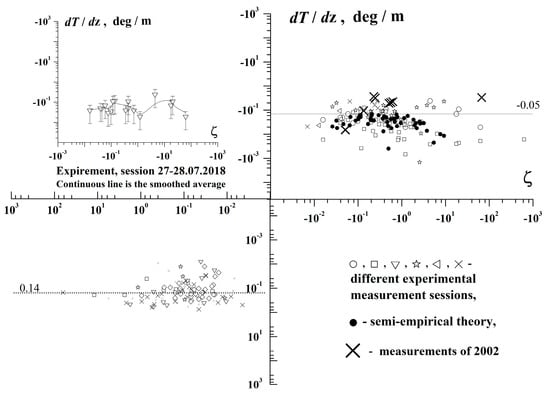
Figure 7.
Comparison experimental (various light symbols for different sessions of measurements) and theoretical values (black circles, the semi-empirical theory) of the vertical derivative of the average air temperature of dT/dz in a mountain boundary layer. Sessions of measurements: ○—27–28.07.18, □—28.07.18, ▽—28.07.18, ☆—28–29.07.18, ◁—29–30.07.18, ×—30.07–01.08.18. In the insert, the measurement session on 27 and 28 July 2018 with confidential intervals for experimental points is shown above on the left. × is the data of measurements from [10,11].
New data of the measurements of spatial derivatives of the temperature of dT/dz in the field of positive, ζ (steady stratification), in which the behavior of derivatives was not investigated earlier (in world scientific literature according to the theory of turbulence for this area, data are absent) are provided in Figure 7. Apparently, in the most part of an interval of positive ζ, the derivative, dT/dz, is close to a constant. This fact can be considered as a new significant result in the similarity theory. Data from Figure 7 allow a more exact form of an asymptotes of universal function of similarity, φ(ζ), to be established at steady stratification (positive values ζ).
As an argument that is applied in Figure 7, one of the main parameters of the MOST is used—the Monin–Obukhov parameter, ζ, and not the commonly used Richardson number, Ri. The Monin–Obukhov parameter, ζ, and the Richardson number, Ri, are related to each other by Equation (24):
where α = Pr −1 is the reverse turbulent Prandtl number.
Ri (z) = ζ/(α φ(ζ)),
As shown in our works (see, for example, [10,11]), the Monin–Obukhov parameter, ζ, can be considered the main turbulence parameter in the anisotropic boundary layer (recently, ζ is often called to as the Monin–Obukhov number by analogy with the Richardson number [10,11]). This parameter changes in the boundary layer when moving from one point to another. It is therefore convenient for describing the turbulent characteristics of an anisotropic boundary layer.
At present, the quantities of α and φ(ζ) can be considered as approximately known for unstable stratification (ζ < 0, more precisely ζ < −0.05). The question of the behavior of the quantities, α and φ(ζ), under stable stratification (ζ > 0, more precisely ζ > +0.05) is still open. For example, the turbulent Prandtl number is not constant under very strong stable stratification, and there are no reliable data on the behavior of the function, φ(ζ), at stable stratification (ζ > +0.05). Therefore, Figure 7 does not contain data for the MOST theory with stable stratification (ζ > 0).
At the same time, as it can be seen from the data of Figure 7, for unstable stratification (ζ < 0), the measurements are consistent with MOST. As can be seen, our measurements are also consistent with MOST in the field of neutral stratification (+0.05 > ζ > −0.05). These are round black dots in Figure 7 to ζ ≈ −0.02 and ζ ≈ −0.03. The applicability of MOST in the field of neutral stratification has received reliable experimental confirmation in the works of other authors. In our opinion, further research is desirable in the field of stable stratification.
4. Conclusions
Thus, a new algorithm for calculating the structural characteristics of temperature fluctuations, as well as the fluctuations of the refractive index and wind speed in the ultrasonic meteorological measuring equipment (anemometers and thermometers) used to study meteorological fields in the surface layer of turbulent atmosphere was constructed. The standard algorithm for calculating the structural characteristics that make sense of the turbulence intensity, usually used in ultrasonic equipment, is based on the Kolmogorov–Obukhov law for structural functions. One of the advantages of ultrasonic systems is their ability to register instantaneous values of the measured characteristics of a turbulent atmosphere with high sampling rates. However, at such high frequencies and at low wind speeds, it is possible to be outside the inertial interval of atmospheric turbulence, where the Kolmogorov–Obukhov law is not applicable, and there is a different behavior of structural functions. This can lead to significant errors in the calculation of the structural characteristics of turbulence. A more advanced algorithm for calculating the parameters proposed in the paper allows more accurate estimation of the structural characteristics of turbulent fluctuations, with an error of not more than 10%.
In the modified ultrasonic complex AMK-03-4 with four ultrasonic anemometers, registration of statistical characteristics of instantaneous spatial derivatives of turbulent fluctuations of temperature and orthogonal components of wind speed, as well as pressure and relative humidity derivatives, were implemented. This makes it possible to study the space–time structure of turbulent meteorological fields of the surface layer of the atmosphere for subsequent applications in the Monin–Obukhov similarity theory and the study of turbulent coherent structures.
For the AMK-03-4 complex, the authors developed an algorithm for determining and eliminating systematic error in the calculation of vertical spatial derivatives of atmospheric parameters from experimental data. This algorithm uses the results of the Monin–Obukhov similarity theory in the field of neutral stratification, for which there is reliable experimental confirmation.
With the use of the complex AMK-03-4, the new data of measurements of the spatial derivatives of temperature in stable stratification (for positive Monin–Obukhov parameters), in which the behavior of the derivatives has not previously been investigated, were obtained. In most of the interval of positive Monin–Obukhov parameters, the vertical derivative of temperature was close to a constant value. This fact can be considered as a new significant result in similarity theory.
Author Contributions
Conceptualization, V.N., V.L., E.N., A.T. and A.B.; Formal analysis, V.N., E.N. and A.T.; Investigation, V.N., E.N. and A.T.; Project administration, V.L.; Resources, V.L.; Software, A.B.; Writing–original draft, A.T.; Writing–review & editing, V.N. and V.L.
Funding
This research was partially funded from the project II.10.3.5 (AAAA-A17–117021310146-3). Analytical generalizations, the algorithms development, the atmospheric turbulence intensity measurements, the error estimations of the ultrasonic meter were partially supported by the Russian Science Foundation (grant No. 17-79-20077).
Conflicts of Interest
The authors declare no conflict of interest.
References
- Gurvich, A.S. Acoustic microanemometer for investigation of the microstructure of turbulence. Acoust. J. 1959, 5, 368–369. [Google Scholar]
- Bovsheverov, V.M.; Voronov, V.P. Acoustic anemometer. Izv. Geophys. Ser. 1960, 6, 882–885. [Google Scholar]
- Mitsuta, Y. Sonic anemometer-thermometer for general use. J. Meteorol. Soc. Jpn. 1966, 44, 12–24. [Google Scholar] [CrossRef][Green Version]
- Mitsuta, Y. Sonic anemometer-thermometer for atmospheric turbulence measurements Flow. Its Measurement and Control in Science and Industry. Instrumen. Soc. Am. 1974, 1, 341–347. [Google Scholar]
- Tikhomirov, A.A. Ultrasonic anemometers and thermometers for measuring fluctuations of air flux velocity and temperature. Review. Opt. Atmos. Okeana 2010, 7, 585–600. Available online: http://ao.iao.ru/en/content/vol.23–2010/iss.07/8 (accessed on 28 May 2019). (In Russian).
- Brock, F.V.; Richardson, S.J. Meteorological Measurement Systems; Oxford University Press: Oxford, UK, 2001; ISBN 9780195134513. [Google Scholar]
- Hanafusa, T.; Fujitani, T.; Kobori, Y.; Mitsuta, Y. A New Type Sonic Anemometer-thermometer for Field Operations. Meteorol. Geophys. 1982, 1, 1–19. [Google Scholar] [CrossRef][Green Version]
- Sozzi, R.; Favaron, M. Sonic anemometry and thermometry: Theoretical basis and data-processing software. Environ. Softw. 1996, 11, 259–270. [Google Scholar] [CrossRef]
- Kaimal, J.C. Sonic Anemometer Measurement of Atmospheric Turbulence. In Proceedings of the Dynamic Flow Conference 1978 on Dynamic Measurements in Unsteady Flows; Springer: Dordrecht, The Netherlands, 1978; pp. 551–565. [Google Scholar]
- Nosov, V.V.; Emaleev, O.N.; Lukin, V.P.; Nosov, E.V. Semiempirical hypotheses of the turbulence theory in anisotropic boundary layer. In Proceedings of the Eleventh International Symposium on Atmospheric and Ocean Optics/Atmospheric Physics, Tomsk, Russian, 15 December 2004; Volume 5743. [Google Scholar]
- Nosov, V.V. Optical Waves and Laser Beams in the Irregular Atmosphere; Blaunshtein, N., Kopeika, N., Eds.; Taylor & Francis Group: Oxfordshire, UK; CRC Press: Boca Raton, FL, USA, 2018; pp. 67–180. [Google Scholar]
- Nosov, V.V.; Grigoriev, V.M.; Kovadlo, P.G.; Lukin, V.P.; Nosov, E.V.; Torgaev, A.V. Turbulent scales of the velocity and temperature in the atmospheric boundary layer. Izv. Vuzov. Fiz. 2013, 8, 331–333. Available online: https://elibrary.ru/item.asp?id=20687071 (accessed on 28 May 2019). (In Russian).
- Monin, A.S.; Yaglom, A.M. Statistical Fluid Mechanics—Vol.1: Mechanics of Turbulence; MIT Press: Cambridge, MA, USA, 1971; Volume 1, ISBN 9780262130622. [Google Scholar]
- Monin, A.S.; Yaglom, A.M. Statistical Fluid Mechanics—Vol.2: Mechanics of Turbulence; MIT Press: Cambridge, MA, USA, 1975; Volume 2, ISBN 9780262130981. [Google Scholar]
- Azbukin, A.A.; Bogushevich, A.Y.; Kobzev, A.A.; Korol’kov, V.A.; Tikhomirov, A.A.; Shelevoi, V.D. AMK-03 Automatic weather stations, their modifications and applications. Datchiki Sist. 2012, 3, 47–52. (In Russian) [Google Scholar]
- Bogushevich, A.Y. Ultrasonic methods for estimation of atmospheric meteorological and turbulence parameters. Atmos. Ocean. Opt. 1999, 2, 164–169. (In Russian) [Google Scholar]
- Bogushevich, A.Y. A software of ultrasonic meteorological stations for investigation of the atmospheric turbulence. Atmos. Ocean. Opt. 1999, 2, 170–174. (In Russian) [Google Scholar]
- Bogushevich, A.Y. Sources of error in ultrasonic measurements of meteorological parameters in the atmosphere, methods and algorithms for minimization on the basis of the experience of creating industrial weather station AMK-03. Fluchen. Zap. Fiz. Fak. Mosk. Univ. 2014, 6, 146308. (In Russian) [Google Scholar]
- Azbukin, A.A.; Bogushevich, A.Y.; Lukin, V.P.; Nosov, V.V.; Nosov, E.V.; Torgaev, A.V. Hardware-Software Complex for Studying the Structure of the Fields of Temperature and Turbulent Wind Fluctuations. Atmos. Ocean. Opt. 2018, 5, 479–485. [Google Scholar] [CrossRef]
- Tatarski, V.I. Wave Propagation in a Turbulent Medium; Dover Publications Inc.: New York, NY, USA, 1961; ISBN 978-0486810294. [Google Scholar]
© 2019 by the authors. Licensee MDPI, Basel, Switzerland. This article is an open access article distributed under the terms and conditions of the Creative Commons Attribution (CC BY) license (http://creativecommons.org/licenses/by/4.0/).